Constant Weight Codes: A Geometric Approach Based on Dissections

Abstract

We present a novel technique for encoding and decoding constant weight binary codes that uses a geometric interpretation of the codebook. Our technique is based on embedding the codebook in a Euclidean space of dimension equal to the weight of the code. The encoder and decoder mappings are then interpreted as a bijection between a certain hyper-rectangle and a polytope in this Euclidean space. An inductive dissection algorithm is developed for constructing such a bijection. We prove that the algorithm is correct and then analyze its complexity. The complexity depends on the weight of the code, rather than on the block length as in other algorithms. This approach is advantageous when the weight is smaller than the square root of the block length.

I Introduction

We consider the problem of encoding and decoding binary codes of constant Hamming weight $w$ and block length $n$. Such codes are useful in a variety of applications: a few examples are fault-tolerant circuit design and computing [15], pattern generation for circuit testing [24], identification coding [26] and optical overlay networks [25].

The problem of interest is that of designing the encoder and decoder, i.e., the problem of mapping all binary (information) vectors of a given length onto a subset of length-$n$ vectors of constant Hamming weight $w$ in a one-to-one manner. In this work, we propose a novel geometric method in which information and code vectors are represented by vectors in $w$-dimensional Euclidean space, covering polytopes for the two sets are identified, and a one-to-one mapping is established by dissecting the covering polytopes in a specific manner. This approach results in an invertible integer-to-integer mapping, thereby ensuring unique decodability. The proposed algorithm has a natural recursive structure, and an inductive proof is given for unique decodability. The issue of efficient encoding and decoding is also addressed. We show that the proposed algorithm has complexity $O(w^{2})$, where $w$ is the weight of the codeword, independent of the codeword length.

Dissections are of considerable interest in geometry, partly as a source of puzzles, but more importantly because they are intrinsic to the notion of volume. Of the $23$ problems posed by David Hilbert at the International Congress of Mathematicians in 1900, the third problem dealt with dissections. Hilbert asked for a proof that there are two tetrahedra of the same volume with the property that it is impossible to dissect one into a finite number of pieces that can be rearranged to give the other, i.e., that the two tetrahedra are not equidecomposable. The problem was immediately solved by Dehn [7]. In 1965, after $20$ years of effort, Sydler [23] completed Dehn’s work. The Dehn-Sydler theorem states that a necessary and sufficient condition for two polyhedra to be equidecomposable is that they have the same volume and the same Dehn invariant. This invariant is a certain function of the edge-lengths and dihedral angles of the polyhedron. An analogous theorem holds in four dimensions (Jessen [11]), but in higher dimensions it is known only that equality of the Dehn invariants is a necessary condition. In two dimensions any two polygons of equal area are equidecomposable, a result due to Bolyai and Gerwein (see Boltianskii [1]). Among other books dealing with the classical dissection problem in two and three dimensions we mention in particular Frederickson [8], Lindgren [13] and Sah [19].

The remainder of the paper is organized as follows. We provide background and review relevant previous work in Section II. Section III describes our geometric approach and gives some low-dimensional examples. Encoding and decoding algorithms are then given in Section IV, and the correctness of the algorithms is established. Section V summarizes the paper.

II Background and Previous Methods

Let us denote the Hamming weight of a length-$n$ binary sequence $\mbox{\boldmath$s$}:=(s_{1},s_{2},\ldots,s_{n})$ by $w(s):=|\{s_{i}:s_{i}=1\}|$, where $|\cdot|$ is the cardinality of a set.

Definition 1

An $(n,w)$ constant weight binary code ${\cal C}$ is a set of length-$n$ sequences such that any sequence $\mbox{\boldmath$s$}\in{\cal C}$ has weight $w(\mbox{\boldmath$s$})=w$.

If $\cal{C}$ is an $(n,w)$ constant weight code, then its rate $R:=(1/n)\log_{2}|{\cal C}|\leq R(n,w):=(1/n)\log_{2}\binom{n}{w}$. For fixed $\beta$ and $w=\left\lfloor\beta n\right\rfloor$, we have

$$\overline{R}:=\lim_{n\rightarrow\infty}R(n,w)=h(\beta)\,,$$ (1)

where $h(\beta):=-\beta\log_{2}(\beta)-(1-\beta)\log_{2}(1-\beta)$ is the entropy function. Thus $\overline{R}$ is maximized when $\beta=1/2$, i.e., the asymptotic rate is highest when the code is balanced.

The (asymptotic) efficiency of a code relative to an infinite-length code with the same weight to length ratio $w/n$, given by $\eta:=R/\overline{R}$, can be written as $\eta=\eta_{1}\overline{\eta}$ where $\eta_{1}:=R/R(n,w)$ and $\overline{\eta}:=R(n,w)/\overline{R}$. The first term, $\eta_{1}$, is the efficiency of a particular code relative to the best possible code with the same length and weight; the second term, $\overline{\eta}$, is the efficiency of the best finite-length code relative to the best infinite-length code.

From Stirling’s formula we have

$$\overline{\eta}\approx 1-\frac{\log_{2}(2\pi n\beta(1-\beta))}{2nh(\beta)}.$$ (2)

A plot of $\overline{\eta}$ as a function of $n$ is given in Fig. 1 for $\beta=1/2$. The slow convergence visible here is the reason one needs codes with large block lengths.

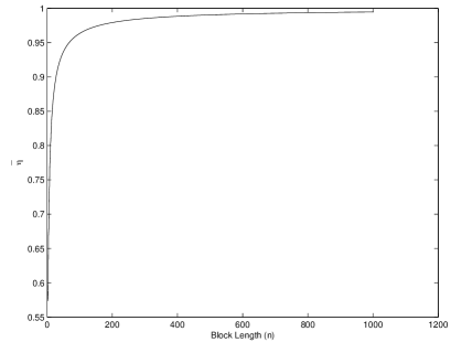
Figure 1: Efficiency $\overline{\eta}$ as a function of block length when $\beta=1/2$

Comprehensive tables and construction techniques for binary constant weight codes can be found in [2] and the references therein. However, the problem of finding efficient encoding and decoding algorithms has received considerably less attention. We briefly discuss two previous methods that are relevant to our work. The first, a general purpose technique based on the idea of lexicographic ordering and enumeration of codewords in a codebook (Schalkwijk [20], Cover [3]) is an example of ranking/unranking algorithms that are well studied in the combinatorial literature (Nijenhuis and Wilf [14]). We refer to this as the enumerative approach. The second (Knuth [12]) is a special-purpose, highly efficient technique that works for balanced codes, i.e., when $w=\lfloor(n/2)\rfloor$, and is referred to as the complementation method.

The enumerative approach orders the codewords lexicographically (with respect to the partial order defined by $0<1$), as in a dictionary. The encoder computes the codeword from its dictionary index, and the decoder computes the dictionary index from the codeword. The method is effective because there is a simple formula involving binomial coefficients for computing the lexicographic index of a codeword. The resulting code is fully efficient in the sense that $\eta_{1}=1$. However, this method requires the computation of the exact values of binomial coefficients $\binom{n}{k}$, and requires registers of length $O(n)$, which limits its usefulness.

An alternative is to use arithmetic coding (Rissanen and Langdon [18], Rissanen [17]; see also Cover and Thomas [4, §13.3]). Arithmetic coding is an efficient variable length source coding technique for finite alphabet sources. Given a source alphabet and a simple probability model for sequences $x$, let $p(\mbox{\boldmath$x$})$ and $F(\mbox{\boldmath$x$})$ denote the probability distribution and cumulative distribution function, respectively. An arithmetic encoder represents $x$ by a number in the interval $(F(\mbox{\boldmath$x$})-p(\mbox{\boldmath$x$}),F(\mbox{\boldmath$x$})]$. The implementation of such a coder can also run into problems with very long registers, but elegant finite-length implementations are known and are widely used (Witten, Neal and Cleary  [28]). For constant weight codes, the idea is to reverse the roles of encoder and decoder, i.e., to use an arithmetic decoder as an encoder and an arithmetic encoder as a constant weight decoder (Ramabadran [16]). Ramabadran gives an efficient algorithm based on an adaptive probability model, in the sense that the probability that the incoming bit is a $1$ depends on the number of $1$’s that have already occurred. This approach successfully overcomes the finite-register-length constraints associated with computing the binomial coefficients and the resulting efficiency is often very high, in many cases the loss of information being at most one bit. The encoding complexity of the method is $O(n)$.

Knuth’s complementation method [12] relies on the key observation that if the bits of a length-$n$ binary sequence are complemented sequentially, starting from the beginning, there must be a point at which the weight is equal to $\lfloor{n/2}\rfloor$. Given the transformed sequence, it is possible to recover the original sequence by specifying how many bits were complemented (or the weight of the original sequence). This information is provided by a (relatively short) constant weight check string, and the resulting code consists of the transformed sequence followed by the constant weight check bits. In a series of papers, Bose and colleagues extended Knuth’s method in various ways, and determined the limits of this approach (see [29] and references therein). The method is simple and efficient, and even though the overall complexity is $O(n)$, for $n=100$ we found it to be eight times as fast as the method based on arithmetic codes. However, the method only works for balanced codes, which restricts its applicability.

The two techniques that we have described above both have complexity that depends on the length $n$ of the codewords. In contrast, the complexity of our algorithm depends only on the weight $w$, which makes it more suitable for codes with relatively low weight.

As a final piece of background information, we define what we mean by a dissection. We assume the reader is familiar with the terminology of polytopes (see for example Coxeter [5], Grünbaum [9], Ziegler [30]). Two polytopes $P$ and $Q$ in $\mathbb{R}^{w}$ are said to be congruent if $Q$ can be obtained from $P$ by a translation, a rotation and possibly a reflection in a hyperplane. Two polytopes $P$ and $Q$ in $\mathbb{R}^{w}$ are said to be equidecomposable if they can be decomposed into finite sets of polytopes $P_{1},\ldots,P_{t}$ and $Q_{1},\ldots,Q_{t}$ , respectively, for some positive integer $t$, such that $P_{i}$ and $Q_{i}$ are congruent for all $i=1,\ldots,t$ (see Frederickson [8]). That is, $P$ is the disjoint union of the polytopes $P_{i}$, and similarly for $Q$. If this is the case then we say that $P$ can be dissected to give $Q$ (and that $Q$ can be dissected to give $P$).

Note that we allow reflections in the dissection: there are at least four reasons for doing so. (i) It makes no difference to the existence of the dissection, since if two polytopes are equidecomposable using reflections they are also equidecomposable without using reflections. This is a classical theorem in two and three dimensions [8, Chap. 20] and the proof is easily generalized to higher dimensions. (ii) When studying congruences, it is simpler not to have to worry about whether the determinant of the orthogonal matrix has determinant $+1$ or $-1$. (iii) Allowing reflections often reduces the number of pieces. (iv) Since our dissections are mostly in dimensions greater than three, the question of “physical realizability” is usually irrelevant. Note also that we do not require that the $P_{i}$ can be obtained from $P$ by a succession of cuts along infinite hyperplanes. All we require is that $P$ be a disjoint union of the $P_{i}$.

One final technical point: when defining dissections using coordinates, as in Eqns. (5), (8) below, we use a mixture of $\leq$ and $<$ signs in order to have unambiguously defined maps. This is essential for our application. On the other hand, it means that the “pieces” in the dissection may be missing certain boundaries. It should therefore be understood that if we were focusing on the dissections themselves, we would replace each piece by its topological closure.

For further information about dissections see the books mentioned in Section I.

III The Geometric Interpretation

In this section, we first consider the problem of encoding and decoding a binary constant weight code of weight $w=2$ and arbitrary length $n$, i.e., where there are only two bits set to $1$ in any codeword. Our approach is based on the fact that vectors of weight two can be represented as points in two-dimensional Euclidean space, and can be scaled, or normalized, to lie in a right triangle. This approach is then extended, first to weight $w=3$, and then to arbitrary weights $w$.

For any weight $w$ and block length $n$, let ${\cal C}_{w}$ denote the set of all weight $w$ vectors, with $|{\cal C}_{w}|=\binom{n}{w}$. Our codebook ${\cal C}$ will be a subset of ${\cal C}_{w}$, and will be equal to ${\cal C}_{w}$ for a fully efficient code, i.e., when $\eta_{1}=1$. We will represent a codeword by the $w$-tuple $\mbox{\boldmath$y^{\prime}$}:=(y^{\prime}_{1},y^{\prime}_{2},\ldots,y^{\prime}_{w})$, $1\leq y^{\prime}_{1}<y^{\prime}_{2}<\ldots<y^{\prime}_{w}\leq n$, where $y^{\prime}_{i}$ is the position of the $i$th $1$ in the codeword, counting from the left. If we normalize these indices $y^{\prime}_{i}$ by dividing them by $n$, the codebook ${\cal C}$ becomes a discrete subset of the polytope $T_{w}$, the convex hull of the points $0^{w},0^{w-1}1,0^{w-2}11,\ldots,01^{w-1},1^{w}$. $T_{2}$ is a right triangle, $T_{3}$ is a right tetrahedron and in general we will call $T_{w}$ a unit orthoscheme.

The set of inputs to the encoder will be denoted by ${\cal R}_{w}$: we assume that this consists of $w$-tuples $\mbox{\boldmath$y$}:=(y_{1},y_{2},\ldots,y_{w})$ which range over a $w$-dimensional hyper-rectangle or “brick”. After normalization by dividing the $y_{i}$ by $n$, we may assume that the input vector is a point in the hyper-rectangle or “brick”

$$B_{w}:=[0,1)\times[1-1/2,1)\times\ldots\times[1-1/w,1)\,.$$

We will use $\mbox{\boldmath$x$}:=(x_{1},x_{2},\ldots,x_{w})=\mbox{\boldmath$y$}/n\in B_{w}$ and $\mbox{\boldmath$x^{\prime}$}:=(x^{\prime}_{1},x^{\prime}_{2},\ldots,x^{\prime}_{w})=\mbox{\boldmath$y^{\prime}$}/n\in T_{w}$ to denote the normalized versions of the input vector and codeword, respectively, defined by $x_{i}:=y_{i}/n$ and $x^{\prime}_{i}:=y^{\prime}_{i}/n$ for $i=1,\ldots,w$.

The basic idea underlying our approach is to find a dissection of $B_{w}$ that gives $T_{w}$. The encoding and decoding algorithms are obtained by tracking how the points $y$ and $y^{\prime}$ move during the dissection.

The volume of $B_{w}$ is $1\times\frac{1}{2}\times\frac{1}{3}\times\cdots\times\frac{1}{w}=\frac{1}{w!}$. This is also the volume of $T_{w}$, as the following argument shows. Classify the points $\mbox{\boldmath$x$}=(x_{1},\ldots,x_{w})$ in the unit cube $[0,1]^{w}$ into $w!$ regions according to their order when sorted; the regions are congruent, so all have volume $1/w!$, and the region where the $x_{i}$ are in nondecreasing order is $T_{w}$.

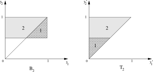
Figure 2: Two ways to dissect rectangle $B_{2}$ to give triangle $T_{2}$. Piece 1 may be rotated about center into its new position, or reflected in main diagonal and translated downwards.

We now return to the case $w=2$. There are many ways to dissect the rectangle $B_{2}$ into the right triangle $T_{2}$. We will consider two such dissections, both two-piece dissections based on Fig. 2.

In the first dissection, the triangular piece marked 1 in Fig. 2 is rotated clockwise about the center of the square until it reaches the position shown on the right in Fig. 2. In the second dissection, the piece marked 1 is first reflected in the main diagonal of the square and then translated downwards until it reaches the position shown on the right in Fig. 2. In both dissections the piece marked 2 is fixed.

The two dissections can be specified in terms of coordinates as follows. For the first dissection, we set

$$\left\{\begin{array}[]{ll}(x^{\prime}_{1},x^{\prime}_{2}):=(x_{1},x_{2})&\mbox{if~{}}x_{1}<x_{2}\\ (x^{\prime}_{1},x^{\prime}_{2}):=(1-x_{1},1-x_{2})&\mbox{if~{}}x_{1}\geq x_{2}\end{array}\right.$$ (5)

and for the second, we set

$$\left\{\begin{array}[]{ll}(x^{\prime}_{1},x^{\prime}_{2}):=(x_{1},x_{2})&\mbox{if~{}}x_{1}<x_{2}\\ (x^{\prime}_{1},x^{\prime}_{2}):=(x_{2}-\frac{1}{2},x_{1}-\frac{1}{2})&\mbox{if~{}}x_{1}\geq x_{2}\end{array}\right.$$ (8)

The first dissection involves only a rotation, but seems harder to generalize to higher dimensions. The second one is the one we will generalize; it uses a reflection, but as mentioned at the end of Section II, this is permitted by the definition of a dissection.

We next illustrate how these dissections can be converted into encoding algorithms for constant weight (weight $2$) binary codes. Again there may be several solutions, and the best algorithm may depend on arithmetic properties of $n$ (such as its parity). We work now with the unnormalized sets ${\cal R}_{2}$ and ${\cal C}_{2}$. In each case the output is a weight-$2$ binary vector with $1$’s in positions $y^{\prime}_{1}$ and $y^{\prime}_{2}$.

III-A First Dissection, Algorithm 1

1. The input is an information vector $(y_{1},y_{2})\in{\cal R}_{2}$ with $1\leq y_{1}\leq n-1$ and $\lceil n/2\rceil+1\leq y_{2}\leq n$.

2. If $y_{1}<y_{2}$, we set $y^{\prime}_{1}=y_{1}$, $y^{\prime}_{2}=y_{2}$, otherwise we set $y^{\prime}_{1}=n-y_{1}$ and $y^{\prime}_{2}=n-y_{2}+1$.

For $n$ even, this algorithm generates all possible $n(n-1)/2$ codewords. For $n$ odd it generates only $(n-1)^{2}/2$ codewords, leading to a slight inefficiency, and the following algorithm is to be preferred.

III-B First Dissection, Algorithm 2

1. The input is an information vector $(y_{1},y_{2})\in{\cal R}_{2}$ with $1\leq y_{1}\leq n$, $\lceil(n+1)/2\rceil+1\leq y_{2}\leq n$.

2. If $y_{1}<y_{2}$, we set $y^{\prime}_{1}=y_{1}$, $y^{\prime}_{2}=y_{2}$, otherwise we set $y^{\prime}_{1}=n-y_{1}+1$, $y^{\prime}_{2}=n-y_{2}+2$.

For $n$ odd, this algorithm generates all $n(n-1)/2$ codewords, but for $n$ even it generates only $n(n-1)/2$ codewords, again leading to a slight inefficiency.

III-C Second Dissection

1. The input is an information vector $(y_{1},y_{2})\in{\cal R}_{2}$ with $1\leq y_{1}\leq n-1$ and $\lceil n/2\rceil+1\leq y_{2}\leq n$.

2. If $y_{1}<y_{2}$, we set $y^{\prime}_{1}=y_{1}$, $y^{\prime}_{2}=y_{2}$, otherwise we set $y^{\prime}_{1}=y_{2}-\lceil n/2\rceil$, $y^{\prime}_{2}=y_{1}-\lceil n/2\rceil+1$.

For $n$ even, this algorithm generates all $n(n-1)/2$ codewords, but for $n$ odd it generates only $(n-1)^{2}/2$ codewords, leading to a slight inefficiency. There is a similar algorithm, not given here, which is better when $n$ is odd.

Note that only one test is required in any of the encoding algorithms. The mappings are invertible, with obvious decoding algorithms corresponding to the inverse mappings from ${\cal C}_{2}$ to ${\cal R}_{2}$

We now extend this method to weight $w=3$. Fortunately, the Dehn invariants for both the brick $B_{3}$ and our unit orthoscheme $T_{3}$, which is the tetrahedron with vertices $(0,0,0),(0,0,1),(0,1,1)$ and $(1,1,1)$, are zero (since in both cases all dihedral angles are rational multiples of $\pi$), and so by the Dehn-Sydler theorem the polyhedra $B_{3}$ and $T_{3}$ are equidecomposable. As already mentioned in Section I, the Dehn-Sydler theorem applies only in three dimensions. But it will follow from the algorithm given in the next section that $B_{w}$ and $T_{w}$ are equidecomposable in all dimensions.

We will continue to describe the encoding step (the map from $B_{w}$ to $T_{w}$) first. We will give an inductive dissection (see Fig. 3), transforming $B_{3}$ to $T_{3}$ in two steps, effectively reducing the dimension by one at each step. In the first step, the brick $B_{3}$ is dissected into a triangular prism (the product of a right triangle, $T_{2}$, and an interval), and in the second step this triangular prism is dissected into the tetrahedron $T_{3}$. Note that the first step has essentially been solved by the dissection given in Eqn. (8).

Figure 3: Transformation from tetrahedron to rectangular prism.

For the second step we use a four-piece dissection of the triangular prism to the tetrahedron $T_{3}$. This dissection, shown with the tetrahedron and prism superimposed in Fig. 4, appears to be new.

There is a well-known dissection of the same pair of polyhedra that was first published by Hill in 1896 [10]. This also uses four pieces, and is discussed in several references: see Boltianskii [1, p. 99], Cromwell [6, p. 47], Frederickson [8, Fig. 20.4], Sydler [22], Wells [27, p. 251]. However, Hill’s dissection seems harder to generalize to higher dimensions. Hill’s dissection does have the advantage over ours that it can be accomplished purely by translations and rotations, whereas in our dissection two of the pieces (pieces labeled 2 and 3 in Fig. 4) are also reflected. However, as mentioned at the end of Section II, this is permitted by the definition of a dissection, and is not a drawback for our application. Apart from this, our dissection is simpler than Hill’s, in the sense that his dissection requires a cut along a skew plane ($x_{1}-x_{3}=1/3$), whereas all our cuts are parallel to coordinate axes.

Figure 4: Four-piece dissection of tetrahedron to triangular prism. Pieces 2 and 3 are reflected.

To obtain the four pieces shown in Fig. 4, we first make two horizontal cuts along the planes $x_{3}=\frac{1}{3}$ and $x_{3}=\frac{2}{3}$, dividing the tetrahedron into three slices. We then cut the middle slice into two by a vertical cut along the plane $x_{2}=\frac{1}{2}$.

There appears to be a tradition in geometry books that discuss dissections of not giving coordinates for the pieces. To an engineer this seems unsatisfactory, and so in Table I we list the vertices of the four pieces in our dissection. Piece 1 has four vertices, while the other three pieces each have six vertices. (In the Hill dissection the numbers of vertices of the four pieces are $4$, $5$, $6$ and $6$ respectively.) Given these coordinates, it is not difficult to verify that the four pieces can be reassembled to form the triangular prism, as indicated in Fig. 4. As already remarked, pieces 2 and 3 are also reflected (or “turned over” in a fourth dimension). The correctness of the dissection also follows from the alternative description of this dissection given below.

$$\begin{array}[]{|c|l|}\hline\cr\mbox{Piece}&\mbox{Coordinates}\\ \hline\cr 1&[0,0,0],[0,0,1/3],[0,1/3,1/3],[1/3,1/3,1/3].\\ 2&[0,0,1/3],[0,1/3,1/3],[1/3,1/3,1/3],\\ &[0,0,2/3],[0,1/3,2/3],[1/3,1/3,2/3].\\ 3&[0,1/3,1/3],[1/3,1/3,1/3],[0,1/3,2/3],\\ &[0,2/3,2/3],[2/3,2/3,2/3],[1/3,1/3,2/3].\\ 4&[0,0,2/3],[0,2/3,2/3],[2/3,2/3,2/3],\\ &[0,0,1],[0,1,1],[1,1,1].\\ \hline\cr\end{array}$$

TABLE I: Coordinates of vertices of pieces in dissection of tetrahedron shown in Fig. 4.

The dissection shown in Fig. 4 can be described algebraically as follows. We describe it in the more logical direction, going from the triangular prism to the tetrahedron since this is what we will generalize to higher dimensions in the next section. The input is a vector $(x_{1},x_{2},x_{3})$ with $0\leq x_{1}\leq x_{2}<1$, $\frac{2}{3}\leq x_{3}<1$; the output is a vector $(x^{\prime}_{1},x^{\prime}_{2},x^{\prime}_{3})$ with $0\leq x^{\prime}_{1}\leq x^{\prime}_{2}\leq x^{\prime}_{3}<1$, given by $(x^{\prime}_{1},x^{\prime}_{2},x^{\prime}_{3})=$

$$\left\{\begin{array}[]{ll}(x_{1},x_{2},x_{3})&\mbox{if~{}}x_{1}\leq x_{2}<x_{3}\\ (x_{1}-\frac{1}{3},x_{3}-\frac{1}{3},x_{2}-\frac{1}{3})&\mbox{if~{}}\frac{1}{3}\leq x_{1}<x_{3}\leq x_{2}\\ (x_{3}-\frac{2}{3},x_{2}-\frac{2}{3},x_{1}+\frac{1}{3})&\mbox{if~{}}x_{1}\leq\frac{1}{3}<x_{3}\leq x_{2}\\ (x_{3}-\frac{2}{3},x_{1}-\frac{2}{3},x_{2}-\frac{2}{3})&\mbox{if~{}}x_{3}\leq x_{1}\leq x_{2}\end{array}\right.$$ (13)

The four cases in Eqn. (13), after being transformed, correspond to the pieces labeled 4, 3, 2, 1 respectively in Fig. 4. We see from Eqn. (13) that in the second and third cases the linear transformation has determinant $-1$, indicating that these two pieces must be reflected.

Since it is hard to visualize dissections in dimensions greater than three, we give a schematic representation of the above dissection that avoids drawing polyhedra. Fig. 5 shows a representation of the transformation from the triangular prism to the tetrahedron $T_{3}$, equivalent to that given in Eqn. (13). The steps shown in Fig. 5 may be referred to as “cut and paste” operations, because, as Fig. 5 shows, the vector in the triangular prism is literally cut up into pieces which are rearranged and relabeled. Note that, to complete the transformation, we precede this operation by the dissection given in Eqn. (8), finally establishing the bijection between $B_{3}$ and $T_{3}$.

Figure 5: Cut-and-paste description of the inverse transformation from triangular prism to tetrahedron.

We now describe the mapping shown in Fig. 5 in more detail. The triangular prism is represented by the set of partially ordered triples $(x_{1},x_{2},x_{3})$ with $0\leq x_{1}\leq x_{2}<1$ and $\frac{2}{3}\leq x_{3}<1$, and we wish to transform this into the tetrahedron consisting of the points $(x^{\prime}_{1},x^{\prime}_{2},x^{\prime}_{3})$ with $0\leq x^{\prime}_{1}\leq x^{\prime}_{2}\leq x^{\prime}_{3}<1$.

We divide the interval $[0,1)$ into $w=3$ equal segments of length $1/w=1/3$, and consider where the points $x_{1},x_{2}$ and $x_{3}$ fall in this interval, given that $(x_{1},x_{2},x_{3})$ is in the triangular prism. There are three possibilities for where $x_{3}$ lies in relation to $0\leq x_{1}\leq x_{2}<1$, and we further divide the case $x_{1}\leq x_{3}<x_{2}$ into two subcases depending on whether $x_{1}\geq\frac{1}{3}$ or $x_{1}<\frac{1}{3}$. These are the four cases shown in Fig. 5, and correspond one-to-one with the four dissection pieces in Fig. 4. Fig. 5 shows how the triples $x_{1},x_{2},x_{3}$ (reindexed according to their relative positions) are mapped to the triples $x^{\prime}_{1},x^{\prime}_{2},x^{\prime}_{3}$.

The last column of Fig. 5 shows the ranges of the $x^{\prime}_{i}$ in the four cases; the fact that these ranges are disjoint guarantees that the mapping from $x_{1},x_{2},x_{3}$ to $x^{\prime}_{1},x^{\prime}_{2},x^{\prime}_{3}$ is invertible. The ranges of the $x^{\prime}_{i}$ will be discussed in more detail in the following section after the general algorithms are presented.

This operation can now be described without explicitly mentioning the underlying dissection. Each interval of length $1/w$, together with the given $x_{i}$ values within it, is treated as a single complete unit. In the “cut and paste” operations, these units are rearranged and relabeled in such a way that the operation is invertible.

IV Algorithms and Proof of Correctness

In the previous section we provided an encoding and decoding algorithm for weights $w=2$ and $w=3$, based on our geometric interpretation of ${\cal C}_{2}$ and ${\cal C}_{3}$ as points in $\mathbb{R}^{w}$. In this section, the algorithm is generalized to larger values of the weight $w$. We start with the geometry, and give a dissection of the “brick” $B_{w}$ into the orthoscheme $T_{w}$. We work with the normalized coordinates $x_{i}=y_{i}/n$ (for a point in $B_{w}$) and $x^{\prime}_{i}=y^{\prime}_{i}/n$ (for a point in $T_{w}$), where $1\leq i\leq w$. Later in this section, we discuss the modifications needed to take into account the fact that the $y^{\prime}_{i}$ must be integers.

IV-A An Inductive Decomposition of the Orthoscheme

Restating the problem, we wish to find a bijection $F_{w}$ between the sets $B_{w}$ and $T_{w}$. The inductive approach developed for $w=3$ (where the $w=2$ case was a subproblem) will be generalized. Of course the bijection $F_{1}$ between $B_{1}$ and $T_{1}$ is trivial. We assume that a bijection $F_{w-1}$ is known between $B_{w-1}$ and $T_{w-1}$, and show how to construct a bijection $F_{w}$ between $B_{w}$ and $T_{w}$.

The last step in the induction uses a map $f_{w}$ from the prism $T_{w-1}\times[1-\frac{1}{w},1)$ to ${T_{w}}$ ($f_{2}$ is the map described in Eqn. (8) and $f_{3}$ is described in Eqn. (13)). The mapping $F_{w}$ from $B_{w}$ to $T_{w}$ is then given recursively by $F_{w}:(x_{1},x_{2},\ldots,x_{w})\mapsto(x^{\prime}_{1},x^{\prime}_{2},\ldots,x^{\prime}_{w})$, where

$$(x^{\prime}_{1},x^{\prime}_{2},\ldots,x^{\prime}_{w}):=f_{w}(F_{w-1}(x_{1},x_{2},\ldots,x_{w-1}),x_{w})\,.$$ (14)

For $w=1$ we set

$$F_{1}:=f_{1}:B_{1}\rightarrow T_{1},~{}(x_{1})\mapsto(x^{\prime}_{1})=(x_{1})\,.$$

By iterating Eqn. (14), we see that $F_{w}$ is obtained by successively applying the maps $f_{1},f_{2},$…, $f_{w}$.

The following algorithm defines $f_{w}$ for $w\geq 2$. We begin with an algebraic definition of the mapping and its inverse, and then discuss it further in the following section. The input to the mapping $f_{w}$ is a vector $\mbox{\boldmath$x$}:=(x_{1},x_{2},\ldots,x_{w})$, with $(x_{1},x_{2},\ldots,x_{w-1})\in T_{w-1}$ and $x_{w}\in[1-1/w,1)$; the output is a vector $\mbox{\boldmath$x^{\prime}$}:=(x^{\prime}_{1},x^{\prime}_{2},\ldots,x^{\prime}_{w})\in T_{w}$.

Forward mapping $f_{w}$ ($w\geq 2$):

1) Let

$$i_{0} := \min\{i\in\{1,\ldots,w\}\mid x_{w}\leq x_{i}\}\,.$$

2) Let

$$j_{0} := \min\{i\in\{1,\ldots,i_{0}\}\mid w-i_{0}+i-1\leq wx_{i}\}-1\,.$$

3) Set $x_{k}^{\prime}$ equal to:

$$\left\{\begin{array}[]{ll}x_{k+j_{0}}-\frac{w+j_{0}-i_{0}}{w}&\mbox{for~{}}k=1,\ldots,i_{0}-j_{0}-1\\ x_{w}-\frac{w+j_{0}-i_{0}}{w}&\mbox{for~{}}k=i_{0}-j_{0}\\ x_{k+j_{0}-1}-\frac{w+j_{0}-i_{0}}{w}&\mbox{for~{}}k=i_{0}-j_{0}+1,\ldots,w-j_{0}\\ x_{k-w+j_{0}}+\frac{i_{0}-j_{0}}{w}&\mbox{for~{}}k=w-j_{0}+1,\ldots,w\end{array}\right.$$ (19)

Eqn. (19) identifies the “cut and paste” operations required to obtain $x^{\prime}_{k}$ for different ranges of the variable $k$. If the initial index in one of the four cases in Eqn. (19) is smaller than the final index, that case is to be skipped. A case is also skipped if the subscript for an $x_{i}$ is not in the range $1,\ldots,w$. Note in Step 1 that $i_{0}=w$ if $x_{w}$ is the largest of the $x_{i}$’s. This implies that $j_{0}=0$, and then Step 3 is the identity map.

The inverse mapping $G_{w}$ from $T_{w}$ to $B_{w}$ has a similar recursive definition. The $w$th step in the induction is the map $g_{w}:T_{w}\rightarrow{T_{w-1}\times[1-\frac{1}{w},1)}$ defined below. For $w=1$ we set

$$G_{1}:=g_{1}:T_{1}\rightarrow B_{1},(x^{\prime}_{1})\mapsto(x_{1})=(x^{\prime}_{1})\,.$$

The map $G_{w}$ is obtained by successively applying the maps $g_{w},g_{w-1},$…, $g_{1}$.

Inverse mapping $g_{w}$ ($w\geq 2$):

1) Let

$$m_{0} := \max\{i\in\{1,\ldots,w\}\mid i-1\leq wx^{\prime}_{i}\}\,.$$

2) If $m_{0}=w$, let $j_{0}:=0$, otherwise let

$$j_{0} := w-\max\{i\in\{m_{0}+1,\ldots,w\}\mid wx^{\prime}_{i}\leq m_{0}\}\,;$$

in either case, let $i_{0}:=j_{0}+m_{0}$.

3) Set $x_{k}$ equal to:

$$\left\{\begin{array}[]{ll}x_{k+w-j_{0}}^{\prime}-\frac{i_{0}-j_{0}}{w}&\mbox{for~{}}k=1,\ldots,j_{0}\\ x_{k-j_{0}}^{\prime}+\frac{w+j_{0}-i_{0}}{w}&\mbox{for~{}}k=j_{0}+1,\ldots,i_{0}-1\\ x_{k-j_{0}+1}^{\prime}+\frac{w+j_{0}-i_{0}}{w}&\mbox{for~{}}k=i_{0},\ldots,w-1\\ x_{i_{0}-j_{0}}^{\prime}+\frac{w+j_{0}-i_{0}}{w}&\mbox{for~{}}k=w\end{array}\right.$$ (24)

Note that the transformations in Eqn. (19) and Eqn. (24) are formal inverses of each other, and that these transformations are volume-preserving. The underlying linear transformations are orthogonal transformations with determinant $+1$ or $-1$.

Before proceeding further, let us verify that in the case $w=3$, the mapping $f_{w}=f_{3}$ agrees with that given in Eqn. (13).

• If $x_{1}\leq x_{2}<x_{3}$, then $i_{0}=3$, $j_{0}=0$ and the map is the identity, as mentioned above.

• If $x_{1}<x_{3}\leq x_{2}$ there are two subcases:

  • If $\frac{1}{3}\leq x_{1}$ then $i_{0}=2$, $j_{0}=0$.

  • If $x_{1}<\frac{1}{3}$ then $i_{0}=2$, $j_{0}=1$.

• If $x_{3}\leq x_{1}\leq x_{2}$, then $i_{0}=1$, $j_{0}=0$.

The transformations in Eqn. (19) now exactly match those in Eqn. (13).

IV-B Interpretations and Explanations

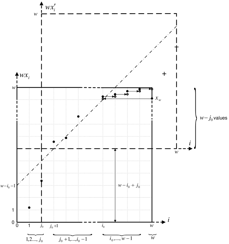
Figure 6: A graphical illustration of the forward and inverse mapping.

In Fig. 6, we give a graphical interpretation of the algorithm, which can be regarded as a generalization of the “cut and paste” description given above. This figure shows the transformation defined by the $w$th step $f_{w}$ in the algorithm. At this step, we begin with a list of $w-1$ numbers $(x_{1},x_{2},\ldots,x_{w-1})$ in increasing order, and a further number $x_{w}$ which may be anywhere in the interval $[1-1/w,1)$. This list of $w$ numbers is plotted in the plane as the set of $w$ points $(i,wx_{i})$ for $i=1,2,\ldots,w$ (indicated by the solid black circles in Fig. 6). In the first step in the forward algorithm, the augmented list $(x_{1},x_{2},\ldots,x_{w})$ is sorted into increasing order. In the sorted list, $x_{w}$ now occupies position ${i_{0}}$, so the point $(w,wx_{w})$ moves to the left, to the new position $(i_{0},wx_{w})$, and the points $(i,wx_{i})$ for $i=i_{0}+1,\ldots,w-1$ move to the right. This is indicated by the arrows in the figure. The new positions of these points are marked by hollow circles.

The point $(i_{0},wx_{w})$ now lies between the grid points $(i_{0},w)$ and $(i_{0},w-1)$ (it may coincide with the latter point), since $x_{w}\geq 1-\frac{1}{w}$. We draw the line $y=x+w-i_{0}-1$ (shown as the dashed-and-dotted line in Fig. 6). This has unit slope and passes through the points $(i_{0},w-1)$ and $(0,w-i_{0}-1)$. The algorithm then computes $j_{0}+1$ to be the smallest index $i$ for which $x_{i}$ is on or above this line. Once $i_{0}$ and $j_{0}$ have been determined, the forward mapping proceeds as follows. The points $(i,wx_{i})$ for $i=1,\ldots,j_{0}$ are shifted to the right of the figure and are moved upwards by the amount $(i_{0}-j_{0})/w$, their new positions being indicated by crosses in the figure. Finally, the origin is moved to the grid point $(j_{0},w-i_{0}+j_{0})$ and the points are reindexed. The $m_{0}:=i_{0}-j_{0}$ points which originally had indices $j_{0}+1,\ldots,i_{0}$ become points $1,\ldots,m_{0}$ after reindexing. In the new coordinates, the final positions of the points lie inside the square region $[1,w)\times[1,w)$. The reader can check that this process is exactly equivalent to the algebraic description of $f_{w}$ given above.

To recover $i_{0}$ and $j_{0}$, we first determine the value of $m_{0}:=i_{0}-j_{0}$. This can indeed be done since $m_{0}$ is precisely the index of the largest $wx^{\prime}_{i}$ that lies on or above the line $y=x-1$ in the new coordinate system. Note that the position of this line is independent of $i_{0}$ and $j_{0}$ and $(x^{\prime}_{1},x^{\prime}_{2},\ldots,x^{\prime}_{w})$. This works because the points $wx_{1},\ldots,wx_{j_{0}}$ in the original coordinate system, before the origin is shifted, are moved right by $w$ units and upwards by $w$ units, so points below the dashed-and-dotted line remain below the line. Furthermore, observe that in the new coordinate system the number of points $(i,wx^{\prime}_{i})$ below the line $y=m_{0}$ is equal to $w-j_{0}$. Thus the correct $i_{0}$ and $j_{0}$ values may be recovered, and the inverse mapping can be successfully performed.

The following remarks record two properties of the algorithm that will be used later.

Remark 1: Step 2 of the forward algorithm implies that $x_{j_{0}}<\frac{w-i_{0}+j_{0}-1}{w}$ and $x_{j_{0}+1}\geq{\frac{w-i_{0}+j_{0}}{w}}$. It follows that there is no $i$ in the range $1\leq{i}\leq{w}$ for which

$$\frac{w-i_{0}+j_{0}-1}{w}\leq{x_{i}}<\frac{w-i_{0}+j_{0}}{w}\,.$$

Remark 2: The forward algorithm produces a vector $x^{\prime}$ whose components satisfy

$$0\leq{x_{1}^{\prime}}\leq\cdots\leq{x_{i_{0}-j_{0}}^{\prime}}\leq\cdots\leq{x_{w-j_{0}}^{\prime}}<\frac{i_{0}-j_{0}}{w}\,,$$ (25)

$$\frac{i_{0}-j_{0}}{w}\leq{x_{w-j_{0}+1}^{\prime}}\leq{x_{w-j_{0}+2}^{\prime}}\leq\cdots\leq{x_{w}^{\prime}}<1\,,$$ (26)

and

$${x_{k}^{\prime}}<\frac{k-1}{w},\mbox{~{}for~{}}w-j_{0}+1\leq{k}\leq{w}\,.$$ (27)

Eqns. (25) and (26) follow from the minimizations in Steps 1 and 2 of the forward algorithm, respectively. The right-hand side of Eqn. (27) expresses the fact, already mentioned, that the first $j_{0}$ points remain below the dotted-and-dashed line after they are shifted.

IV-C Proof of Correctness

We now give the formal proof that the algorithm is correct. This is simply a matter of collecting together facts that we have already observed.

Theorem 1

For any $w\geq 1$, the forward mapping $f_{w}$ is a one-to-one mapping from ${T_{w-1}\times{[1-\frac{1}{w},1)}}$ to $T_{w}$ with inverse $g_{w}$.

Proof: First, it follows from Remark 2 that, for $\mbox{\boldmath$x$}\in{T_{w-1}\times{[1-\frac{1}{w},1)}}$, $\mbox{\boldmath$x^{\prime}$}=(x_{1}^{\prime},x_{2}^{\prime},\ldots,x_{w}^{\prime})$ satisfies $0\leq{x_{1}^{\prime}}\leq{x_{2}^{\prime}}\leq\cdots\leq{x_{w}^{\prime}}<1$, and so is an element of $T_{w}$.

Suppose there were two different choices for $x$, say $\mbox{\boldmath$x$}^{(1)}$ and $\mbox{\boldmath$x$}^{(2)}$, such that

$$f_{w}(\mbox{\boldmath$x$}^{(1)})=f_{w}(\mbox{\boldmath$x$}^{(2)})=\mbox{\boldmath$x$}^{\prime}\,.$$

We know that $\mbox{\boldmath$x$}^{\prime}$ determines $m_{0},j_{0}$ and $i_{0}$. So $\mbox{\boldmath$x$}^{(1)}$ and $\mbox{\boldmath$x$}^{(2)}$ have the same associated values of $i_{0}$ and $j_{0}$. But for a given pair $(i_{0},j_{0})$, Eqn. (19) is invertible. Hence $\mbox{\boldmath$x$}^{(1)}=\mbox{\boldmath$x$}^{(2)}$, and $f_{w}$ is one-to-one.

Note that the transformations in Eqn. (19) and Eqn. (24) are inverses of each other. Hence $f_{w}$ is also an onto map, and $g_{w}$ is its inverse.  

IV-D Number of Pieces

The map $f_{w}$, which dissects the prism $T_{w-1}\times[1-\frac{1}{w},1)$ to give the orthoscheme ${T_{w}}$, has one piece for each pair $(i_{0},j_{0})$. If $i_{0}=w$ then $j_{0}=0$, while if $1\leq i_{0}\leq w-1$, $j_{0}$ takes all values from $0$ to $i_{0}-1$. (It is easy to write down an explicit point in the interior of the piece corresponding to a specified pair of values of $i_{0}$ and $j_{0}$. Assume $i_{0}<w$ and set $\delta=1/w^{3}$. Take the point with coordinates $(x_{1},\ldots,x_{w})$ given by $x_{w}=(w-1)/w+\delta$; $x_{i}=x_{w}+\delta(i-i_{0})$ for $i=i_{0}+1,\ldots,w-1$; $x_{i}=(i+w-i_{0}-1-\delta)/w$ for $i=1,\ldots,j_{0}$; $x_{i}=(i+w-i_{0}-1+\delta)/w$ for $i=j_{0}+1,\ldots,i_{0}-1$.) The total number of pieces in the dissection is therefore

$$1+1+2+3+\cdots+(w-1)=\frac{w^{2}-w+2}{2}\,,$$

which is $1,2,4,7,11,\ldots$ for $w=1,2,3,4,5,\ldots$. This is a well-known sequence, entry A124 in [21], which by coincidence also arises in a different dissection problem: it is the maximal number of pieces into which a circular disk can be cut with $w-1$ straight cuts. For example, with three cuts, a pizza can be cut into a maximum of seven pieces, and this is also the number of pieces in the dissection defined by $f_{4}$.

IV-E The Algorithms for Positive Integers

To apply the above algorithm to the problem of encoding and decoding constant weight codes, we must work with positive integers rather than real numbers, which entails a certain loss in rate, although the algorithms remain largely unchanged. Let $\mathbb{N}:=\{1,2,3,\ldots\}$, and let $n$ and $w$ be given with $2w<n$. In a manner analogous to the real-valued case, we find a bijection between a finite hyper-rectangle or brick $B_{w}^{\mathbb{N}}\subset{{\mathbb{N}}^{w}}$ and a subset of the finite orthoscheme $T_{w}^{\mathbb{N}}\subset{{\mathbb{N}}^{w}}$, where $B_{w}^{\mathbb{N}}$ is the set of vectors $(y_{1},y_{2},\ldots,y_{w})\in{{\mathbb{N}}^{w}}$ satisfying

$$n-(w-i)-\lfloor{\frac{n-(w-i)}{i}}\rfloor+1\leq{y_{i}}\leq{n-(w-i)}\,,$$

for $i=1,2,\ldots,w$, and $T_{w}^{\mathbb{N}}$ is the set of vectors $(y_{1},y_{2},\ldots,y_{w})\in{{\mathbb{N}}^{w}}$ satisfying

$$1\leq{y_{1}}<y_{2}<\cdots<y_{w}\leq{n}\,.$$

Note that usually $|B_{w}^{\mathbb{N}}|<|T_{w}^{\mathbb{N}}|$, which entails a loss in rate.

The forward mapping $f_{w}$ is now replaced by the map $f^{\mathbb{N}}_{w}$, which sends $(y_{1},y_{2},\ldots,y_{w})$ with $(y_{1},y_{2},\ldots,y_{w-1})\in{T_{w-1}^{\mathbb{N}}}$ and ${n-\lfloor\frac{n}{w}\rfloor+1}\leq{y_{w}}\leq{n}$ to an element of ${T_{w}^{\mathbb{N}}}$. Let us write $n=pw+q$, where $p\geq{0}$ and $0\leq{q}\leq{w-1}$. We partition the range $1,2,\ldots,n$ into $w$ parts, where the first $n-w-1$ parts each have $p$ elements, the next $q$ parts each have $p+1$ elements, and the last part has $p$ elements (giving a total of $n$ elements). This is similar to the real-valued case, where each interval had length $1/w$.

1) Let

$$i_{0} := \min\{i\in\{1,\ldots,w\}\mid y_{w}\leq y_{i}\}\,.$$

2) Let

$$j_{0} := \min\{i\in\{1,\ldots,i_{0}\}\mid V_{i}<y_{i}\}-1\,,$$

where $V_{i}:=(w-i_{0}+i-1)p+\max\{q-i_{0}+i,0\}$.

3) Set $y_{k}^{\prime}$ equal to:

$$\left\{\begin{array}[]{ll}y_{k+j_{0}}-V_{j_{0}+1}&\mbox{for~{}}k=1,\ldots,i_{0}-j_{0}-1\\ y_{w}-V_{j_{0}+1}&\mbox{for~{}}k=i_{0}-j_{0}\\ y_{k+j_{0}-1}+1-V_{j_{0}+1}&\mbox{for~{}}k=i_{0}-j_{0}+1,\ldots,w-j_{0}\\ y_{k-w+j_{0}}+n-V_{j_{0}+1}&\mbox{for~{}}k=w-j_{0}+1,\ldots,w\end{array}\right.$$ (32)

The inverse mapping $g_{w}$ is similarly replaced by the map $g^{\mathbb{N}}_{w}:{T_{w}^{\mathbb{N}}}\rightarrow\{(y_{1},y_{2},\ldots,y_{w}):(y_{1},y_{2},\ldots,y_{w-1})\in{T_{w-1}^{\mathbb{N}}},$ ${n-\lfloor\frac{n}{w}\rfloor+1}\leq{y_{w}}\leq{n}\}$, defined as follows. Again, assume $n=pw+q$.

1) Let

$$m_{0} := \max\{i\in\{1,\ldots,w\}\mid W_{i}<y^{\prime}_{i}\}\,,$$

where $W_{i}:=q+(i-1)p+\min\{i-q-1,0\}$.

2) If $m_{0}=w$, let $j_{0}:=0$, otherwise let

$$j_{0} := w-\max\{i\in\{m_{0}+1,\ldots,w\}\mid y^{\prime}_{i}\leq W_{m_{0}}+p\}\,;$$

in either case, let $i_{0}:=j_{0}+m_{0}$.

3) Set $y_{k}$ equal to:

$$\left\{\begin{array}[]{ll}y_{k+w-j_{0}}^{\prime}-p-W_{m_{0}}&\mbox{for~{}}k=1,\ldots,j_{0}\\ y_{k-j_{0}}^{\prime}+n-p-W_{m_{0}}&\mbox{for~{}}k=j_{0}+1,\ldots,i_{0}-1\\ y_{k-j_{0}+1}^{\prime}-1+n-p-W_{m_{0}}&\mbox{for~{}}k=i_{0},\ldots,w-1\\ y_{i_{0}-j_{0}}^{\prime}+n-p-W_{m_{0}}&\mbox{for~{}}k=w\end{array}\right.$$ (37)

We omit the proofs, since they are similar to those for the real-valued case.

IV-F Comments on the Algorithm

The overall complexity of the transform algorithm is $O(w^{2})$, because at each induction step the complexity is linear in the weight at that step. Recall that the complexities of the arithmetic coding method and Knuth’s complementation method are both $O(n)$. Thus when the weight $w$ is larger than $\sqrt{n}$, the geometric approach is less competitive. When the weight is low, the proposed geometric technique is more efficient, because Knuth’s complementation method is not applicable, while the dissection operations of the proposed algorithm makes it faster than the arithmetic coding method. Furthermore, due to the structure of the algorithm, it is possible to parallelize part of the computation within each induction step to further reduce the computation time.

So far little has been said about mapping a binary sequence to an integer sequence $y_{1},y_{2},\ldots,y_{w}$ such that $y_{i}\in[L_{i},U_{i}]$, where $L_{i}$ and $U_{i}$ are the lower and upper bound of the valid range as specified by the algorithm. A straightforward method is to treat the binary sequence as an integer number and then use “quotient and remainder” method to find such a mapping. However, this requires a division operation, and when the binary sequence is long, the computation is not very efficient. A simplification is to partition the binary sequence into short sequences, and map each short binary sequence to a pair of integers, as in the case of a weight two constant weight codes. Through proper pairing of the ranges, the loss in the rate can be minimized.

The overall rate loss has two components, the first from the rounding involved in using natural numbers, the second from the loss in the above simplified translation step. However, when the weight is on the order of $\sqrt{n}$, and $n$ is in the range of $100-1000$, the rate loss is usually $1-3$ bits per block. For example, when $n=529$, $w=23$, then the rate loss is 2 bits/block compared to the best possible code which would encode $k_{0}=132$ information bits.

V Conclusion

We propose a novel algorithm for encoding and decoding constant weight binary codes, based on dissecting the polytope defined by the set of all binary words of length $n$ and weight $w$, and reassembling the pieces to form a hyper-rectangle corresponding to the input data. The algorithm has a natural recursive structure, which enables us to give an inductive proof of its correctness. The proposed algorithm has complexity $O(w^{2})$, independent of the length of the codewords $n$. It is especially suitable for constant weight codes of low weight.

References

- [1] V. G. Boltianskii, Hilbert’s Third Problem, Translated from the Russian by R. A. Silverman, Wiley, NY, 1978.
- [2] A. E. Brouwer, J. B. Shearer, N. J. A. Sloane and W. D. Smith, “A new table of constant weight codes,” IEEE Trans. Inform. Theory, vol. 36, pp. 1334–1380, Nov. 1990.
- [3] T. M. Cover, “Enumerative source encoding,” IEEE Trans. Inform. Theory, vol. 19, no. 1, pp. 73–77, Jan. 1973.
- [4] T. M. Cover and J. A. Thomas, Elements of Information Theory, 2rd. ed., Wiley-Interscience, NY, 2006.
- [5] H. S. M. Coxeter, Regular Polytopes, 3rd. ed., Dover, NY, 1973.
- [6] P. R. Cromwell, Polyhedra, Cambridge Univ. Press, 1997.
- [7] M. Dehn, “Über den Rauminhalt,” Nachr. Gesell. Wiss. Göttingen, Math.-Phys. Kl., pp. 345–354, 1900; also Math. Ann., vol. 55, pp. 465–478, 1902.
- [8] G. N. Frederickson, Dissections: Plane and Fancy, Cambridge Univ. Press, 1997.
- [9] B. Grünbaum, Convex Polytopes, 2nd. ed., Springer-Verlag, NY, 2003.
- [10] M. J. M. Hill, “Determination of the volumes of certain species of tetrahedra without employment of the method of limits,” Proc. London Math. Soc., vol. 27, pp. 39–53, 1896.
- [11] B. Jessen, “The algebra of polyhedra and the Dehn-Sydler theorem,” Math. Scand., vol. 22, pp. 241–256, 1968.
- [12] D. E. Knuth, “Efficient balanced codes,” IEEE Trans. Inform. Theory, vol. 32, no. 1, pp. 51–53, Jan. 1986.
- [13] H. Lindgren, Geometric Dissections, Van Nostrand, Princeton, NJ, 1964; revised edition with an appendix by G. Frederickson, Dover, NY, 1972.
- [14] A. Nijenhuis and H. S. Wilf, Combinatorial Algorithms, 2nd. ed., Academic Press, NY, 1978.
- [15] D. K. Pradhan and J. J. Stiffler, “Error correcting codes and self-checking circuits in fault-tolerant computers,” IEEE Computer Magazine, vol. 13, pp. 27–37, Mar. 1980.
- [16] T. V. Ramabadran, “A coding scheme for m-out-of-n codes,” IEEE Trans. Commun., vol. 38, no. 8, pp. 1156–1163, Aug. 1990.
- [17] J. Rissanen, “Arithmetic codings as number representations,” in Topics in Systems Theory. Acta Polytech. Scand. Math. Comput. Sci., vol. 31, pp. 44–51, 1979.
- [18] J. Rissanen and G. G. Langdon, Jr., “Arithmetic coding,” IBM J. Res. Develop., vol. 23, no. 2, pp. 149–162, 1979.
- [19] C.-H. Sah, Hilbert’s Third Problem: Scissors Congruence, Pitman, London, 1979.
- [20] J. P. M. Schalkwijk, “An algorithm for source coding,” IEEE Trans. Inform. Theory, vol. IT-18, pp. 395–399, May 1972.
- [21] N. J. A. Sloane, The On-Line Encyclopedia of Integer Sequences, published electronically at www.research.att.com/njas/sequences/, 1996–2007.
- [22] J.-P. Sydler, Sur les tétraèdres équivalents à un cube, Elem. Math., vol. 11, pp. 78–81, 1956.
- [23] J.-P. Sydler, “Conditions nécessaires et suffisantes pour l’équivalence des polyèdres de l’espace euclidien à trois dimensions, Comm. Math. Helv., vol. 40, pp. 43–80, 1965.
- [24] D. T. Tang and L. S. Woo, “Exhaustive test pattern generation with constant weight vectors,” IEEE Trans. Comput., vol. C-32, pp. 1145–1150, Dec. 1983.
- [25] V. A. Vaishampayan and M. D. Feuer, “An overlay architecture for managing lightpaths in optically routed networks,” IEEE Trans. Commun., vol. 53, pp. 1729–1737, Oct. 2005.
- [26] S. Verdu and V. K. Wei, “Explicit construction of optimal constant-weight codes for identification via channels,” IEEE Trans. Inform. Theory, vol. 39, pp. 30–36, Jan. 1993.
- [27] D. Wells, The Penguin Dictionary of Curious and Interesting Geometry, Penguin Books, London, 1991.
- [28] I. H. Witten, R. M. Neal, and J. G. Cleary, “Arithmetic coding for data compression,” Commun. ACM, vol. 30, pp. 520–540, June 1987.
- [29] J.-H. Youn and B. Bose, “Efficient encoding and decoding schemes for balanced codes,” IEEE Trans. Computers, vol. 52, no. 9, pp. 1229–1232, Sep. 2003.
- [30] G. M. Ziegler, Lectures on Polytopes, Springer-Verlag, NY, 1995.