A High-Resolution Survey of Low-Redshift QSO Absorption Lines: Statistics and Physical Conditions of O vi Absorbers

Abstract

Using high-resolution ultraviolet spectra of 16 low$-z$ QSOs obtained with the E140M echelle mode of the Space Telescope Imaging Spectrograph, we study the physical conditions and statistics of O VI absorption in the intergalactic medium (IGM) at $z<0.5$. We identify 51 intervening ($z_{\rm abs}\ll z_{\rm QSO}$) O VI systems comprised of 77 individual components, and we find 14 “proximate” systems ($z_{\rm abs}\approx z_{\rm QSO}$) containing 34 components. For intervening systems (components) with rest-frame equivalent width $W_{\rm r}>$ 30 mÅ, the number of O VI absorbers per unit redshift $dN/dz$ = 15.6${}^{+2.9}_{-2.4}$ (21.0${}^{+3.2}_{-2.8}$), and this decreases to $dN/dz$ = 0.9${}^{+1.0}_{-0.5}$ (0.3${}^{+0.7}_{-0.3}$) for $W_{\rm r}>$ 300 mÅ. The number per redshift increases steeply as $z_{\rm abs}$ approaches $z_{\rm QSO}$; we find that $dN/dz$ is $\approx 3-10$ times higher within 2500 km s^-1 of $z_{\rm QSO}$. The most striking difference between intervening and proximate systems is that some proximate absorbers have substantially lower H I/O VI ratios. The lower ratios in proximate systems could be partially due to ionization effects, but these proximate absorbers must also have significantly higher metallicities. We find that 37% of the intervening O VI absorbers have velocity centroids that are well-aligned with corresponding H I absorption. If the O VI and the H I trace the same gas, the relatively small differences in line widths imply the absorbers are cool with $T<10^{5}$ K. Most of these well-aligned absorbers have the characteristics of metal-enriched photoionized gas. However, the O VI in the apparently simple and cold systems could be associated with a hot phase with $T\approx 10^{5.5}$ K if the metallicity is high enough to cause the associated broad Ly$\alpha$ absorption to be too weak to detect. We show that 53% of the intervening O VI systems are complex multiphase absorbers that can accommodate both lower metallicity collisionally-ionized gas with $T>10^{5}$ K and cold photoionzed gas.

1. Introduction

Currently, several fundamental questions about the low-redshift intergalactic medium (IGM) require better observational constraints. What fraction of the ordinary baryonic matter in the universe is located in the IGM at the present epoch? What are the physical conditions of the intergalactic baryons? To what degree have intergalactic gas clouds been enriched with metals, and what are the physical processes that exchange matter and energy between galaxies and the IGM? Interest in the properties of the low-redshift IGM is motivated by several broad issues in galaxy evolution and cosmology:

First, theoretical studies indicate that the IGM is the primary reservoir of baryons throughout the history of the universe, but the IGM is predicted to change from predominantly cool, photoionized gas at high redshifts to a mixture of shock-heated gas, photoionized gas, and condensed objects (stars) at low redshifts (Cen & Ostriker 1999; Davé et al. 1999,2001; Cen & Ostriker 2006). The conversion of a substantial fraction of the IGM from cool gas into moderately hot gas could solve the long-standing “missing baryons problem”, the fact that the inventory of readily-observed low-z baryonic matter (e.g., Persic & Salucci 1992; Fukugita et al. 1998) falls far short of the quantity expected based on big bang nucleosynthesis and deuterium measurements (e.g., O’Meara et al. 2006) and cosmic microwave background observations (e.g., Spergel et al. 2006). As time passes, gas collects in deeper potential wells. Some of that gas cools and forms stars, but hydrodynamic simulations show that as gas accretes into the potential wells of galaxies and groups/clusters, gravitational shock heating drives much of it into the $10^{5}-10^{7}$ K temperature range (Cen & Ostriker 1999; Davé et al. 2001). The models indicate that this shocked material is often located in modest overdensity regions outside of galaxies, and it is cooler and less dense than the X-ray emitting hot gas seen in galaxy clusters, hence it has been dubbed the “warm-hot intergalactic medium” (WHIM). Davé et al. (2001) have analyzed a set of six hydrodynamic cosmological simulations with diverse computational characteristics (e.g., different spatial resolutions and box sizes, different numerical methods, and different assumptions about and treatments of physical processes), and they find that the simulations all robustly predict that a substantial fraction of the baryons ($30-50$% ) should be found in the WHIM at $z\approx$ 0 (see also Cen & Fang 2006). Hydrodynamic cosmological simulations are now being used for a wide variety of purposes, so it is important to test the robust predictions from these simulations with observations. WHIM observations are also valuable for this purpose as well as for probing fundamental questions about the physical conditions and distribution of the baryons. In addition, more recent simulations suggest that WHIM models (and the very definition of the “WHIM”) may require refinements. For example, while the original simulations placed the low$-z$ missing baryons in the $10^{5}-10^{7}$ K range, the simulations of Kang et al. (2005) indicate that a significant portion of the WHIM is heated and ionized by lower-velocity shocks and photoionization and has $T<10^{5}$ K. Obtaining good constraints on the properties of the WHIM is now a major observational goal of IGM studies.

Second, it is becoming increasingly evident that the processes that add or remove gas and energy from galaxies play an important role in galaxy evolution (e.g., Keres et al. 2005; Veilleux et al. 2005; Voit 2005). However, most observational constraints on processes such as gas accretion and feedback via galactic winds are limited to regions relatively close to galaxies. Low-redshift absorption systems in the spectra of quasi-stellar objects (QSOs) can provide detailed information about the physical conditions and chemical enrichment of intergalactic gas farther away from galaxies and thereby provide a more complete view of how matter and energy are exchanged between galaxies and the IGM. For example, observations of nearby star-forming galaxies show a strong relationship between stellar mass and gas-phase metallicity (e.g., Tremonti et al. 2004) that has been suggested to be a result of galactic winds: in the deeper potential wells of more massive galaxies, supernova ejecta are retained, but lower-mass objects lose metals into the IGM by the action of Galactic winds (e.g., Mac Low & Ferrara 1999). But how much impact does this “feedback” from a lower-mass galaxy have on its environment? Escaping outflows can, in principle, travel substantial distances from the source galaxies. Direct evidence of winds has been found in the immediate vicinity of starbursting and ultraluminous infrared galaxies (Veilleux et al. 2005, and references therein), but how large is the “sphere of influence” of such galaxies? Many commonly employed techniques for the study of galactic outflows, e.g., optical and X-ray emission observations, lose track of escaping material as it flows away from the source, and absorption spectroscopy of star clusters within the galaxies, while highly useful, mainly probes the outflows within a few kpc of the galaxies. QSO absorption lines provide a unique opportunity to probe the lower density material at larger distances away from interesting foreground galaxies.

Moreover, many recent papers have considered the possibility that galaxy evolution is affected by feedback from black hole accretion-driven processes in QSOs and active galactic nuclei (AGNs) such as QSO/AGN winds that might develop when significant amounts of matter are driven into the central regions of galaxies (e.g., Springel et al. 2005a,b). The dramatic “broad absorption line” (BAL) QSOs (e.g., Turnshek 1988) provide evidence that such outflows exist, and with outflow velocities that often exceed 10,000 km s^-1, BAL QSOs could propel material to substantial distances and affect a large region surrounding a QSO. While it is not clear from observations how much impact BAL QSOs really have on their surroundings, we do know that BALs are relatively common: based on a large sample of QSOs from the Sloan Digital Sky Survey (SDSS), Trump et al. (2006) report that 26% of a sample of QSOs at $z\geq$ 1.7 show broad C IV absorption features. Moreover, there is evidence that some narrow absorption lines arise in QSO outflows (see §2.4.2), and lower-luminosity AGNs are also known to drive high-velocity flows (Crenshaw et al. 2003). These observations raise several questions: How many of the absorbers with $z_{\rm abs}\ll z_{\rm QSO}$ arise in high-velocity QSO/AGN outflows? How do these outflows affect their surroundings? Are they important sources of feedback, and on what scales? When using QSOs to study the foreground “ordinary” IGM, we can also simultaneously search for any evidence of narrow absorption lines that arise in QSO outflows.

For the last several years, we have used high-resolution ultraviolet QSO spectra to study the properties of the intergalactic medium in the nearby universe, galaxy-absorber connections, and the roles played by the IGM in galaxy evolution. We have provided complete surveys of all absorption lines detected on individual QSO sight lines (Sembach et al. 2001; Savage et al. 2002; Jenkins et al. 2003; Richter et al. 2004; Sembach et al. 2004; Lehner et al. 2006, 2007) as well as detailed studies of individual systems of interest (e.g., Tripp et al. 2000,2001,2002,2005,2006a; Tripp & Savage 2000; Savage et al. 2005; Jenkins et al. 2005; Aracil et al. 2006). The low$-z$ IGM has been extensively studied with high-resolution spectra by other groups as well (e.g., Penton et al. 2000a,b; 2002; 2004; Chen & Prochaska 2000; Chen et al. 2005; Prochaska et al. 2004, 2006; Shull et al. 1998, 2003; Stocke et al. 2004,2006; Danforth & Shull 2005; Danforth et al. 2006; Tumlinson et al. 2005; Cooksey et al. 2007; Thom & Chen 2008). These studies have provided clear observational evidence that a substantial fraction of the baryons are in the IGM at the present epoch, but many key questions remain open.

In this paper, we employ a larger sample in order to investigate the statistical properties and physical conditions of the low$-z$ IGM. For this purpose, we present a survey of low$-z$ O VI absorbers based on high-resolution ultraviolet spectra of sixteen low-redshift QSOs observed with the Hubble Space Telescope (HST) with the Space Telescope Imaging Spectrograph (STIS). Our observations were made with the E140M echelle mode of STIS, which provides excellent spectral resolution (7 km s^-1 FWHM). Moreover, these spectra have good sensitivity for detection of weak absorption lines; the data are sufficient for detection of lines with rest-frame equivalent widths $W_{\rm r}>30$ mÅ over a substantial path length. Consequently, these sight lines provide a unique opportunity to obtain precise and deep measurements of low$-z$ QSO absorbers. For seven of our sight lines, we supplement the STIS observations with spectra obtained with the Far Ultraviolet Spectroscopic Explorer (FUSE), which extend the spectral coverage farther into the far ultraviolet. In this paper, we present the first results from this survey: we report the measurements of all intervening and proximate O VI absorption-line systems in these spectra with a focus on the statistics and physical conditions of the absorbers. While our primary interest is in the IGM, to assess the issues discussed above, we also compare and contrast the intervening and proximate (i.e., $z_{\rm abs}\approx z_{\rm QSO}$) absorbers.

The paper is organized as follows: In §2, we present the ultraviolet spectra that we use for the survey, and we discuss the data reduction (§2.1), our procedures for line identifications and measurements (§2.2 and 2.3, respectively), and our classification of the absorbers (§2.4); we describe in §2.4.1 how we distinguish between apparently simple/single-phase absorbers and complex multiphase systems, and in §2.4.2 we also separate the systems into intervening absorbers or “proximate” ($z_{\rm abs}\approx z_{\rm QSO}$) cases. A variety of statistics of the intervening and proximate absorbers are reviewed in §3 including the number of O VI absorbers detected per unit redshift (§3.1), the column density and Doppler parameter distributions of the O VI lines (§3.2), the correlation (or lack thereof) between the O VI column densities and Doppler parameters (§3.3), a detailed comparison of the shapes of the O VI and H I lines and the fractions of the absorbers that have well-aligned O VI and H I profiles (§3.4), and the correlations of $N$(O VI) and $N$(H I)/$N$(O VI) with $N$(H I) (§3.5). We analyze the physical conditions of the intervening absorbers in §4. In this section, we first derive constraints on the absorber plasma temperatures for components with well-aligned O VI and H I profiles under the assumption that the good correspondence of the O VI and H I profile centroids indicates that the O VI and H I lines arise in the same gas (§4.1.1). We then show that while purely collisionally ionized models work poorly given the implied cool temperatures (§4.1.2), models including photoionization are highly consistent with the properties of the well-matched O VI and H I lines (§4.1.3,§4.1.4). In §4.2 we demonstrate that the complex multicomponent/multiphase O VI absorbers can accommodate warm-hot gas, but additional information is needed to constrain these complex systems. We also examine in §4.2.1 whether the apparently simple and cold O VI absorbers could actually be multiphase systems, including hot collisionally ionized gas, in which the broad H I absorption expected to go with the hot O VI phase is hidden in the noise. We find that this is possible if the O VI absorbers are essentially always multiphase systems with the O VI frequently located in a quiescent interface layer on the surface of a cooler phase. We close with discussion of the implications of our measurements, including comments on the baryonic content of the intervening absorbers and some suggestions for future observations (§5) before we summarize the paper in §6. The Appendix provides comments about individual absorption systems including line identification and problems caused by blending, hot pixels, and saturation. In this work, we assume the solar oxygen and carbon abundances reported by Allende Prieto et al. (2001,2002): (O/H)${}_{\odot}=4.9\times 10^{-4}$, (C/H)${}_{\odot}=2.5\times 10^{-4}$. We note that these abundances are currently a topic of debate (e.g., Basu & Antia 2004; Bahcall et al. 2005a,b), and the solar C and O abundances could be $\approx 0.2$ dex higher. While important for some questions about low$-z$ O VI absorbers, this level of uncertainty does not significantly impact the results presented in this paper. In this paper we also assume $H_{0}$ = 75 km s^-1 Mpc^-1, $\Omega_{\rm m}$ = 0.3, and $\Omega_{\Lambda}$ = 0.7.

2. Data

2.1. Ultraviolet Spectroscopy

Our survey of low-redshift O VI absorbers is based primarily on high-resolution ultraviolet spectroscopy of QSOs acquired with STIS. We only use data obtained with the E140M echelle mode of STIS for two reasons: (1) this setup provides the best combination of spectral resolution and signal-to-noise (S/N) ratio that can be obtained in practical amounts of HST time, and (2) single exposures with this STIS mode cover a relatively large wavelength range. STIS E140M observations typically cover the 1150$-$1730 Å range with 7 km s^-1 resolution (FWHM) with 2 pixels per resolution element. The E140M wavelength scale calibration is excellent: the STIS Handbook (Kim Quijano et al. 2003) reports that the relative wavelength scale is accurate to $0.25-0.5$ pixels ($\sim 1-2$ km s^-1) across the full spectral range, and the absolute wavelength calibration is accurate to $0.5-1.0$ pixels ($\sim 2-4$ km s^-1). We have occasionally identified slightly larger relative wavelength scale errors (Tripp et al. 2005), but we generally find agreement with the STIS Handbook wavelength accuracies. We reduced the STIS data using the STIS ID Team version of CALSTIS at the Goddard Space Flight Center. Our procedure for reduction of the STIS E140M data is described in Tripp et al. (2001,2005) and includes the two-dimensional echelle scattered light correction (Valenti et al. 2002) and the algorithm for automatic repair of hot pixels (Lindler 2003).

Warm/hot pixels are a difficult problem suffered by the STIS MAMA detector used in the E140M mode, and the possible effects of warm/hot pixels must always be borne in mind. The hot pixel problem often affects several adjacent pixels (see examples in §2.4.1 and the Appendix), and thus hot pixel “features” can have a more severe impact than a single occasional bad pixel. In some cases, the automatic hot pixel repair algorithm successfully corrects hot pixels by interpolation, but many warm/hot pixels are not identified by the algorithm and are evident in the final spectra. Up until 2002 August, the position of the spectrum on the E140M MAMA detector was moved roughly monthly. This offsetting procedure provides another means to identify and suppress hot pixels: when the STIS observations were obtained on multiple dates separated by more than a month (see Table 1), hot pixels will only be present in the extracted spectrum in observations obtained on a particular date (because the spectrum was shifted to a different place on the detector on the other dates). By masking and rejecting the pixels in the affected individual exposures obtained at the “bad” position, the hot pixels can be suppressed. Of course, this reduces the S/N ratio in the affected region because only a subset of the exposures are coadded in that region, but by judiciously masking a minimum number of pixels in the vicinity of the hot pixel feature, the impact of S/N loss is minimized. Hot pixels are often quite obvious, even in individual exposures. However, low-level “warm” pixels can be difficult to recognize, and many of the QSOs were observed on essentially a single date (i.e., with the spectrum located at the same place on the detector for all exposures) or were observed after 2002 August, so unfortunately, in some cases we were unable to mitigate the effect of warm/hot pixel features. An example of hot pixel supression and comments on hot pixel problems are provided in the Appendix. Further information on the design and performance of STIS can be found in Kimble et al. (1998) and Woodgate et al. (1998).

For this survey, we used two simple criteria to select low-redshift QSOs from the STIS E140M archive: (1) we required the QSO redshift ($z_{\rm QSO}$) to be greater than 0.15 in order to provide a sufficiently large redshift range that could be searched for the O VI $\lambda\lambda$ 1031.93, 1037.62 doublet, and (2) the S/N had to be sufficient to detect lines with rest-frame equivalent width $W_{\rm r}>30$ mÅ over a substantial portion of the O VI redshift range. These criteria resulted in a sample of 16 low-redshift QSOs. We summarize in Table 1 some basic properties of the 16 sight lines including $z_{\rm QSO}$, Galactic coordinates, and column densities of the Galactic H I and H₂ due to the foreground ISM in each direction. Table 1 also provides a log of the STIS E140M observations. Ten of the targets are from our own HST programs that were explicitly designed to study low$-z$ O VI absorbers; the other 6 targets were not observed specifically to investigate the O VI systems but were generally selected to study various types of low$-z$ QSO absorbers. Because the observations were obtained for different programs, some used the $0\farcs 06\times 0\farcs 2$ aperture while others used the $0\farcs 2\times 0\farcs 2$ slit as noted in Table 1. The spectroscopic line-spread function has more prominent broad wings when the $0\farcs 2\times 0\farcs 2$ is used (Kim Quijano et al. 2003), and we take this into account when fitting Voigt profiles to the absorption lines (see below). Most of the targets in our sample were observed to similar S/N ratios, but there is some S/N variation among the sight lines, and a few of the QSO spectra have better S/N (e.g., 3C 273.0 and H1821+643). For purposes of comparison, the final column in Table 1 lists the mean S/N ratio per resolution element in a 2 Å continuum region at $\lambda_{\rm ob}\approx$ 1300 Å.

Many of the QSOs in our sample have also been observed with FUSE for various purposes (e.g., Savage et al. 2003; Sembach et al. 2003). The STIS E140M wavelength range covers O VI $\lambda\lambda$1031.93,1037.62 doublets with redshifts ranging from $z_{\rm abs}\gtrsim 0.12$ out to the redshift of the QSO for all 16 QSOs. The FUSE spectrographs cover the $912-1187$ Å range, and therefore FUSE data can be used to extend the survey to cover all O VI absorbers with $0\leq z_{\rm abs}\leq z_{\rm QSO}$. However, the FUSE bandpass has a high density of lines arising from the Milky Way ISM, particularly molecular hydrogen lines from various rotational levels (see, e.g., Wakker 2006; Gillmon et al. 2006), as well as extragalactic Lyman series H I lines and a rich array of (sometimes unfamiliar) metal lines (Verner, Barthel, & Tytler 1994) that are redshifted into the FUSE bandpass for extragalactic absorbers. Consequently, one of the lines of the O VI doublet is often blocked by some unrelated line and is unmeasureable. For this reason, extra caution is warranted with the FUSE spectra because ISM and extragalactic lines can be incorrectly identified as redshifted O VI. We have supplemented our STIS survey with FUSE observations, but only for the seven sight lines in the sample for which complete identifications of all lines in the FUSE bandpass have been published, including 3C 273.0 (Sembach et al. 2001), H1821+643 (Sembach et al. 2008), HE0226-4110 (Lehner et al. 2006), PG0953+415 (Savage et al. 2002), PG1116+215 (Sembach et al. 2004), PG1259+593 (Richter et al. 2004), and PHL1811 (Jenkins et al. 2003,2005). In addition, we have used FUSE spectra to measure higher Lyman series H I lines and C III $\lambda$977.020 lines, when they can be securely identified, for other sightlines.

We acquired the FUSE spectra from the archive and reduced them following the method described in Tripp et al. (2005). The FUSE spectral resolution is lower than the STIS E140M resolution: the FUSE resolution is $\sim 20-25$ km s^-1 (FWHM). The uncertainty in the FUSE wavelength-scale zero point is also larger. Moos et al. (2002) report that the $\lambda$ zero point uncertainty is typically $\pm$30 km s^-1 but can be as large as $\pm$100 km s^-1. However, we have bootstrap calibrated the FUSE data by aligning well-detected lines in the FUSE spectra with appropriate, comparable-strength lines in the corresponding STIS spectrum. The bootstrap calibration reduces the uncertainty in the FUSE wavelength-scale zero point to $5-10$ km s^-1. Additional information about the design and on-orbit performance of FUSE can be found in Moos et al. (2000,2002) and Sahnow et al. (2000).

2.2. Absorption-Line Identification

Several groups have studied the properties of low$-z$ QSO absorption lines (see §1), and the various groups have employed different methods and criteria for identifying lines and selecting samples. The differing methods affect the statistics and analysis outcomes and must be borne in mind when comparing results from different papers. We molded our line identification procedure based on several issues that affect the identification of extragalactic O VI lines: (1) The first high-resolution studies of low$-z$ O VI absorbers showed that they have a wide range of properties. For example, Tripp et al. (2000) found that the $N$(O VI)/$N$(H I) ratio varies by a factor of $\geq$37 in the O VI systems observed toward H1821+643, and subsequent studies have confirmed that the O VI/H I column density ratio is highly variable in these systems (e.g., Danforth & Shull 2005). Because the H I Ly$\alpha$ line can be quite weak in O VI systems, we cannot compile an unbiased sample by first selecting H I Ly$\alpha$ lines and then searching for the corresponding O VI doublet; this approach would miss O VI systems that have little or no detectable H I absorption (such systems do exist, as we show below). (2) Extragalactic O VI and affiliated lines can be partially or fully blocked (hidden) due to blending with unrelated absorption lines, either from the foreground ISM or from absorption systems at other redshifts. (3) Emission features can partially or fully contaminate absorption lines. In the STIS spectra, the “emission” features that cause contamination are mainly warm/hot pixels, which can extend across several adjacent pixels and thereby fill in real absorption lines (see §2.4.1 and Appendix). Some of the hot pixels can be assuaged by the procedures discussed above, but many of the warm/hot pixels are not adequately removed in the fully reduced data. In the FUSE data, airglow emission lines from the Earth’s atmosphere are present at various wavelengths (Feldman et al. 2001). Some of the the airglow lines are excited by sunlight and can be significantly suppressed by using FUSE data recorded on the night side of the orbit only, but this reduces the total integration time and S/N of the final spectrum, and some residual airglow emission features remain in the night-only spectra. In this paper, we use all of the available FUSE data (day and night) in order to maximize the data S/N.

To identify extragalactic O VI absorbers (and the ancillary lines in their absorption systems) in a way that considers these issues, we employed a two-pass search procedure:

In the first pass, we searched each spectrum for lines that have the relative wavelength separation and the relative line strengths of the redshifted O VI $\lambda\lambda$1031.93, 1037.62 doublet. In order to be included in our samples that are used for statistical measurements and physical conditions analyses in the rest of the paper, we required that lines have measured rest-frame equivalent widths ($W_{\rm r}$) that are recorded at $3\sigma$ significance or better. However, for identification of doublets or H I Lyman series lines, it is useful to examine marginally detected lines as well. For example, in several cases we detected the O VI $\lambda$1031.93 line at the $4-5\sigma$ level, and the weaker corresponding O VI $\lambda$1037.62 line was found at $\approx 2\sigma$ significance. In these cases, the marginally detected $\lambda$1037.62 line bolsters the O VI identification, so we report the marginal $\lambda 1037.62$ $W_{\rm r}$ measurement but mainly rely on the well-detected line for subsequent analyses. Marginal (and undetected) lines such as higher H I Lyman series lines are also useful for establishing that the well-detected line measurements are not badly affected by unresolved saturation. For example, if a moderately strong H I Ly$\alpha$ line is detected but the corresponding Ly$\beta$ line is not present, this provides some assurance that the measurements based on Ly$\alpha$ are not badly corrupted by saturation. When we identified an O VI doublet in this first pass, we then searched for and identified all affiliated H I Lyman series and metal lines (e.g., C III $\lambda$977.020, C IV $\lambda\lambda$1548.20, 1550.78, and Si III $\lambda$1206.50) at the same redshift. For a large fraction of our O VI absorbers, we only detect O VI and H I lines, but we do detect C III and Si III in a useful number of absorbers, and we occasionally find additional metal lines such as the C IV doublet, C II $\lambda$1334.53, or the N V doublet. In a few cases, a rich array of low-ionization lines are detected as well as O VI (e.g., Chen & Prochaska 2000; Sembach et al. 2004; Savage et al. 2005; Ganguly et al. 2006). In this paper, we will concentrate on the implications of the H I, O VI, and C III measurements and limits. Analyses of other detected extragalactic metals in the 16 sight lines in this paper will be presented in subsequent papers or have already been published (Tripp et al. 2000,2001,2002,2005,2006a; Tripp & Savage 2000; Oegerle et al. 2000; Chen & Prochaska 2000; Sembach et al. 2001,2004; Savage et al. 2002,2005; Yuan et al. 2002; Jenkins et al. 2003,2005; Prochaska et al. 2004,2006; Richter et al. 2004; Stocke et al. 2004; Bregman et al. 2004; Narayanan et al. 2005; Aracil et al. 2006; Lehner et al. 2006; Ganguly et al. 2006; Cooksey et al. 2007).

In the second pass, we identified absorption systems based on other lines such as multiple H I Lyman series lines or H I + metals (but not O VI). With these identifications in hand, we then searched for either the O VI $\lambda$1031.93 or the O VI $\lambda$1037.62 line at the same redshift determined from H I and metal lines. This second pass identified O VI lines not found in the first pass for cases in which one of the members of the O VI doublet is blocked by blending with an interloping line and cases in which the O VI $\lambda$1031.93 line is detected but $\lambda$1037.62 is lost in the noise. We have consistently applied this line-identification procedure to all of our sight lines. Other papers have employed different line-identification and sample-selection procedures, and the different methods can affect statistics such as $dN/dz$, the number of absorbers per unit redshift. For example, Thom & Chen (2008) note some disagreements with our line identifications. These discrepancies partly arise because in cases where the targets were observed with both STIS and FUSE, Thom & Chen use only the STIS observations, while we use both the STIS and the FUSE data. In the O VI redshift range where STIS and FUSE data overlap, the FUSE spectra often have substantially better S/N ratios and hence reveal lines that are difficult to detect in the corresponding STIS spectra. We also more comprehensively employ the information provided by the spectra in order to find O VI absorbers. Detailed comments about the system identifications, including discrepancies in comparisons with other papers, are provided in the Appendix. Of course, lines that are marginally detected can be challenging to identify, and it would be highly informative to obtain higher S/N spectra. Hopefully, the Cosmic Origins Spectrograph (COS, Green et al. 1999) will be installed in HST in late 2008 or early 2009. With this instrument, it will be possible to obtain significantly higher S/N UV spectra of low$-z$ QSOs.

2.3. Absorption-Line Measurements

2.3.1 Equivalent Widths, Column Densities, Centroids, and $b-$Values

The complete sample of O VI systems that we have identified in the 16 sight lines is presented in Tables 2 and 3. The median redshift of the intervening O VI systems in this sample is 0.213, and the proximate absorber median redshift is 0.267. Many of the O VI absorbers show multiple components (see examples below), and the O VI lines can be offset in velocity from lower-ionization transitions in the same absorber. In this paper, the “system” redshift is defined to be the redshift of the centroid of the strongest individual component detected in the O VI profiles. We use two complementary methods to measure the absorption-line properties: (1) direct apparent optical depth integration, and (2) Voigt-profile fitting. We employ both methods because they each have advantages and disadvantages, and comparison of measurements from each technique provides an indication of the uncertainty introduced by various systematics. Detailed notes on line identification issues as well as comments and warnings regarding hot pixels, line blending, and line saturation in individual absorbers are provided in the Appendix of this paper. For convenience, the comments in the Appendix are cross-referenced to the entries in Table 3: the number listed in the final column of Table 3 corresponds to the comment number in the Appendix.

Table 2 lists the rest-frame equivalent widths and column densities obtained from direct integration of the apparent optical depth of the O VI doublet lines and the H I Ly$\alpha$ line along with the spectrograph that was used to make the measurement. Note that for H I, we mainly list the directly integrated measurements of the Ly$\alpha$ line in Table 2. Because it is the most frequently detected transition in quasar spectra, the Ly$\alpha$ equivalent width is often used as a fiducial measurement when comparing absorbers. However, the Ly$\alpha$ line is often strong and saturated, and in that case, better measurements of the H I column density are provided by the Voigt-profile fits to multiple H I Lyman series lines presented below. To measure the directly integrated equivalent widths and column densities, we use the methods of Sembach & Savage (1992) including their formalism for evaluating the contribution from continuum placement uncertainty and flux zero level uncertainty in the overall error budget of the measurements. Advantages of direct integration are that the measurements are straightforward, easily implemented, and relatively objective; profile fitting, in contrast, can yield different results depending on the number of components that are fitted to the profiles of interest. Disadvantages of direct line integration are that it does not disentangle significantly blended components, and if a line is affected by saturation (which is sometimes unresolved), direct integration underestimates the line column density.

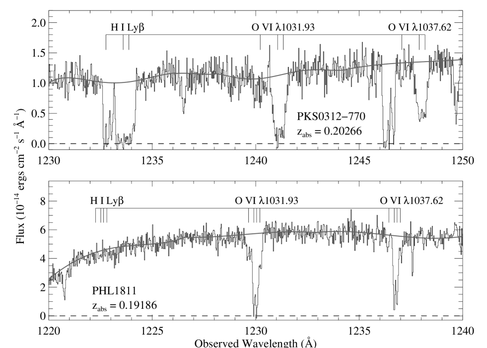
Figure 1.— Examples of strong O VI absorbers detected in STIS E140M echelle spectra of low$-$redshift QSOs. Small portions of the flux-calibrated echelle spectra of PKS0312-770 (upper panel) and PHL1811 (lower panel) are plotted versus heliocentric observed wavelength, and in both panels, the bar with tick marks indicates the centroids of components detected in the O VI $\lambda\lambda$1031.92, 1037.62 doublet as labeled. The thick gray lines indicate our adopted continuum placement in the vicinity of lines of interest. Toward PKS0312-770, a strong O VI system is detected at $z_{\rm abs}$ = 0.20266, and toward PHL1811 a multicomponent O VI absorber is found at $z_{\rm abs}$ = 0.19186. The tick marks also show the positions of the corresponding H I Ly$\beta$ absorption regardless of whether it is detected.

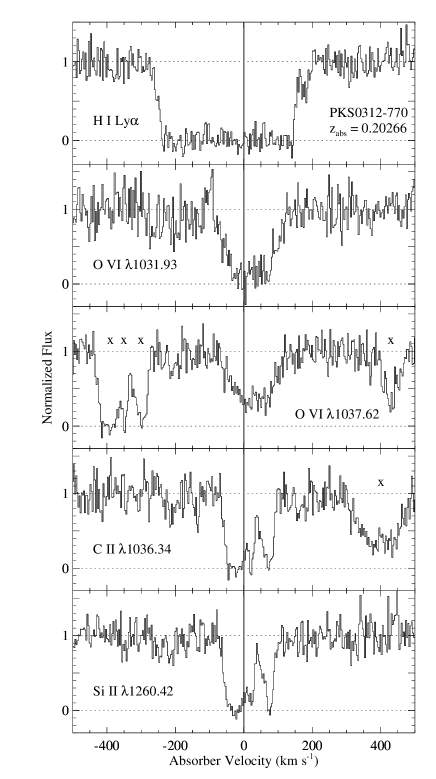
Figure 2.— Left: Examples of continuum-normalized absorption profiles detected in the intervening O VI absorber at $z_{\rm abs}$ = 0.20266 in the spectrum of PKS0312-770, including the H I Ly$\alpha$, O VI $\lambda\lambda$1031.93, 1037.62, C II $\lambda$1036.34, and Si II $\lambda$1260.42 transitions, as labeled. Unrelated lines are marked with crosses. Right: Examples of analogous absorption profiles detected in the proximate O VI absorption system at $z_{\rm abs}$ = 0.19186 toward PHL1811.

Figure 3.— Comparison of the detailed absorption profiles of the O VI $\lambda$1037.62 (top), C II $\lambda$1036.34 (middle), and Si II $\lambda$1260.42 (bottom) lines detected at $z_{\rm abs}$ = 0.20266 toward PKS0312-770. For purposes of comparison, the vertical dashed lines indicate the approximate velocity extent of the O VI absorption profile, and the heavy tickmarks indicate the velocity centroids of the three primary components evident in the low-ion profiles.

However, we can check for unresolved saturation by comparing the “apparent” column density profiles (Savage & Sembach 1991; Jenkins 1996) of two or more transitions of a species with significantly different $f\lambda$ values. To construct an apparent column density profile, we first calculate the apparent optical depth $\tau_{\rm a}(v)$ in each pixel of an absorption profile as a function of velocity,

$$\tau_{\rm a}(v)={\rm ln}\left[\frac{I_{\rm c}(v)}{I_{\rm ob}(v)}\right],$$ (1)

where $I_{\rm c}(v)$ is the estimated continuum intensity in the pixel at velocity $v$ and $I_{\rm ob}(v)$ is the observed intensity in that same pixel. To estimate the continuum shape and intensity, we fit a low-order Legendre polynomial fitted to line-free regions of the spectrum in the $\pm 1000$ km s^-1 interval centered on the absorption line of interest. The apparent column density is then determined from the apparent optical depth,

$$N_{\rm a}(v)=\frac{m_{e}c}{\pi e^{2}}\ \frac{\tau_{\rm a}(v)}{f\lambda}=3.768\times 10^{14}\ \frac{\tau_{\rm a}(v)}{f\lambda},$$ (2)

where $f$ is the oscillator strength and $\lambda$ is the wavelength of the transition, and the other symbols have their usual meanings. The numerical coefficient in eqn. 2 requires a wavelength measured in Å and produces an $N_{\rm a}(v)$ profile in atoms cm^-2 (km s^-1)^-1. $N_{\rm a}(v)$ is a representation of the true column density profile broadened by the instrument line spread function. If the line is fully resolved by the instrument, then $N_{\rm a}(v)$ can be integrated to determine the total column density. Even if the line is not well-resolved, the total column can still be measured reliably provided that the profile is not significantly affected by unresolved saturation. If two or more lines with log $f\lambda$ differing by 0.3 dex or more are compared and the $N_{\rm a}(v)$ profiles are found to be in agreement, then the profiles are not badly affected by saturation and can be integrated to measure the total column density, $N_{\rm total}=\int N_{\rm a}(v)dv$. If, conversely, the $N_{\rm a}(v)$ profiles are affected by saturation, then weaker lines will indicate higher apparent columns than their corresponding stronger lines in the velocity range affected by saturation. Apparent column density profiles have additional virtues as we will discuss in §3.4.

Since direct integration does not separate blended components, we list the total column densities, integrated across all components within an absorption feature, in Table 2. For the measurements of individual component properties, we employ the Voigt profile fitting code developed by Fitzpatrick & Spitzer (1997) with the STIS E140M line-spread functions from the STIS Handbook (Kim Quijano et al. 2003). We fit all transitions from a particular species (e.g., the O VI $\lambda$1031.93 and $\lambda$1037.62 transitions) simultaneously and obtain a single set of velocity centroids, column densities, and Doppler parameters for the components in the profiles of that species. Different species (e.g., H I vs. O VI or C III vs. O VI) can exist in separate gas phases and therefore are fitted independently. Table 3 lists the velocity centroids, Doppler parameters ($b-$values), and column densities of individual components detected in each O VI absorption system (some O VI absorbers show only one component, but many of the systems have multiple components). For cross referencing with the profile-fitting results, column 6 in Table 2 lists the number of components that are identified within each H I and O VI profile and their velocity centroids. Voigt profile fitting is a valuable measurement technique, but it is important to recognize the limitations and systematic uncertainties inherent in the method. Components that are free from blending, or components that are within blends but have a distinctive and well-constrained Gaussian shape in optical depth, are generally well-constrained by profile fitting. However, many components are revealed by well-detected but strongly blended inflections and profile asymmetries, and extra components that fit profile inflections/asymmetries are sometimes required to obtain an acceptable fit. Profile-fitting results for such blended components can be sensitive to the number of components selected to fit the profile. In these cases, the main (strongest) components are usually well-constrained, but the parameters of the “inflection” components can be sensitive to the number of components chosen for the fit. Components that are poorly constrained due to problems such as severe blending with adjacent components, significant saturation of all available lines, or low S/N are marked with a colon in Table 3. However, it is important to bear in mind that fitting results for complex multicomponent profiles can change considerably if more (or fewer) components are used in the fit. As emphasized by Spitzer & Fitzpatrick (1995) and Fitzpatrick & Spitzer (1997), the parameter uncertainties estimated by this Voigt profile fitting code increase appropriately when components are strongly blended, but the code cannot fully account for typical sources of systematic error. In our analyses below, we will consider how additional systematic uncertainties could affect our results.

2.3.2 Alignment of O VI and H I Components

In our previous papers on low$-z$ O VI absorbers, we have found that some O VI and H I components are remarkably well-aligned, and in some cases the narrow width of the aligned H I indicates a surprisingly low temperature (e.g., Tripp & Savage 2000; Lehner et al. 2006; Tripp et al. 2006a). We will revisit this aspect of the O VI systems with the larger sample of this paper in §4.1.1. We quantitatively identify aligned components based on the velocity difference between the O VI and H I component centroids, $\Delta v$(H I-O VI), and the uncertainty in that velocity difference, $\sigma(\Delta v)$. We calculate $\sigma(\Delta v)$ by combining the uncertainties in the O VI and H I component velocity centroids (from Table 3) in quadrature along with a term ($\sigma_{\rm wavecal}$) to account for the uncertainy in the wavelength scale calibration: $\sigma(\Delta v)=\sqrt{\sigma_{\rm O~{}VI}^{2}+\sigma_{\rm H~{}I}^{2}+\sigma_{\rm wavecal}^{2}}$. As noted above, the STIS and FUSE data have uncertainties in the wavelength-scale zero points as well as the relative wavelength calibration across the wavelength range of the observations. We bootstrap calibrated the FUSE data by comparing similar lines in the FUSE and STIS spectra, and this procedure reduces the FUSE zero-point uncertainty to $\approx 5$ km s^-1. When comparing O VI and H I components from STIS data only, we adopt $\sigma_{\rm wavecal}$ = 2 km s^-1 (based on the relative wavelength accuracies from the STIS Handbook), and when comparing components measured from STIS and FUSE data, we use $\sigma_{\rm wavecal}$ = 5 km s^-1. If an O VI and H I component pair have $\Delta v$(H I-O VI) $<2\sigma(\Delta v)$, we consider the components to be aligned. In the majority of the absorbers, the component matching is unambiguous: only one H I component is aligned with an O VI component within the 2$\sigma$ velocity difference uncertainty, or the H I and O VI components are simply not aligned. However, in a very small number of cases, an O VI component is aligned with two H I components to within the 2$\sigma$ uncertainties. In these cases, we use the components with the smallest $\Delta v$(H I-O VI) for our analysis, but we discuss how such ambiguities could affect the results. In our analysis of aligned O VI and H I components, we only use the measurements that are robust; we exclude the components that are marked with a colon in Table 3 because those measurements suffer from large uncertainties for various reasons (see Appendix).

For convenience, we number the components in each absorption system in column 8 of Table 3, and we indicate whether the O VI and H I components are aligned or offset from each other. If the components are aligned, we give the H I and O VI components the same number, and if a component is offset, it is given a unique number. For example, in the 3C 249.1 system at $z_{\rm abs}$ = 0.24676, we identify two H I components at $v=-79\pm 3$ km s^-1 (component 1) and $v=0\pm 1$ km s^-1 (component 2), and we find one O VI component at $v=0\pm 3$ km s^-1. The O VI component is aligned with H I component 2, and thus the O VI component is also identified as component 2. By using the same component numbers for aligned H I and O VI cases, the reader can easily identify which components are matched together from Table 3.

2.4. Absorber Classification

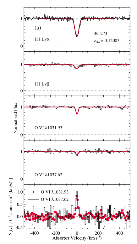
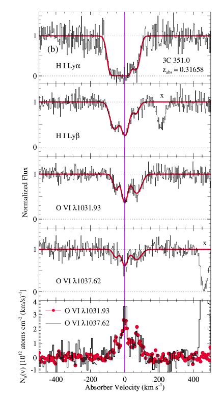
Figure 4.— Examples of continuum-normalized absorption profiles (black lines) of H I and O VI absorption lines detected in intervening absorbers. Voigt-profile fits are overplotted with a red line. The bottom panel in each stack shows the apparent column density profiles (see §2.3) of the O VI $\lambda 1031.93$ transition (red histogram + gray dots) and O VI $\lambda 1037.62$ line (black histogram). The panels show the following systems: (a) the 3C 273.0 absorber at $z_{\rm abs}$ = 0.12003, (b) the 3C 351.0 absorber at $z_{\rm abs}$ = 0.31658, (c) the H1821+643 absorber at $z_{\rm abs}$ = 0.26656, and (d) the PG1216+069 absorber at $z_{\rm abs}$ = 0.12360.

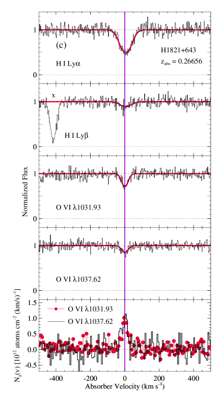
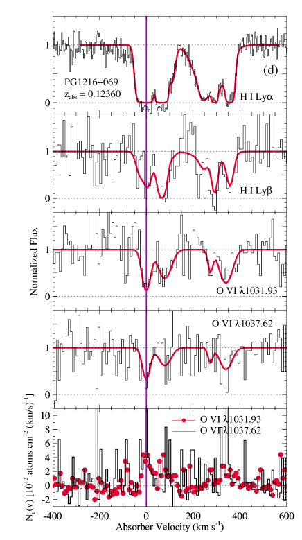
Figure 4.— continued.

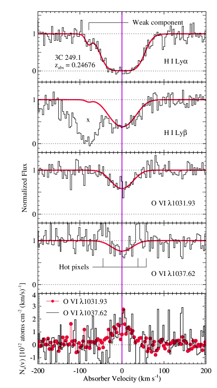
Figure 6.— Example of an O VI absorber in which the O VI and H I are well-aligned with the exception of a weak, outlying component detected only in the Ly$\alpha$ profile. Apart from the labeled weak H I component at $v=-79$ km s^-1, the O VI and H I profiles are quite similar. Given the range of H I/O VI ratios found in O VI systems, any O VI associated with the weak component is likely to be undetectable at this signal-to-noise level. We classify this absorber as “simple*” (§2.4.1) to indicate that the majority of the O VI and H I profiles are well-aligned and can be analyzed as a single-phase system. As in Figure 4, the lowest panel compares the $N_{\rm a}(v)$ profiles of the O VI $\lambda\lambda$1031.93,1037.62 lines, and unrelated lines from other redshifts are marked with an $\times$. Note that several hot-pixel features that are not readily removed are located near the O VI $\lambda$1037.62 line.

Figure 7.— Velocity offsets between H I and O VI components in intervening absorbers measured in simple (single-phase) systems (hatched thin line) and complex (multiphase) absorbers (thick line). Each O VI component is matched with the H I component that is closest in velocity in order to calculate the velocity difference.

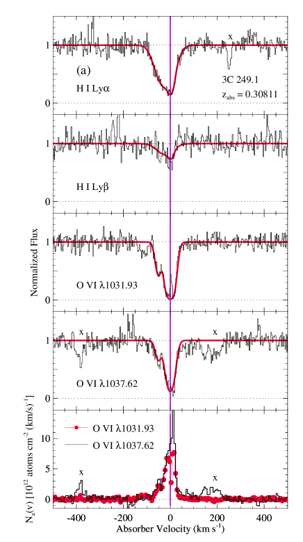
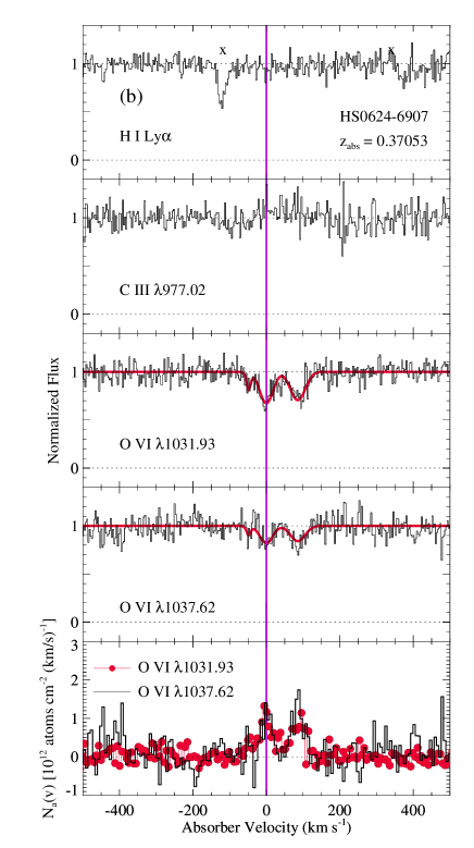
Figure 8.— Examples of continuum-normalized absorption profiles (black lines) of H I and O VI absorption lines detected in proximate absorbers (i.e., absorption systems located within 5000 km s^-1 of the QSO redshift); the symbols and line colors are analogous to those in Figure 4. The panels show the following systems: (a) the 3C 249.1 absorber at $z_{\rm abs}$ = 0.30811, (b) the HS0624+6907 absorber at $z_{\rm abs}$ = 0.37053, (c) the PG0953+415 absorber at $z_{\rm abs}$ = 0.23351, and (d) the TON28 absorber at $z_{\rm abs}$ = 0.33021.

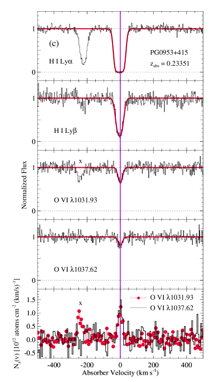
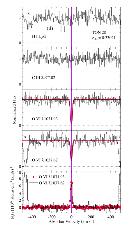
Figure 7.— continued.

2.4.1 Single-Phase/Simple vs. Multiphase/Complex Absorbers

It is useful to classify the low$-z$ O VI absorbers in various ways. To motivate the classifications used in this paper, we begin with some examples of the absorption-line systems that demonstrate their diverse characteristics and categories. Two examples of strong O VI absorbers identified in our STIS spectra are shown in Figure 1. This figure shows small portions of the STIS spectra of PKS0312-770 and PHL1811 covering O VI systems at $z_{\rm abs}$ = 0.20266 and 0.19186, respectively. The examples in Figure 1 demonstrate the tremendous diversity of low$-z$ O VI absorbers: from Tables 2 and 3, we see that the O VI column densities are similar in these PKS0312-770 and PHL1811 systems, but the $N$(H I)/$N$(O VI) ratio is ostensibly $\gtrsim 10^{4}$ times larger in the PKS0312-770 example. This can partially be seen by comparing the paucity of H I Ly$\beta$ absorption in the PHL1811 case to the strongly saturated, multicomponent Ly$\beta$ profile in the PKS0312-770 system. There are several reasons that O VI absorbers can show such a large range in the H I/O VI ratio. First, when good constraints are available, it has been shown that the metallicities of apparently intergalactic, low$-z$ QSO absorbers span a large range from $Z=0.02-0.06Z_{\odot}$ (e.g., Tripp et al. 2002, 2005) up to $Z=0.5-1.0Z_{\odot}$ (e.g., Savage et al. 2002; Prochaska et al. 2004; Jenkins et al. 2005; Aracil et al. 2006). If the metallicity varies by a factor of 50, the H I/O VI ratio will vary by a similar ratio. Second, the H I/O VI ratio is very sensitive to the ionization conditions. As we will discuss in detail in §4, in collisional ionization equilibrium, for example, relatively small changes in the gas temperature can lead to large changes in the H I/O VI ratio. Similarly, in photoionized gas, small changes in the gas density, ionizing flux, or ionizing radiation field shape can lead to substantial changes in the H I/O VI ratio. Third, many of the O VI absorbers are multiphase absorbers. Lower-ionization phases can substantially increase the H I absorption strength without increasing the O VI strength at all.

Indeed, looking more closely at the examples in Figure 1, we can find strong evidence that multiphase effects contribute to the huge difference in the H I/O VI ratios in these particular cases. Figure 2 shows the continuum-normalized absorption profiles of selected H I, O VI, C II, and Si II transitions in the PKS0312-770 and PHL1811 absorbers. Strong, multicomponent C II and Si II absorption is clearly detected in the PKS0312-770 system, but these low ions are not evident in the PHL1811 absorber. Moreover, the profiles of the C II and Si II lines in the PKS0312-770 case are quite similar to each other with at least three distinct components, two of which are relatively narrow. Figure 3 shows a closer look at some of the PKS0312-770 metal lines (over a smaller velocity range). From this figure, we immediately see that the O VI component structure differs from the low-ion component structure. The O VI absorption extends over a similar velocity range but does not show the three distinct components seen in C II and Si II. This indicates either that the O VI lines originate in a different phase or that additional components are present in the O VI profile that blend together and smear out the component structure; either explanation requires at least some of the O VI absorption to arise in separate phases from the low ions. The former explanation is more natural: if the O VI absorption arises in hotter gas (as expected since it peaks in abundance at $T\approx 10^{5.5}$ K in collisionally ionized gas), its Doppler parameter $b$ will be broader ($b=\sqrt{2kT/m}$, where $T$ is the temperature and $m$ is the atomic mass) and the O VI components would hence be more blended as seen in Figure 3. It is worthwhile to note that some high-velocity clouds (HVCs) in the vicinity of the Milky Way have similar characteristics to the profiles shown in Figure 3, i.e., O VI and low-ion absorption spread over the same velocity range but with somewhat different centroids and/or line widths (see, e.g., Sembach et al. 2003; Tripp et al. 2003; Fox et al. 2004,2006; Ganguly et al. 2005; Collins et al. 2007).

It is not surprising to conclude that O VI and low-ion lines originate in different phases; this is expected intuitively because these species exist mainly in very different temperature ranges in collisionally ionized gas in equilibrium (e.g., Bryans et al. 2006). A more surprising result is that we also find that a substantial fraction of our O VI absorbers show similar O VI and H I profiles suggestive of single-phase clouds. We show four examples of intervening O VI absorbers in Figure 4. In these four examples, we detect both O VI and H I with good significance, and the O VI and H I lines are well-aligned and have similar shapes. In these aligned systems, the H I/O VI ratio varies significantly from one system to the next (and the ratio even varies among components within a single absorber as, e.g., in the $z_{\rm abs}$ = 0.31658 system toward 3C 351.0), but it is critical to notice how the O VI and H I centroids are well-aligned in velocity, and the profile shapes are quite similar (but are not identical). This suggests that the O VI and H I originate in a single gas phase in these cases and provides an important constraint on the physical conditions of the gas (as we will discuss further in §4).

Motivated by the mixture of evidence regarding the number of phases in the O VI absorbers, we have classified the O VI systems as either (1) “simple” absorbers that are entirely composed of aligned H I and O VI componenents (as defined in §2.3.2), which suggests that the components could be single-phase absorbing entities, and (2) “complex” systems that show significant velocity offsets between low-ionization and high-ionization lines, which indicates that these absorbers are multiphase systems. These classifications are listed in column 2 of Table 3. In a few absorbers, the primary components are aligned in the O VI and H I profiles, but weak components are detected in H I that do not show corresponding O VI. An example of such a system is shown in Figure 6. In this absorber in the spectrum of 3C 249.1, we see that the main component at $v=0$ km s^-1 is well-aligned in H I and O VI, but an additional, rather weak H I component that shows no O VI is evident at $v=-79$ km s^-1. The H I Ly$\alpha$ transition is very sensitive to low-density, low-$N$(H I) gas, and when $N$(H I) is very low, it is likely that any associated O VI absorption is simply too weak to be detected at the S/N level of our data. In cases where the bulk of the H I and O VI absorption is aligned but weak H I components are present with no corresponding O VI (as in Figure 6), we classify the absorber as a simple case, but we mark the system with an asterisk in Table 3 to note the presence of weak H I without corresponding O VI. In some instances, the H I profiles and component centroids are poorly constrained, e.g., if the absorber is a black Lyman-limit system presenting only badly saturated Lyman series lines or if H I is not detected at all (as found in several systems near the QSO redshifts); in these cases, we list the classification as uncertain. In the intervening absorber sample, we classify 37% of the absorbers as simple (single-phase) systems and 53% as complex (multiphase) systems (10% have uncertain classifications).

To show the quantitative distinction between the simple (single-phase) and complex (multiphase) intervening absorbers, we show in Figure 7 the velocity offsets between H I and O VI components, $\Delta v$(H I - O VI) $=v_{{\rm H~{}I}}-v_{{\rm O~{}VI}}$. For this figure, we match each O VI component with the H I component that is closest in velocity. For this figure only, all O VI components are matched with an H I component, including cases where there are more O VI components than H I components (in these cases, multiple O VI components are paired with the same H I line). Systems that have uncertain classification are excluded from Figure 7, and components that are significantly uncertain due to problems such as blending and saturation (components marked with a colon in Table 3) are also excluded. From this figure, we see that there is a clear kinematical distinction between simple/single-phase and complex/multiphase absorbers: some of our O VI absorbers are characterized by highly-aligned O VI and H I components, but an equally large fraction of the intervening systems have more complex relationships between H I and O VI with significantly different kinematics. We will return to this distinction below.

2.4.2 Intervening vs. Proximate/Intrinsic Absorbers

We classify the absorbers a second way for an orthogonal purpose: we list in column 2 of Table 3 whether the system is classified as an intervening absorber (Int) or a proximate absorber (Prox). It has long been recognized that some of the so-called “associated” absorption systems (often called “proximate” absorbers in the recent literature) close to the redshift of the background QSO ($z_{\rm abs}\approx z_{\rm QSO}$) have a fundamentally different nature from intervening absorbers that arise in the IGM or ISM of foreground objects (e.g., Lynds 1967; Burbidge 1970; Foltz et al. 1986). The “broad-absorption line” (BAL) QSOs are easily recognized by their dramatic P Cygni-like absorption troughs with outflow velocities approaching a substantial fraction of the speed of light (see, e.g., Turnshek 1988), but apart from BAL QSOs, there is a statistical excess of metal-bearing absorbers within $\approx$ 5000 km s^-1 of $z_{\rm QSO}$ (Foltz et al. 1986) that in many regards look like the ordinary, narrow absorption lines that arise in foreground galaxies and the IGM. However, evidence such as temporal variability (on timescales of a few years) and/or incomplete covering of the background flux source indicates that at least some “narrow” absorption lines originate in material located quite close to the QSO itself (see, e.g., Hamann 1997; Yuan et al. 2002; Ganguly et al. 2003, and references therein).

Following the seminal work of Weymann et al. (1979) and Foltz et al. (1986), narrow absorption lines found within 5000 km s^-1 of the QSO redshift are usually classified as associated (proximate) absorbers, and we adhere to this standard definition in this paper (however, in some cases we show how the measurements change if we change the velocity cutoff for the proximate absorber classification). The velocity of displacement $v_{\rm displ}$ must account for relativistic effects but can be easily determined from the QSO and absorber redshifts using the usual $\beta$ formula,

$$\beta=\frac{v_{\rm displ}}{c}=\frac{(1+z_{\rm QSO})^{2}-(1+z_{\rm abs})^{2}}{(1+z_{\rm QSO})^{2}+(1+z_{\rm abs})^{2}}.$$ (3)

We also distinguish between associated absorbers and “mini-BAL” systems. Mini-BALs show many of the characteristics of BALs but are spread over a smaller velocity range (e.g., Barlow et al. 1997). One of our sight lines (3C 351.0) shows a clear example of a mini-BAL with strong evidence that the absorption lines arise in intrinsic material close to the QSO. This is clearly a different type of absorption system, and we do not include it in our samples. A full analysis of the 3C 351.0 mini-BAL has been presented by Yuan et al. (2002).

However, the 5000 km s^-1 velocity interval used to define proximate absorbers corresponds to a relatively large Hubble-flow distance, and it is inevitable that some truly intervening absorbers will be classified as associated just because they are located in the 5000 km s^-1 region of space near the QSO; indeed, Sembach et al. (2004) show examples of this problem (see their §10). On the other hand, compelling direct evidence of narrow absorption systems associated with the QSO with $v_{\rm displ}\gg$ 5000 km s^-1 has been found at high redshifts; Hamann, Barlow, & Junkkarinen (1997) reported clear temporal variability and partial coverage of the flux source in an absorber displaced by $\approx$24,000 km s^-1 from the emission redshift of Q2343+125 ($z_{\rm QSO}$ = 2.24), for example. Based on statistical excesses of absorbers observed toward different types of QSOs, Richards et al. (1999,2001) have argued that up to 36% of C IV absorbers at $z_{\rm abs}\sim$ 2.5 with 5000 $\leq v_{\rm displ}\leq$ 75,000 km s^-1 arise in ejected material intrinsic to the background QSO. More recently, Misawa et al. (2007) have searched for partial coverage in narrow metal-line absorbers detected in high-resolution Keck spectra of 37 high$-z$ QSOs, and they conclude that $10-17$% of narrow C IV absorbers are intrinsic (associated with the QSO) in the 5000 $\leq v_{\rm displ}\leq$ 75,000 km s^-1 interval.

Evidently, displacement velocity might not provide a straightforward means of distinguishing between intervening and intrinsic absorbers. The absorbers that are usually referred to as associated systems are a mixture of intervening and intrinsic absorbers. To avoid the confusing connotations of the term “associated”, in this paper we will follow recent papers (e.g., Ellison et al. 2002; Russell et al. 2006; Hennawi & Prochaska 2007) and refer to any absorber with $v_{\rm displ}\leq$ 5000 km s^-1 as a “proximate” absorber regardless of its nature/origin, but we use “intrinsic” to connote that the system is physically close to the QSO. It is important to bear in mind the possible confusion that intrinsic systems could cause in samples of intervening systems defined based on $v_{\rm displ}$. Because nearby galaxy redshifts are more straightforwardly measured, an advantage of low$-z$ samples is that if $10-30$% of the systems in the $5000-75,000$ km s^-1 interval are intrinsic/ejected, we should find that this fraction of the metal systems are randomly distributed with respect to the foreground galaxies. Studies of correlations between metal systems and foreground galaxies so far have not found any evidence of randomly distributed metal systems; instead, the metal absorbers appear to be clearly correlated with galaxies (e.g., Savage, Tripp, & Lu 1998; Tripp & Savage 2000; Savage et al. 2002; Sembach et al. 2004; Tumlinson et al. 2005; Prochaska et al. 2006; Stocke et al. 2006; Williger et al. 2006; Aracil et al. 2006; Tripp et al. 2006a). We are currently expanding the sample of sight lines for low$-z$ galaxy-absorber correlation analyses, but this investigation will be presented in a separate paper. In this paper, however, we will search for any evidence that some of the O VI absorbers at 5000 $\leq v_{\rm displ}\leq$ 75,000 km s^-1 have characteristics that indicate an ejected/intrinsic origin. We will find that in our sample, ejected/intrinsic systems appear to be predominantly confined to $v_{\rm displ}\lesssim$ 2500 km s^-1 (see §3).

Figure 10.— Example of the sensitivity of our STIS E140M data. The top panel shows the STIS E140M spectrum of 3C 249.1, binned to $\approx$35 km s^-1 pixels to show the continuum shape and emission lines clearly. QSO broad emission lines are labeled in parentheses underneath the spectrum. The bars and tickmarks show the locations of the intervening O VI absorbers at $z_{\rm abs}$ = 0.23641 and 0.24676 as well as the proximate O VI systems at $z_{\rm abs}$ = 0.30811 and 0.31364. For each system, the ticks indicate the redshifted wavelengths of the C III $\lambda$977.02, H I Ly$\beta$, O VI $\lambda\lambda$1031.93, 1037.62, and H I Ly$\alpha$ lines from left to right, respectively. The thick bars are the intervening cases; the thin bars mark the proximate systems. The lower panel shows the 3$\sigma$ limiting equivalent width obtained by integrating the full-resolution data over 15-pixel windows. The sawtooth pattern in the limiting equivalent width is due to the blaze function of the echelle grating, which causes the S/N of the spectrum to vary significantly across a given echelle order. This is mitigated in some regions because adjacent echelle orders overlap, and coaddition of the overlapping regions offsets the lower S/N at the edges of the echelle orders. The large positive spikes are due to strong interstellar or intergalactic absorption lines, which block portions of the spectrum and prevent the detection of weak extragalactic lines within the wavelength range of the strong absorption profile. The measured equivalent widths of the detected O VI $\lambda$1031.93 lines in the intervening and proximate O VI systems are shown with filled circles and open squares, respectively, in the lower panel.

Figure 8 shows several examples of the proximate O VI absorbers that we have identified in the 16 sight lines studied in this paper. This figure shows that some of the proximate systems have characteristics that are quite similar to those of the intervening systems. For example, the proximate absorbers of 3C 249.1 (at $z_{\rm abs}$ = 0.30811) and PG0953+415 ($z_{\rm abs}$ = 0.23351) have strong H I lines as well as O VI, and the H I and O VI lines are well-aligned. However, some of the proximate systems have very weak affiliated H I absorption. The HS0624+6907 and TON28 proximate systems in Figure 8 are two examples of proximate systems with very weak H I. In several cases, H I is not detected at all despite good S/N. As noted in the previous section, some intervening systems show substantial velocity offsets between the H I and O VI absorption, but intervening systems almost always show some detectable H I absorption in the vicinity of the O VI. As we will discuss further below, one unique characteristic of the proximate systems is that some show no affiliated H I absorption whatsoever. Using the same classification criteria discussed above, we categorize 21% of the proximate absorbers as “simple” systems composed of O VI and H I components that are aligned, and 50% of the proximate systems are complex.

3. Statistics

3.1. Number of O VI Absorbers per Unit Redshift

We now turn to the statistical properties of the intervening and proximate absorbers presented in Tables 2 and 3. We begin with the number of O VI absorbers per unit redshift, $dN/dz$. This is a fundamental quantity that characterizes the various types of QSO absorbers. Moreover, it is straightforward to use theoretical models and simulations to predict $dN/dz$ for O VI absorbers (e.g., Cen et al. 2001; Fang & Bryan 2001; Chen et al. 2003; Furlanetto et al. 2005; Tumlinson & Fang 2005; Cen & Fang 2006), and measurement of $dN/dz$ provides an important test of the validity of these large-scale cosmological models.

3.1.1 $dN/dz$ Measurement Method and Uncertainties

To estimate $dN/dz$ for a sample of absorbers with equivalent widths greater than a specified limiting equivalent width $W_{\rm lim}$, we simply tabulate the number of O VI systems detected with $W_{\rm r}\geq W_{\rm lim}$ and divide by the total path $\Delta z$ over which we were able to search for the absorbers. However, there are a few minor complications in this simple calculation. First, the S/N ratios of our spectra are not completely uniform; some sight lines have higher over S/N ratios than others, and even along a single sight line, some wavelength regions have higher S/N. Second, some redshifts are blocked by strong Galactic ISM lines or unrelated extragalactic lines. These blocked regions reduce the total $\Delta z$ that is effectively searched for absorption systems. The total $\Delta z$ and number of absorbers in a given sample must carefully account for the variable S/N and blocking of the spectra. For example, suppose that a line with $W_{\rm r}=$ 150 mÅ is detected in a spectral region with S/N that is only sufficient to detect lines with $W_{\rm r}\geq$ 100 mÅ. That region would not be included in the total $\Delta z$ for a sample with $W_{\rm r}\geq$ 30 mÅ, and thus the 150 mÅ line cannot be counted in a $W_{\rm r}\geq$ 30 mÅ sample. However, this absorber would be included in a sample with $W_{\rm r}\geq$ 100 mÅor larger.

To account for the variable S/N of the data and blocking by unrelated lines, we calculate for each sight line the rest-frame $3\sigma$ limiting equivalent width at each observed wavelength $\lambda$ where O VI absorbers can be detected,

$$W_{\rm lim}(\lambda)=\frac{3\sigma_{W(\lambda)}}{1+z_{\rm abs}},$$ (4)

where $\sigma_{W(\lambda)}$ is the total uncertainty in an equivalent width integrated over some number of pixels. For a single pixel $i$, the equivalent width uncertainty $\sigma_{W(i)}$ is

$$\sigma_{W(i)}=\Delta\lambda(i)\left[\frac{\sigma_{I(\lambda_{i})}}{I(\lambda_{i})}\right],$$ (5)

where $\Delta\lambda(i)$ is the pixel width, $I(\lambda_{i})$ is the flux in pixel $i$, and $\sigma_{I(\lambda_{i})}$ is the $1\sigma$ flux uncertainty in pixel $i$. However, both the STIS and FUSE data have at least two pixels per resolution element, and in fact, all of the clearly detected O VI lines are spread over at least several 2-pixel resolution elements. Therefore, to evaluate $W_{\rm lim}(\lambda)$, we must integrate over $n$ pixels,

$$\sigma_{W(\lambda)}^{2}=\sum_{i=1}^{n}\sigma_{W(i)}^{2}.$$ (6)

For a given limiting equivalent width, we have empirically determined the number of pixels to integrate over based on the detected O VI lines with measured equivalent widths close to the limiting equivalent width of interest (see further details below). After $W_{\rm lim}(\lambda)$ has been evaluated over the full range of O VI coverage for all 16 sight lines, we evaluate $\Delta z$ for various samples of lines with strengths greater than $W_{\rm r}$ by summing the total redshift path over which $W_{\rm lim}(\lambda)\leq W_{\rm r}$. We first check for detectability of the O VI $\lambda$1031.93 line when evaluating the total $\Delta z$. When O VI $\lambda$1031.93 is redshifted into a region blocked by a strong ISM or extragalactic line, our algorithm checks whether the corresponding O VI $\lambda$1037.62 can be detected instead. O VI $\lambda$1037.62 is redshifted to a different observed wavelength, and the different observed $\lambda$ usually places $\lambda$1037.62 outside of the blocked region. However, because of its lower $f\lambda$ value, the O VI $\lambda$1037.62 is expected to be a factor of two weaker than $\lambda$1031.93, so when checking the corresponding $\lambda$1037.62 region, we require $W_{\rm lim}(\lambda)\leq 0.5W_{\rm r}$ in order to add to the total $\Delta z$ (e.g., if we cannot detect a 30 mÅ O VI $\lambda$1031.93 line, we have to be able to detect a 15 mÅ O VI $\lambda$1037.62 line instead). In this way, we estimate the total path over which we can detect either O VI $\lambda$1031.93 or O VI $\lambda$1037.63. This approach also accounts for regions with steep S/N gradients (e.g., in the vicinity of the broad QSO emission lines) that might make one line of the doublet detectable while the other lines falls below the detection threshold.

Figure 10 shows an example of the resulting limiting equivalent width calculated for equivalent widths greater than 30 mÅ for the STIS observations of 3C 249.1. The top panel of Figure 10 shows the 3C 249.1 STIS spectrum (binned to $\approx$ 35 km s^-1 pixels to more clearly show the characteristics of the spectrum), and the lower panel shows the $3\sigma$ limiting equivalent width obtained by integrating over 15-pixel detection windows (15 full-resolution, unbinned pixels). Figure 10 shows several important characteristics of the data that deserve comment. First, the proper calculation of $W_{\rm lim}(\lambda)$ automatically corrects for portions of the spectra that are blocked by strong interstellar or extragalactic lines. In these regions, the S/N drops precipitously and $W_{\rm lim}(\lambda)$ increases accordingly; if neither the $\lambda 1031.93$ line nor the $\lambda 1037.62$ line falls in a region with sufficient sensitivity, then that redshift window does not contribute to the total $\Delta z$. In addition, when moderate strength lines are present, $W_{\rm lim}(\lambda)$ increases, but these locations can add to $\Delta z$ for samples of stronger lines. For example, a contaminating 150 mÅ ISM line might effectively hide a 30 mÅ extragalactic O VI line, but it would not hide a 300 mÅ O VI line, and this is properly evaluated using this approach. Second, the S/N and $W_{\rm lim}(\lambda)$ are not uniform across a STIS E140M spectrum for several reasons. The STIS E140M sensitivity peaks at $\lambda_{\rm obs}\approx$1340 Å and decreases at shorter and longer wavelengths. However, superimposed on this broad and slowly-varying sensitivity is a sawtooth pattern due to the blaze function of the echelle grating: within each echelle order, the S/N decreases significantly when moving away from the blaze peak. This is partly mitigated in regions where adjacent orders overlap; in these overlapping regions, coaddition of the two orders recovers some of the lost signal-to-noise. Given these various effects, it is clear that the limiting equivalent width is a complicated array that is not easily approximated by a simple function. However, our method fully accomodates the various sources of sensitivity variations.

As can be seen from Figures 1-7 and Tables 2-3, many of the O VI systems show multiple (often blended) components spread over 200$-$500 km s^-1 intervals. The way that the individual components within these blends are counted introduces another source of uncertainty in $dN/dz$ measurements. For example, the O VI absorber at $z_{\rm abs}$ = 0.31658 toward 3C 351.0 shows three blended (but clearly detected and distinct) components at $v_{\rm abs}$ = $-51,0,$ and 70 km s^-1 (see Figure 4). Does this case count as one or three absorption systems? These velocity differences correspond to a substantial distance in a pure Hubble flow, and it is conceivable that the three components in this example arise in gas associated with three discrete galaxies. But, the three components could alternatively be due to three clouds within the surroundings of a single galaxy. Published theoretical $dN/dz$ predictions often do not specify how the absorbers how counted, and indeed, the appropriate method likely depends on the purpose of the $dN/dz$ measurement. This issue has greatest impact on our $dN/dz$ measurements for O VI absorbers with the largest equivalent widths; these cases are rare and almost always show evidence multiple components, so spliting the high-$W_{\rm r}$ cases into several lower-$W_{\rm r}$ cases reduces $dN/dz$ for the highest $W_{\rm r}$ bins. To show how this issue affects our results, we report two separate $dN/dz$ measurements. We estimate $dN/dz$ for systems, in which we count multiple components that are contiguously connected with each other as a single O VI case, and we also determine $dN/dz$ for components where every identified individual component is counted as a separate case.

3.1.2 $dN/dz$ Results: Cumulative Distribution

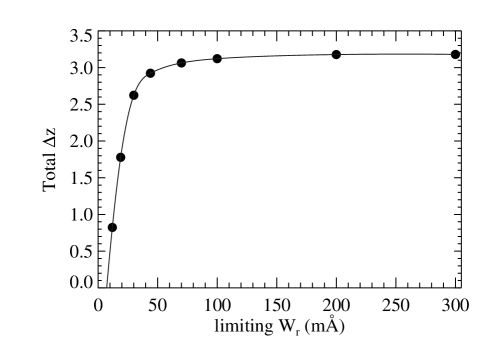
Figure 11.— The total path ($\Delta z$) over which the 16 QSO sight lines have sufficient signal-to-noise ratio to detect intervening O VI lines with rest-frame equivalent width $W_{\rm r}\geq$ limiting $W_{\rm r}$, calculated as described in §3.1. The total $\Delta z$ was explicitly calculated at the points indicated by filled circles, and the solid line shows a spline fit that is used to interpolate to find $\Delta z$ at values between the filled circles.

In Table 4, we report our $dN/dz$ measurements for intervening O VI absorbers for samples with $W_{\rm r}>$ 30, 70, 100, 200, and 300 mÅ. To determine the limiting equivalent equivalent width and total $\Delta z$ for these bins (as described in §3.1.1), we integrate over 15, 22, 30, 50, and 70 STIS pixels, respectively. For convenience, after explicitly calculating $\Delta z$ for these specific limiting $W_{\rm r}$ values, we fitted cubic spline functions to the $\Delta z$ vs. limiting $W_{\rm r}$ data. The total $\Delta z$ values and the cubic spline fit for the intervening absorbers are shown in Figure 11. For each intervening sample, Table 4 lists the number of O VI systems identified, the total path $\Delta z$ over which we could detect an O VI $\lambda$1031.93 line with $W_{\rm r}$ greater than the limiting value of that sample, and the implied $dN/dz$ found by counting either systems (column 4) or components (column 5) as explained above.

Table 5 lists the same quantities but for the proximate O VI absorbers. As discussed above, typically associated/proximate absorbers are defined in the literature to be any system with $v_{\rm displ}<5000$ km s^-1, so we derive $dN/dz$ assuming this standard definition, and the results are shown in the upper half of Table 5. However, we will show below that the excess of proximate O VI systems for our sight lines appears to be confined to the $-1000\lesssim v_{\rm displ}\lesssim 2500$ km s^-1 interval, so we also list in Table 5 the results that we obtain by alternatively defining proximate systems to be those found with $v_{\rm displ}\leq 2500$ km s^-1. In Tables 4 and 5, we use the Gehrels (1986) small-sample tables to estimate the statistical uncertainties in $dN/dz$.

We now offer several comments on our $dN/dz$ measurements; we compare these results to theoretical predictions in §3.1.4. We begin by comparing our intervening absorber measurements to the O VI $dN/dz$ results reported by Danforth & Shull (2005; see also Danforth et al. 2006). Danforth & Shull (2005) have conducted a search for O VI lines at $z_{\rm abs}<0.15$ in the spectra of 31 active galactic nuclei observed with FUSE. For their $dN/dz$ calculation, Danforth & Shull (2005) count each component as a separate case (see Table 3 in Danforth et al. 2006), so we should compare our component $dN/dz$ results to the Danforth & Shull (2005) measurements. Comparing the numbers in column 5 of Table 4 to the analogous quantities from Danforth & Shull’s Table 1, we see that the $dN/dz$ measurements from the two papers agree within the reported $1-2\sigma$ uncertainties. However, our $dN/dz$ measurements are systematically higher than those of Danforth & Shull (2005) by roughly $0.1-0.3$ dex.

We can identify several reasons why we find systematically higher $dN/dz$ values than Danforth & Shull (2005) for intervening O VI systems including the following: (1) Danforth & Shull (2005) only searched for O VI affiliated with absorption systems that have H I Ly$\alpha$ lines with equivalent widths greater than 80 mÅ. In our sample, on the other hand, we include all O VI absorbers regardless of the strength of the corresponding H I Ly$\alpha$ line. From Table 2, we see that we do find O VI absorbers with weak corresponding Ly$\alpha$ lines with $W_{\rm r}$(Ly$\alpha$) $<$80 mÅ. Our inclusion of these weak-Ly$\alpha$ O VI absorbers increases $dN/dz$ compared to the results of Danforth & Shull (2005). (2) We do not classify any absorbers within 5000 km s^-1 of the QSO redshift as an intervening absorber, while Danforth et al. (2006) use 1800 km s^-1 as the cutoff for intervening vs. proximate absorbers. The Danforth & Shull proximate absorber definition results in a larger $\Delta z$ searched for intervening O VI per sight line, and since we do not find many O VI lines in the $1800\leq v_{\rm displ}\leq 5000$ km s^-1 interval (see below), this has the net effect of increasing $\Delta z$ palpably without increasing the total number of systems much. Using the 1800 km s^-1 cutoff therefore decreases $dN/dz$. If we were to adopt the Danforth & Shull proximate absorber cutoff, our $dN/dz$ measurements would decrease by 0.03 dex. (3) Danforth & Shull integrate over a single resolution element in order to determine their limiting equivalent width. Since very few (if any) of our detected O VI systems are completely unresolved and spread over a single resolution element, we choose to integrate over a larger number of pixels to determine $W_{\rm lim}$ as discussed above. This results in higher $W_{\rm lim}$ in our sample and a lower total $\Delta z$ over which our data have sufficient S/N to reveal an O VI system of a given strength. If we were to also integrate over a single resolution element, our $\Delta z$ values would increase and our $dN/dz$ numbers would decrease. This issue is most important for the samples that include the weakest lines (e.g., the $W_{\rm r}\geq$ 30 mÅ sample). Individually, these three factors have small effects on the measured $dN/dz$, but they all change $dN/dz$ in the same direction when comparing our results to those of Danforth & Shull (2005). The combined effect of these three issues can easily account for the systematic difference between our findings and those of Danforth & Shull (2005).

Figure 12 compares our O VI $dN/dz$ measurements to analogous measurements for low$-z$ C IV absorbers from Frye et al. (2003) and low$-z$ Mg II systems from Churchill et al. (1999) and Narayanan et al. (2005). All of the measurements in Figure 12 were derived from low$-z$ samples ($z_{\rm abs}<0.6$) except for the Mg II measurement from Churchill et al. (1999), which was derived from a sample extending to moderately higher redshifts ($0.4\leq z_{\rm abs}\leq 1.4$). O VI, C IV, and Mg II are the most commonly studied metals in optically-thin QSO absorption systems, and we see from Figure 12 that O VI lines have a substantially higher number per unit $z$ at low redshifts than either the Mg II absorbers or the C IV systems. This is not surprising in the case of Mg II; this species is easily photoionized by the UV background from QSOs, and it is likely to be present only when an absorber has a relatively high H I column density. However, it is interesting to note that $dN/dz$ of O VI is substantially higher than $dN/dz$ of C IV. Because C IV is often redshifted outside of the Ly$\alpha$ forest, it is by far the most studied metal in the high-redshift regime, and it would be valuable to compare the low$-z$ C IV absorbers to their high$-z$ analogs. It is unfortunate that for our low$-z$ O VI absorber sample, the C IV doublet is usually redshifted beyond the long-wavelength cutoff of our observations. However, IGM ionization models can be constrained by the different $dN/dz$ trends for O VI and C IV shown in Figure 12.

From Tables 4-5 and Figure 12, we also see that statistically, the O VI $dN/dz$ increases substantially when the absorber redshift range is close to the background QSO redshift (compare the open squares and filled circles in Figure 12). Using the standard $v_{\rm disp}<5000$ km s^-1 definition of proximate absorbers, we find that there are 2$-$6 times more proximate O VI systems per unit $z$ than intervening O VI systems (we find similar results comparing $dN/dz$ of individual components instead of $dN/dz$ of O VI systems). As we have already noted, the excess of O VI lines appears to be largely confined to a smaller velocity interval ($v_{\rm displ}<2500$ km s^-1) closer to the QSO redshift than the standard 5000 km s^-1 definition (see further discussion below). If we use the 2500 km s^-1 velocity cutoff to define the proximate absorbers, we find an even more dramatic excess: in this case, there are $3-10$ times more proximate O VI systems per unit redshift than we find in the intervening sample. The magnitude of the proximate absorber excess depends on the sample limiting equivalent width, and it is worth noting that the excess is greatest when comparing the stronger O VI lines.

It is of interest to assess whether a convenient function, such as a power law, can be fitted to the O VI $dN/dz$ data shown in Figure 12. As shown in Figure 12, for the system $dN/dz$ results, an inverse variance-weighted power law of the form log $dN/dz$ = $\alpha\ {\rm log}\ W_{\rm lim}+constant$ provides a satisfactory fit for both the intervening and proximate O VI measurements with $\alpha$(intervening) = $-1.00$ and $\alpha$(proximate) = $-0.69$. However, we can also see from Figure 12 that for the intervening systems, the slope of the observed log $dN/dz$ vs. log $W_{\rm lim}$ data appears to change at $W_{\rm lim}<$ 70 mÅ. To show this, we also plot in Figure 12 the power law obtained by fitting only the bins with $W_{\rm lim}\geq$ 70 mÅ. Exclusion of the 30 mÅ bin results in a steeper slope and clearly improves the fit to the higher equivalent width bins. This type of turnover is sometimes interpreted as evidence of incompleteness, i.e., the measured $dN/dz$ is lower than the true $dN/dz$ because the data were inadequate to detect all of the absorbers in the weakest $W_{\rm r}$ bin. We argue that this explanation is unlikely to explain the change in slope apparent in our O VI measurements. We have corrected for incompleteness by carefully calculating the total $\Delta z$ path over which 30 mÅ lines can be detected. In principle, we could have overestimated $\Delta z$, e.g., by integrating equation 6 over an insufficient number of pixels, which in turn would underestimate $dN/dz$. However, this is an unlikely explanation because we would have to overestimate $\Delta z$ by an unreasonable amount to reconcile the intervening O VI data with the steeper power law shown in Figure 12. Figure 12 shows the results and fits for O VI systems; as shown in Table 4, if we count components instead of systems, the $dN/dz$ vs. $W_{\rm lim}$ slope steepens significantly (single strong systems split up into multiple weaker components). Power-law fits to the component $dN/dz$ measurements are acceptable for the proximate absorbers, but we find that a single power law provides a rather poor description of the $dN/dz$ measurements for the intervening O VI components.

3.1.3 $dN/dz$ Results: Differential Distribution

In the previous section we discussed the cumulative $dN/dz$ distribution of O VI absorbers. We show the differential O VI $dN/dz$ distribution for intervening and proximate absorbers in Figure 13 as a function of $N$(O VI) using 0.2 dex bins extending from log $N$(O VI) = 13.2 to 14.8. In Figure 13, we show the $dN/dz$ that results from counting individual components, and we exclude the marginal measurements (those marked with a colon in Table 3). The total path ($\Delta z$) for each column density bin is from Figure 11. As discussed in §3.1.1, we calculate $\Delta z$ as a function of limiting equivalent width. To estimate $\Delta z$ for a limiting column density, we converted $W_{\rm lim}$ to $N_{\rm lim}$ assuming the median $b-$value found for the intervening and proximate absorbers (see §3.2): $b$ = 24 km s^-1 for intervening absorbers, and $b$ = 16 km s^-1 for proximate systems.

Figure 12.— Measurements of the cumulative number of QSO absorbers per unit redshift ($dN/dz$) for O VI, C IV, and Mg II absorbers with $1\sigma$ statistical uncertainties. The O VI measurements are from this paper (see Tables 4 and 5), the C IV results are from Frye et al. (2003), and the Mg II numbers are from Narayanan et al. (2005) and Churchill et al. (1999). For the O VI systems, $dN/dz$ is plotted for both the intervening systems (filled circles) and the proximate absorbers found within 2500 km s^-1 of the QSO redshift (open squares; as shown in Table 5, the proximate system $dN/dz$ decreases if we use $v_{\rm displ}<5000$ km s^-1 as the cutoff). In this figure, we show $dN/dz$ for O VI systems (see text §3.1.1). All of these measurements are for systems at $z_{\rm abs}<0.6$ except for the Churchill et al. point (the higher Mg II $dN/dz$), which was derived from a somewhat higher redshift sample ($0.4\leq z_{\rm abs}\leq 1.4$). The dotted lines show power-law fits, weighted by inverse variance, to the intervening O VI absorbers using all of the measurements (thin dotted line) and using all of the measurements except the 30 mÅ point (thick dotted line). The dashed lines show analogous power-law fits for the proximate absorbers.

Figure 13.— The differential O VI $dN/dz$ distribution for intervening absorber components (thick line) and proximate absorber components with $v_{\rm displ}<5000$ km s^-1 (thin line). The differential $dN/dz$ is shown in 0.2 dex bins for log $N$(O VI) $\geq$ 13.2.

3.1.4 Comparison with Theoretical $dN/dz$ Predictions for Intervening Absorbers

Most theoretical studies of the low$-z$ O VI absorbers have made predictions regarding the cumulative $dN/dz$ distribution, so we focus on the cumulative distribution in our comparison to theoretical work. It is not clear if there is a physical motivation for fitting the $dN/dz$ data in Figure 12 with a power law. Some theoretical papers have argued that $dN/dz$ vs. $W_{\rm lim}$ should turn over as $W_{\rm lim}$ decreases. For example, Tumlinson & Fang (2005) suggest that this turnover could be a result of the processes that transport metals out of galaxies. They argue that if galaxies can only pollute metals into limited volumes in their immediate vicinities, then $dN/dz$ should turnover as observed. In their recent survey of low$-z$ O VI absorber environments, Stocke et al. (2006) find no O VI systems in galaxy voids, which is consistent with the Tumlinson & Fang (2005) hypothesis.

Cosmological simulations also predict a $dN/dz$ turnover. Several papers have employed hydrodynamic simulations of large-scale structure growth to predict the number of O VI absorbers per unit redshift for various samples of intervening absorbers defined by the limiting equivalent width. We compare these theoretical predictions to our measurements in Figure 14. The earlier predictions of Cen et al. (2001) are superseded by the more recent predictions of Cen & Fang (2006), so we do not show the Cen et al. (2001) predictions in Figure 14. Also, Chen et al. (2003) and Cen & Fang (2006) have presented predictions for multiple models that make different assumptions about, e.g., the processes that transport metals out of galaxies, nonequilibrium ionization effects, and the overall level and scatter of the IGM metallicity. Current cosmological simulations have limited ability to fully model complicated processes such as metal transport, and it should be borne in mind that significantly uncertain assumptions are sometimes required to predict statistics of metal absorption line systems from hydrodynamic simulations. For this reason, we do not show the predictions of individual models in Figure 14 but instead use hatched regions to show the range of $dN/dz$ predictions for intervening O VI systems from several theoretical papers, i.e., the lower envelope of the hatched region shows the lowest prediction from the indicated paper, and the upper envelope indicates the highest prediction.

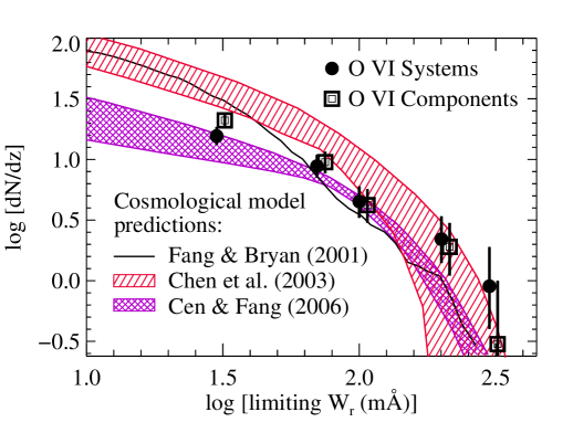
Figure 14.— Comparison of the observed number of intervening O VI absorbers per unit redshift ($dN/dz$) from this paper to the predictions of hydrodynamic cosmological simulations from Fang & Bryan (2001, solid black line), Chen et al. (2003, red hatched region), and Cen & Fang (2006, purple hatched region). These theoretical predictions apply to $z\approx 0$. The observations are indicated by points with $1\sigma$ statistical error bars; filled circles show the results obtained by counting blended components as a single “system”, and double squares show the $dN/dz$ measurements found by counting each component (including components that are close in velocity and blended) as a separate case. Chen et al. (2003) and Cen & Fang (2006) present a variety of models that vary the physics implementations and assumptions. The hatched regions indicate the range of $dN/dz$ predicted by their models.

As we have already noted, it is not always clear how the O VI absorbers are counted in the cosmological simulation papers. Chen et al. (2003) note that they do not attempt to deblend blended lines, so for comparison to their predictions, the system $dN/dz$ measurements from column (4) of Table 4 should be employed. Other simulation papers employ Voigt-profile fitting (e.g., Fang & Bryan 2001), so for those predictions, the component $dN/dz$ should be used. In Figure 14, we show the measurements of the O VI redshift density counting systems (filled circles) and components (double squares). Overall, we see broad but imperfect agreement between the simulation predictions and the observations. The simulations predict that the $dN/dz$ distribution should turnover with decreasing $W_{\rm lim}$ as observed. The Chen et al. (2003) models predict too many O VI systems at $W_{\rm lim}\lesssim 70$ mÅ but roughly agree with the observations at higher equivalent width limits. The Cen & Fang (2006) model that results in the highest O VI redshift density (i.e., their model that includes galactic superwinds but neglects nonequilibrium ionization effects) agrees with the measurements for weak O VI systems but underpredicts the observed number of relatively strong O VI absorbers. It is not surprising that the models and observations do not agree in detail because the physical processes that are relevant (e.g., metal transport) are very challenging to model, and approximate assumptions are required. Bearing this in mind, the rough agreement between the models and the observations is encouraging.

3.2. Doppler Parameter and Column Density Distributions

Figure 15.— The distribution of O VI $b-$values measured in individual components from Voigt-profile fitting (see Table 3). The thick lines show the measurements in intervening systems, and the thin lines show the proximate absorber measurements (with $v_{\rm displ}<$ 5000 km s^-1). Marginal measurements (those flagged with a colon in Table 3) are excluded from this plot. The $b-$value for O VI at $T=3\times 10^{5}$ K (where O VI peaks in abundance in CIE) is 18 km s^-1.

Are the physical conditions implied by the O VI observations consistent with the expectations from the cosmological simulations? To address this question, we now examine the implications of the detailed O VI line measurements. We begin by comparing the Doppler parameter and column density distributions of the intervening and proximate absorber components. Our motivation for this comparison is twofold: First, considering the findings and issues noted in §2.4.2, we would like to search for differences in the properties of intervening and proximate absorbers that might be useful for recognizing ejected/intrinsic absorbers at high displacement velocities. Second, the proximate absorbers are highly likely to be photoionized. Some proximate systems show evidence that they are located close to the QSO central engine (see §2.4.2) where photoionization by the intense UV emission from the QSO is likely to be dominant. Even if the proximate absorbers arise in an entirely different galaxy from the QSO host, they are still likely to be predominantly photoionized by the QSO light because the Stromgren spheres of luminous QSOs can extend over large distances/redshift intervals (e.g., Zheng & Davidsen 1995; Smette et al. 2002). Therefore proximate absorbers provide a valuable photoionized control sample for understanding the ionization of the intervening systems.

We have noted in Table 3 that some of the individual component measurements are more uncertain due to systematic problems such as strong blending and line saturation. We evaluate the effects of including or excluding these uncertain cases by defining two samples. Our “robust” sample excludes the uncertain cases that are flagged with a colon in Table 3, and the “full” sample uses all of the measurements (including the highly uncertain cases). Table 6 summarizes some basic measurements for these samples including the median and mean values of the O VI column densities and $b-$values and the number of components in each sample. Inspecting Table 6, we see that the mean and median O VI column densities of the intervening and proximate absorbers are similar, with the intervening absorbers having somewhat lower columns on average. Comparing the $b-$values, we notice that the proximate systems tend to be somewhat narrower than then intervening cases. To statistically test whether the intervening and proximate absorbers have different $N$(O VI) and $b$ distributions, we have applied Kolmogorov-Smirnov (KS) tests. Table 6 lists the results of our KS tests comparing the column density and $b-$value distributions of the proximate and intervening samples. Comparing the column-density distributions of the robust intervening and proximate absorbers with a KS test, we find the KS statistic $D=0.171$ and the probability of the null hypothesis (i.e., that the intervening and proximate absorbers are drawn from the same parent distribution) is 55.8% . Therefore we find no compelling evidence that the intervening and proximate absorbers have different column density distributions. If we use the full sample instead of the robust sample, we reach the same conclusion.

We have also used a KS test to compare the differential $dN/dz$ distribution of the intervening and proximate O VI components shown in Figure 13. By comparing the differential $dN/dz$ distributions instead of the straight column-density distributions, we account for possible differences in the sensitivity of the spectra used to search for intervening vs. proximate absorbers. By definition, proximate absorbers are located near the peak of the Ly$\beta$ + O VI emission line of the background QSO, and consequently, the proximate absorbers are found in regions where the flux is elevated and the S/N ratio is higher. Thus, the proximate absorber regions can reveal weaker lines than the regions probed for intervening systems. However, a KS test applied to the differential $dN/dz$ distributions shown in Figure 13 indicates a 49.7% probability that the samples are drawn from the same parent distribution, so there is no statistically significant difference between the intervening and proximate absorbers.

The mean and median $b-$values of the proximate absorbers are lower than those of the intervening lines. The proximate and intervening absorber $b-$value distributions are compared in Figure 15. Applying the KS test to the robust intervening and proximate $b-$value distributions, we find that the probability that the two samples are drawn from the same parent distribution is 3.6% . This weakly suggests that the intervening and proximate absorbers have different $b-$value distributions, but the result is only marginally significant. The full sample yields a KS probability of 5.3 %, i.e., a similar result.

However, as we have discussed, the $v_{\rm displ}<$ 5000 km s^-1 definition of the proximate absorbers may be somewhat arbitrary, and the truly intrinsic absorbers might be mostly confined to a smaller velocity interval closer to $z_{\rm QSO}$. In Table 6, we show the mean and median statistics obtained by defining proximate absorbers to be those cases with $v_{\rm displ}<$ 2500 km s^-1. We see that this alternative definition only results in a slightly lower median and mean column densities and $b-$values. However, the probability that the intervening and proximate $b-$values have the same distribution decreases if we use the $v_{\rm displ}<$ 2500 km s^-1 definition: the probability of the null hypothesis decreases to $1.6-2.7$%. Thus, we find a somewhat stronger indication that the proximate absorbers are statistically more narrow than the intervening lines with the hypothesis that proximate/intrinsic systems are predominantly confined to $v_{\rm displ}<$ 2500 km s^-1.

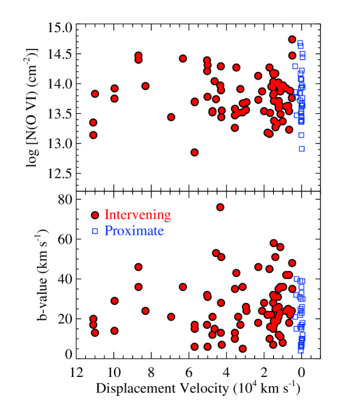
Figure 16.— Upper panel: Individual-component O VI column densities as a function of velocity of displacement from the QSO redshift, $v_{\rm displ}=c[(1+z_{\rm QSO})^{2}-(1+z_{\rm abs})^{2}]/[(1+z_{\rm QSO})^{2}+(1+z_{\rm abs})^{2}]$, for intervening components (red filled circles) and proximate systems within 5000 km s^-1 of the QSO redshift (blue open squares). Lower panel: O VI $b-$values vs. displacement velocity for intervening and proximate absorbers.

Is there any direct evidence that the absorber distributions and properties change at some value of $v_{\rm displ}$? Or, is there evidence that a substantial fraction of the proximate/intrinsic absorbers are dispersed to large displacement velocities and are intermingled with the intervening systems as suggested by some of the papers noted in §2.4.2? In Figure 16, we show the O VI column densities and $b-$values of the intervening absorbers (filled circles) and the proximate systems (open squares) as a function of $v_{\rm displ}$. While some intrinsic systems with high $v_{\rm displ}$ have been reported in the literature (§2.4.2), the majority of the known intrinsic systems are found relatively close to redshift of the QSO. Therefore, we might expect the absorber properties to change as $v_{\rm displ}$ approaches zero (i.e., as $z_{\rm abs}$ approaches $z_{\rm QSO}$) if there are a significant number of intrinsic systems at $v_{\rm displ}<5000$ km s^-1. This would be manifested as a correlation between $N$(O VI) or $b$(O VI) and $v_{\rm displ}$. However, we have used Spearman tests to evaluate this hypothesis, and we find that there are no statistically significant correlations of any combination of the data shown in Figure 16. Considering only the intervening absorbers, we find that $N$(O VI) and $b$(O VI) are not correlated with $v_{\rm displ}$. Likewise, the proximate absorbers show no significant correlations. Finally, combining the intervening and proximate systems into a single sample, we find no compelling correlations.

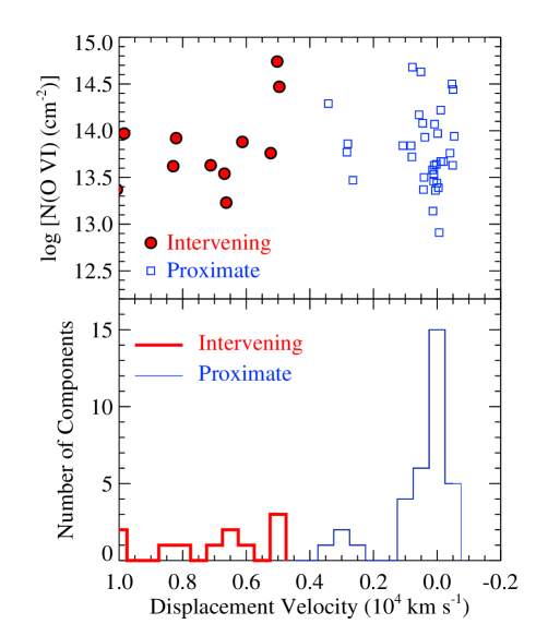
Figure 17.— Upper panel: Invidual-component O VI column densities vs. displacement velocity (as in Figure 16 but expanded to more clearly show the absorbers within 10,000 km s^-1 of the QSO redshift). Lower panel: Number of O VI components detected in 500 km s^-1 displacement-velocity bins extending from $v_{\rm displ}=-2000$ km s^-1 to $+10,000$ km s^-1. The thick line shows the systems formally classified as intervening, and the thin line shows the proximate systems. A substantial excess of absorption lines is clearly evident within $\approx$1000 km s^-1 of the QSO redshifts.

Ostensibly, Figure 16 does show an apparent increase in the simple number of intervening O VI lines at $v_{\rm displ}\lesssim 6\times 10^{4}$ km s^-1. However, this is not a real effect. Because of the combination of QSO redshifts and the observed wavelength range of the various spectra, some of the sight lines probe larger ranges of $v_{\rm displ}$ than others. All of the sight lines cover the $v_{\rm displ}\approx$ 0 km s^-1 region, but the upper bound on the observed $v_{\rm displ}$ range varies significantly among the sight lines. Consequently, the number of lines detected thins out as $v_{\rm displ}$ increases because fewer sight lines cover the larger $v_{\rm displ}$ values.

We do notice, however, that the distribution of proximate absorber velocities is sharply peaked around $v_{\rm displ}\approx 0$ km s^-1. This is a real effect since all of the sight lines fully cover the $-2000\leq v_{\rm displ}\leq 5000$ km s^-1 range. To show this more clearly, we show in the lower panel of Figure 17 the number of O VI lines found in 500 km s^-1 bins in the $-2000\leq v_{\rm displ}\leq 10000$ km s^-1 range; the thick-line histogram shows the intervening systems, and the thin-line histogram represents the proximate cases (assuming the $v_{\rm displ}\leq 5000$ km s^-1 definition). For reference, the upper panel of Figure 17 shows the column densities of the individual components that contribute to each bin in the lower panel. We see that for $v_{\rm displ}\gtrsim 1500$ km s^-1, all of the bins, intervening or proximate, have $0-3$ counts. At $v_{\rm displ}<1500$ km s^-1, however, the number of counts in each bin increases dramatically with 15 components in the bin centered at $v_{\rm displ}=0$ km s^-1 and $4-6$ counts in the other three bins. There is clearly a substantial excess of O VI lines at $v_{\rm displ}<1500$ km s^-1. The excess is also evident in the contrasting $dN/dz$ measurements listed in Tables 4 and 5. This excess is similar to the excess of C IV absorption lines at $v_{\rm displ}\approx 0$ km s^-1 observed at higher redshifts (e.g., Foltz et al. 1986). Apparently, the standard $v_{\rm displ}$ value used to classify proximate absorbers (i.e., $v_{\rm displ}<5000$ km s^-1) could be too large; the majority of the truly intrinsic absorbers appear to be located at smaller displacement velocities. There are known proximate systems at $z_{\rm abs}<0.4$ with intrinsic absorption lines identified at $v_{\rm displ}\gg 1500$ km s^-1 (e.g., Yuan et al. 2002; Ganguly et al. 2003), but those systems have the characteristics of “mini-BAL” systems.

3.3. Correlation of $N$(O VI) with $b$(O VI)

Some theoretical studies have predicted that $N$(O VI) and $b$(O VI) should be highly correlated. Using the basic ideas and formalism of Edgar & Chevalier (1986), Heckman et al. (2002) have argued that a correlation of $N$(O VI) and $b$(O VI) is a natural consequence of radiative cooling in a wide variety of contexts, and they present a heterogeneous sample of O VI measurements that are consistent with the expected $N-b$ correlation. Heckman et al. (2002) include in their sample a small number of extragalactic O VI systems as well as measurements in the Milky Way ISM, the Magellanic Clouds, and starburst galaxies. Subsequently, Lehner et al. (2006) and Danforth et al. (2006) revisited the Heckman et al. model with more homogeneous samples that only included extragalactic O VI systems, and they report mixed results. Danforth et al. (2006) report that they find no correlation between $N$(O VI) and $b$(O VI). Conversely, Lehner et al. (2006) present a sample of measurements that are generally consistent with the Heckman et al. models, but they note that the models predict Ne VIII columns that are too large compared to their observations.

Using our sample of component measurements from Table 3, Figure 18 plots log $N$(O VI) vs. $b$(O VI). As in previous sections, we show both the intervening and proximate systems (with $v_{\rm displ}<$ 5000 km s^-1) with filled circles and open squares, respectively. The dashed line in Figure 18 indicates the locus of $N$(O VI) and $b$(O VI) values for a single Gaussian line with a central optical depth of 10% . Lines that are broad and have a low column density are difficult or impossible to detect because the optical depth in individual pixels in their absorption profiles are comparable to (or less than) the noise in the continuum. Moreover, such lines are difficult to distinguish from undulations in the intrinsic continuum of the QSO. Consequently, this $N-b$ locus is effectively a detection threshold; lines below the dashed line in Figure 18 are usually undetectable. Neglect of this factor can produce an artificial correlation, as can be seen from Figure 18. We have used Spearman tests to evaluate whether $N$(O VI) and $b$(O VI) measurements from this paper are correlated. To account for the detection threshold, we only use lines with log $N$(O VI) $\geq 13.6$ in the Spearman test; from Figure 18, we can see that we can detect lines with log $N$(O VI) $\geq 13.6$ over the full range of measured $b-$values. From Spearman tests, we find that the proximate absorbers are not significantly correlated using either the robust sample or the full sample. On the other hand, the Spearman test indicates that in the case of the intervening absorbers, $N$(O VI) and $b$(O VI) are correlated at the $2.7\sigma$ level.

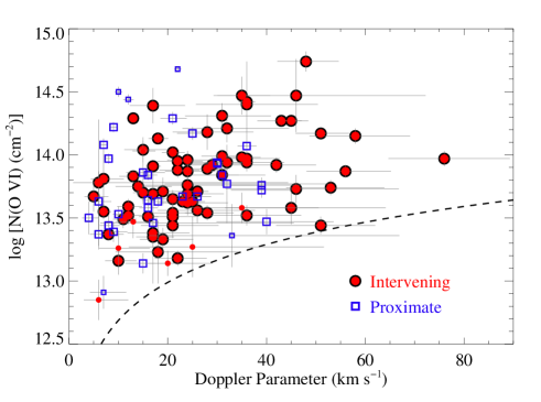
Figure 18.— The O VI column density and $b-$value combinations measured in individual components using Voigt-profile fitting (see Table 3). Filled red circles show measurements of the column densities and $b-$values of components in intervening systems, and open blue squares show the proximate absorber measurements. This figure shows all measurements reported in Table 3, but the measurements that are marginal (due to problems such as line saturation) are plotted with smaller symbols. The dashed line shows the locus of $b-$value - $N$(O VI) combinations for a Gaussian line with a central optical depth of 10% ; this is an approximate detection threshold for the data used in this paper.

While the correlation in the intervening sample is suggestive, its significance is insufficient to provide compelling support for the Heckman et al. (2002) model. Moreover, comparing our measurements to the predictions from Heckman et al. (see their Figure 1), we see that the scatter in the intervening absorbers is substantially larger than the scatter expected in the radiative cooling model. This may not be surprising because the intervening sample contains absorbers that are quite possibly photoionized (see §4) and would not be expected to have correlated values of $N$ and $b$. However, if we omit the absorbers that appear to be photoionized, the significance of the correlation remains marginal ($<3\sigma$). The intervening absorber sample considered here has a narrower range of $b$ and $N$ than the sample studied by Heckman et al. (2002). Their sample contained much larger columns and velocity widths since it included measurements of O VI absorption in starburst outflows. The correlation between $N$ and $b$ is strongest in these types of environments, and recent results seem to confirm that the trend at the higher end of the $N-b$ distribution persists (T. M. Heckman 2008, private communication). In such environments, collisional processes dominate, and radiative cooling is an important, perhaps dominant, process in establishing line profile shapes. While the simple Heckman et al. (2002) model may not reflect the O VI intervening absorber population characteristics in all cases, it is likely that radiative cooling contributes in part to the observed distribution of $N$ and $b$ values.

3.4. Profile Shapes: O VI vs. H I

The detailed correspondence (or lack thereof) between O VI and H I provides useful insight on the physical conditions and nature of the absorbers, so we now present comparisons of the O VI and H I profile shapes. In §2.4.1, we noted that some of the O VI absorbers are characterized by kinematical simplicity with all the O VI and H I component velocity centroids aligned to within their 2$\sigma$ uncertainties (§2.3.2), but other systems are more complex with velocity offsets between the nearest O VI and H I components that can exceed 50 km s^-1 (see Figure 7). When the H I and O VI centroids in a component are well-aligned, the component can be modeled as a single-phase gas cloud (conversely, significant velocity offsets preclude single-phase models). Additional information such as the low-ion profiles presented in §2.4.1 and Figure 3 (for the PKS0312-770 system at $z_{\rm abs}=0.20266$) can also establish that an absorber is a multiphase entity, and when available, we have used information on low ions to evaluate whether a system is truly a multiphase absorber.

As noted in §2.4, we classify 37% of the intervening absorbers as simple systems with all of their O VI and H I components aligned to within the measurement uncertainties. We can go beyond rough classifications and gain better insight by directly examining the O VI and H I profiles. To do this, we employ apparent column density $[N_{\rm a}(v)]$ profiles as described in §2.3. $N_{\rm a}(v)$ profiles have a significant advantage for comparing different species: $N_{\rm a}(v)$ profiles are linear functions, and they can be simply scaled to compare the detailed correspondence of two species. When good detections of multiple transitions are available for a given species (e.g., the 1031.93 and 1037.62 Å lines or multiple H I Lyman series lines), we use the method of Jenkins & Peimbert (1997) to construct composite $N_{\rm a}(v)$ profiles. These composite profiles have better S/N ratios. More importantly, weak lines can be used to constrain the $N_{\rm a}(v)$ profile in high-column density regions where the strong lines are saturated, and conversely, strong lines can be employed to flesh out the profile in the low-density regions where the weak lines are undetectable.

Figure 19.— Theoretical apparent column density profiles observed at the resolution of the STIS E140M echelle spectrograph (based on the E140M line-spread functions from the STIS Handbook for the $0\farcs 060\farcs 2$ slit). All of the profiles are normalized so that the peak of the profile = 1.0. The dashed line shows the profile of a marginally resolved line with $b$ = 4 km s^-1. The solid line shows the predicted profile for an O VI line broadened only by thermal motions and arising in gas at $T=3.0\times 10^{5}$ K, and the dotted line shows the corresponding H I profile, i.e., an H I line that is only broadened by thermal motions at $T=3.0\times 10^{5}$ K. At this temperature, O VI and H I lines are well-resolved with the E140M spectrograph and are expected to have dramatically different $N_{\rm a}(v)$ profiles if they are predominantly thermally broadened.

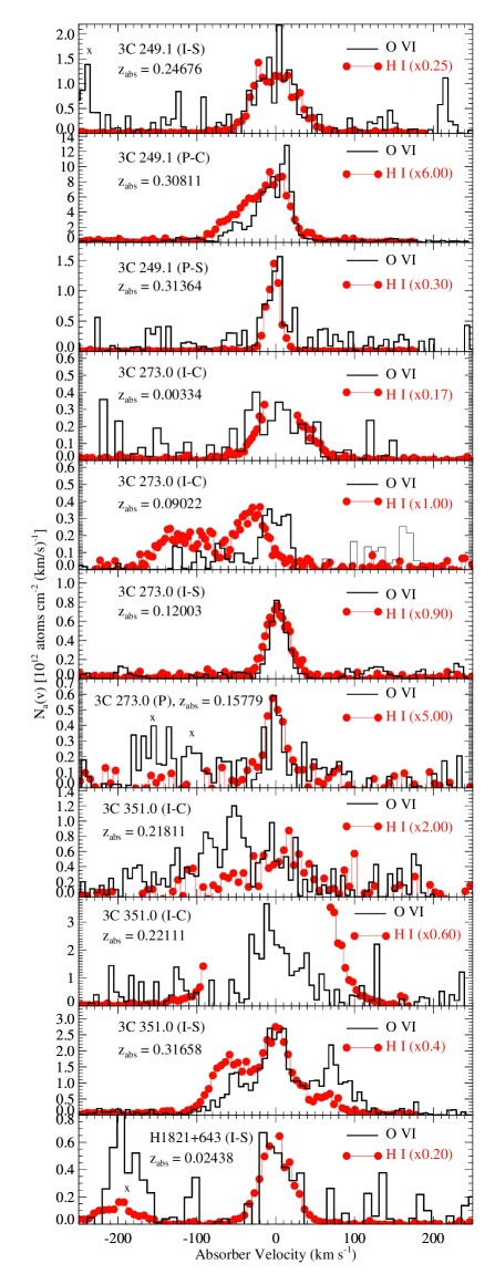
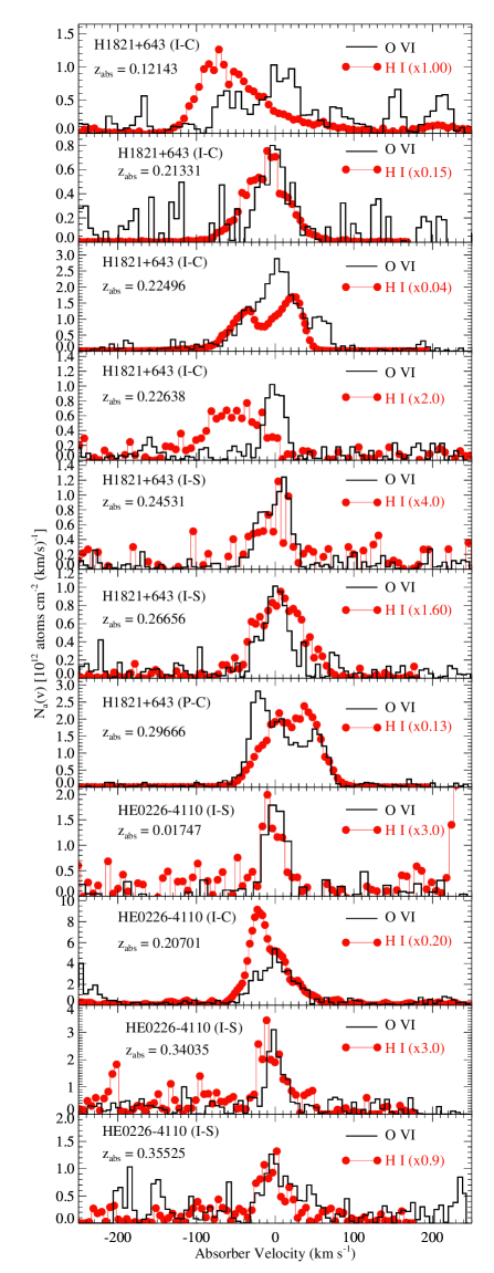
Figure 20.— Comparison of the O VI apparent column density profiles (black histograms) to the affiliated H I $N_{\rm a}(v)$ profiles (red-dot histograms) for all O VI absorbers reported in this paper. Each panel is labeled with the QSO sight line and the redshift of the system shown in that panel. Codes in parentheses denote whether the system is intervening (I) or proximate (P) and whether it is classified as simple (S) or complex (C). The H I profiles have been scaled as indicated in each panel for comparison with the O VI profile (the H I scale factors are not based on fits; these are just convenient scalings for purposes of comparison); in some cases a different scaling is shown with a small black-dot histogram. Whenever possible, the profiles are weighted composite profiles derived from multiple transitions using the method of Jenkins & Peimbert (1997). By constructing composite profiles, weaker lines can be used to determine $N_{\rm a}(v)$ in the line cores where the strong lines are saturated. However, in some cases, all available data are strongly saturated in some portion of the profile. In these cases, there are gaps in velocity ranges where all available data are saturated. In this figure, the STIS data are binned to 7 km s^-1 pixels and the FUSE data are shown with $\approx$10 km s^-1 pixels. Unrelated features are marked with “x”.

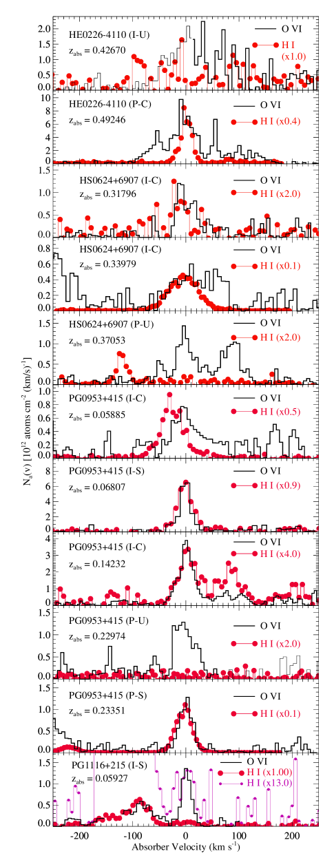
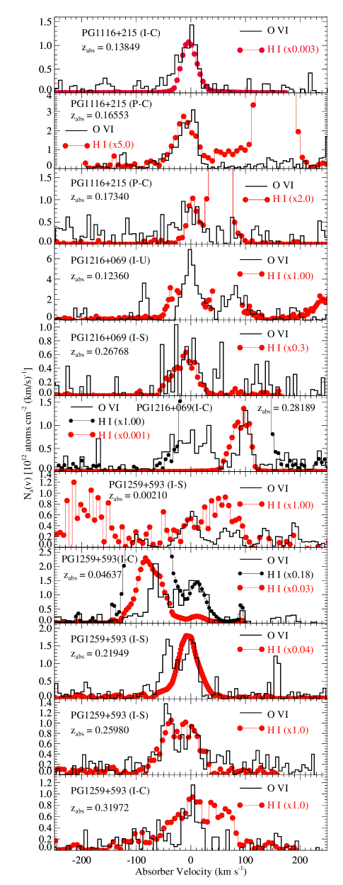
Figure 18.— continued

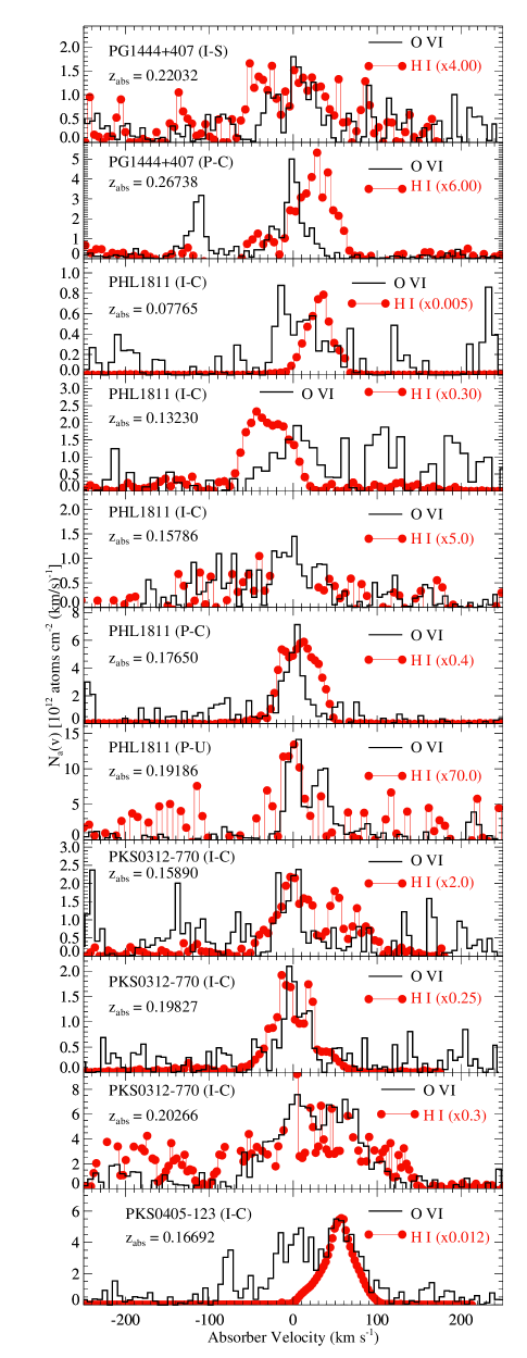
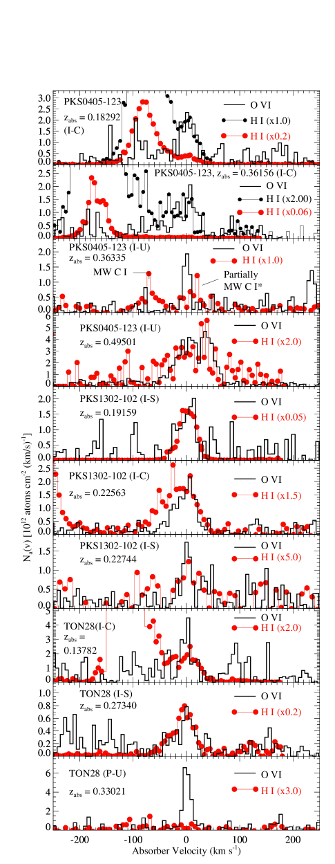
Figure 18.— continued

To guide the interpretation of the $N_{\rm a}(v)$ profiles, we show in Figure 19 several theoretical $N_{\rm a}(v)$ profiles constructed using the STIS E140M line-spread function (using the LSF for the $0\farcs 06\times 0\farcs 2$ slit). The E140M mode has excellent spectral resolution, and consequently, relatively narrow lines are resolved with this spectrograph. The dashed line in Figure 19 shows a marginally resolved, hypothetical line with $b=4$ km s^-1; the solid line shows a thermally broadened O VI profile at $T=3.0\times 10^{5}$ K [i.e., close to the temperature where O VI peaks in abundance in collisional ionization equilibrium (CIE)]. We can see that at this gas temperature, an O VI line is well-resolved, and the apparent column density profile is therefore a close approximation of the the true column density profile. The dotted line in Figure 19 shows the $N_{\rm a}(v)$ profile of a thermally broadened H I line, also at $T=3.0\times 10^{5}$ K, normalized to have the same peak value as the O VI line. Comparison of the O VI and H I profiles in Figure 19 makes an important point: because its mass is 16 times smaller, H I profiles should be four times broader than O VI lines arising in the same gas if the lines are predominantly thermally broadened. At the resolution provided by our STIS data, detection of this effect is, in principle, trivial at the temperatures expected for the WHIM gas. As we shall see, H I profiles that are significantly broader than the corresponding O VI profiles (like those shown in Figure 19) are relatively rare in the real data of our sample. We note that the sensitivity of our STIS data is sufficient to detect H I with good significance at the temperatures where O VI peaks in CIE (see, e.g., Richter et al. 2006a,b). However, there are some important caveats. As we will show in §4.2.1, if the temperature range is tuned to maximize the O VI/H I ratio or the absorber metallicity is intrinsically high, then a broad H I component corresponding with hot O VI could be quite difficult to detect. Also, in complex multicomponent systems, broad Ly$\alpha$ components are often easily hidden (§4.2).

The observed $N_{\rm a}(v)$ profiles derived from the O VI and H I lines for all of the absorbers (intervening and proximate) are shown in Figure 20. The profiles are ordered alphabetically by sight line name and presented sequentially by redshift for a given sight line. Following the sight line name, the codes “I” and “P” indicate whether the absorber is an intervening or proximate system, and “S” and “C” represent the simple and complex classifications. The black histograms show the O VI profiles and the large-dot histograms represent the H I profiles. The H I profiles have been scaled to show their correspondence with the O VI data, and the H I scale factor is indicated in each panel of Figure 20. In some cases, a second scaling of the H I profile is shown with small-dot histograms.

Inspection of Figure 20 reveals an interesting result: very few of these absorption systems clearly have H I lines that are four times broader than the corresponding O VI lines. The H I lines are broader than the O VI lines, as expected if the lines arise in the same gas, but they are not four times broader. This indicates that the absorbers are not predominantly thermally broadened; nonthermally broadening is apparently important. Moreover, many of the H I lines in these cases are narrower than expected in WHIM plasma. As we will show in §4.1.1, these well-aligned H I and O VI components frequently indicate that $T\ll 10^{5}$ K if the lines originate in the same plasma. As noted above, 37% of the intervening O VI absorbers have O VI and H I profiles that are well-aligned in velocity and are classified as single-phase systems. However, from Figure 20 we see that even in the complex absorbers there are velocity ranges where the O VI and H I profiles are well-aligned. The good velocity alignment of the O VI and H I profiles does not preclude warm-hot gas; this only indicates that non-thermal broadening is important. However, as we will show in §4.1.1, the implied temperatures tend to be less than $10^{5}$ K. Warm-hot gas is still possible in some of these cases (§4.2.1), but this requires that the warm-hot O VI is usually found in close proximity to cooler, low-ionization gas. We shall consider these issues in detail in §4.

3.5. H I/O VI Column Density Ratios

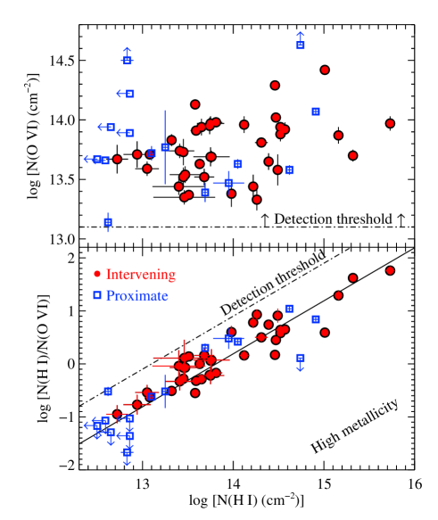
Figure 23.— Upper panel: The O VI vs. H I column densities for the O VI and H I components that have velocity centroids that agree within their $2\sigma$ uncertainties (see §2.3.2). Intervening systems are shown with filled circles and proximate absorbers are plotted with open squares with $1\sigma$ error bars. For several proximate absorbers, H I is not detected, and the plotted point marks the $3\sigma$ upper limit on $N$(H I). In two cases, the O VI is saturated, and $N$(O VI) is indicated as a lower limit. Lower panel: The log [H I/O VI] column density ratio vs. log $N$(H I) for the aligned components shown in the upper panel. The solid line shows the relation between $N$(H I)/$N$(O VI) and $N$(O VI) if $N$(O VI) is a constant equal to the median of the robust intervening sample (see Table 6). The solid line is plotted for illustration (see text) and is not a fit to the data. The dash-dot line shows the O VI detection threshold. In the lower panel, points in the upper-left region would have O VI column densities below our detection threshold, and points in the lower right would require high metallicities. Thus, the correlation of H I/O VI with $N$(H I) can be largely due to selection effects.

Finally, we consider the statistics of $N$(O VI) vs. $N$(H I) and the H I/O VI column density ratios in our O VI samples. These statistics can, in principle, provide insight about the physical conditions of the absorbers. However, because these absorbers can have a multiphase nature with contributions to $N$(H I) from low-ionization gas as well as high-ionization phases (see, e.g., §2.4.2; Chen & Prochaska 2000; Tripp et al. 2000; Richter et al. 2004; Sembach et al. 2004; Tumlinson et al. 2005; Savage et al. 2005), the H I/O VI ratio should be interpreted carefully. The H I in the PKS0312-770 absorber shown in Figures 2 and 3, for example, must include a substantial contribution from the low-ionization gas, and it is not at all clear how much of the H I is affiliated with the O VI-bearing gas. Comparison of the total H I and O VI column densities can introduce systematic errors because this can mix in some H I gas that is known to be unrelated to the O VI into the measurements. To overcome this problem, we strive to identify cases where the data indicate that the H I and O VI absorption lines are more likely to arise in the same gas. To achieve this, we focus in this section on the components which have well-aligned O VI and H I absorption components. As discussed in the previous section, Figure 20 shows that many of the O VI and H I profiles are well-aligned. This similarity is not necessarily expected in multiphase entities; different temperatures, turbulence, and/or bulk kinematics in the different phases would likely lead to detailed differences in the profiles in the low-ionization and high-ionization phases. The remarkable alignment of some of the components strongly suggests that in these cases, the O VI and H I are strongly mixed in a single gas phase, hence we concentrate on these aligned cases in this section. We note that there are other components with clear velocity offsets between the O VI and H I (see Figure 7); we discuss these more complicated cases in §4.2.

From our robust samples of intervening and proximate absorbers, we have selected all components whose O VI and H I velocity centroids are aligned to within their $2\sigma$ velocity-difference uncertainties. We employ these “well-matched” O VI + H I components for several purposes in the rest of this paper, and various measurements for the well-matched cases are plotted in Figures 23 - 36. Several useful properties of the well-aligned intervening components are listed in Table 7 including constraints on the plasma temperature and nonthermal broadening of the lines (see §4.1.1), measured H I/O VI and C III/O VI column-density ratios (including upper limits), and the classification (simple vs. complex) of the absorption system in which the particular component is found.

We show $N$(O VI) vs. $N$(H I) for the well-matched, robust sample in the upper frame of Figure 23. Applying a Spearman test to the intervening sample in Figure 23, we find that the probability of the null hypothesis (i.e., no correlation) is 2.7% . Thus, we find a weak indication that $N$(O VI) and $N$(H I) are correlated in the intervening absorbers. Interpretation of the proximate system data is complicated by the fact that H I is not detected at all in several proximate absorbers (see Figure 8), but Spearman tests nevertheless indicate that there is no significant evidence for any correlation of any combination of the proximate system H I and O VI column densities shown in the upper panel of Figure 23.

In the lower panel of Figure 23 we show the correlation between log [$N$(H I)/$N$(O VI)] and log $N$(H I) for the robust well-matched sample. Danforth & Shull (2005) have argued that this correlation is an important indicator of the multiphase nature of low$-z$ O VI systems and that the strong correlation of $N$(H I)/$N$(O VI) with $N$(H I) indicates that the O VI arises in collisionally ionized gas. We find from a Spearman test applied to the well-aligned sample in Figure 23 that the H I/O VI ratio is indeed highly correlated with H I, and we find that the slope in Figure 23 is fully consistent with the slope reported by Danforth & Shull (2005). However, this correlation is automatic at some level since H I/O VI is being correlated with $N$(H I). The solid line in Figure 23 shows the correlation that would result from a sample with a single (constant) O VI column density equal to the median $N$(O VI) that we measure from our robust intervening sample. The correlation in the lower panel of Figure 23 simply shows that $N$(O VI) is not strongly correlated with $N$(H I). Danforth & Shull (2005) argue that $N$(O VI) should be directly proportional to $N$(H I) if the gas is photoionized. While $N$(O VI) and $N$(H I) might be weakly correlated, Figure 23 clearly shows that $N$(O VI) is not linearly proportional to $N$(H I); there is substantial scatter in the data. However, the amount of O VI in an H I cloud depends on both the metallicity and the physical conditions of the gas, and it is not clear that $N$(O VI) should be strictly proportional to $N$(H I) in photoionized gas. We will return to this issue in §4.1.3, and we will show that the correlation in the lower panel of Figure 23 can arise naturally in photoionized gas.

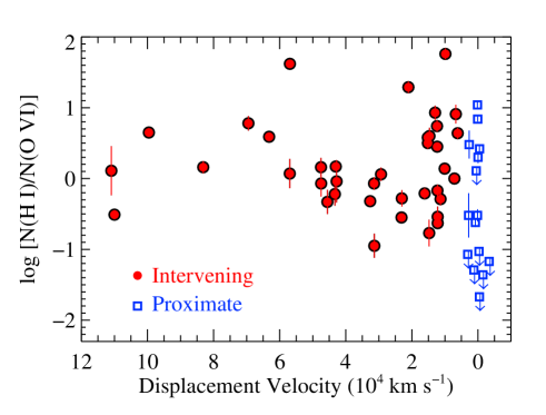
Figure 24.— The H I/O VI ratio vs. velocity of displacement from the QSO redshift. This figure uses the well-aligned component sample that is shown in Figure 23 with the same symbols. For clarity, some small artificial velocity offsets were applied to the clump of upper limits on the H I/O VI ratio for the proximate absorbers in the lower-right corner of the plot.

Also, there are some important selection effects that should be borne in mind when analyzing the lower panel of Figure 23. First, if the O VI column density is too low, the line will be lost in the noise. In our sample, we detect very few lines with log $N$(O VI) $<$13.1 (see Figure 18), and we take this as our O VI detection threshold. The dash-dot line in Figure 23 shows this detection threshold. We can see that this threshold explains the absence of points in the upper-left region of the lower panel of Figure 23; absorbers in that region would have undetectable O VI lines. We can detect absorbers that would populate the lower-right region of that plot, but any ionization mechanism would require a high metallicity to place points in that region. The lack of points in the lower right likely indicates that the O VI absorbers do not have such high metallicities.

We noted in §2.4.2 that there is a notable difference between the intervening and proximate absorbers: some of the proximate systems show no detectable, affiliated H I. Figure 23 shows that the majority of these H I-deficient proximate systems are located in a part of the $N$(O VI) - $N$(H I) parameter space where no intervening absorbers are found. More measurements of proximate absorbers are needed to determine if low H I/O VI ratios are a distinguishing signature of intrinsic absorbers, but the lack of analogous low H I/O VI components in the intervening absorbers suggests that there is very little contamination of the intervening sample with intrinsic absorbers that have been accelerated to high ejection velocities. Figure 24 shows the H I/O VI ratio of the matched intervening and proximate absorbers as a function of displacement velocity. We see that roughly one third of the of proximate systems have log [$N$(H I)/$N$(O VI)] $<-1$. If, for example, up to a third of the intervening systems are high-velocity ejected systems (as suggested by some papers, see §2.4.2), and one third of those ejected cases have log [$N$(H I)/$N$(O VI)] $<-1$, then we would expect to find $4-5$ absorbers in the intervening sample with similarly low H I/O VI ratios. This number of low H I/O VI systems is clearly not present in the matched intervening sample (see Figure 24). It remains possible that some of the intervening systems that are classified as multiphase absorbers because of substantial differences between the H I and O VI profile shapes are the high-velocity ejected systems, but at this juncture, we do not find any clear evidence that ejected, intrinsic absorbers are a significant source of contamination of the intervening O VI sample defined by $v_{\rm displ}>5000$ km s^-1.

4. Physical Conditions

Next we consider the physical conditions implied by our O VI and H I measurements. We first derive quantitative constraints on the gas temperatures in the components with well-matched O VI and H I components (§4.1.1), and then we discuss the implications of the well-aligned absorber properties regarding the process by which the gas is ionized (§§4.1.2, 4.1.3, 4.1.4). We will find that the simplest models favor an origin in cool, photoionized gas for a substantial fraction of the absorbers. However, in §4.2 we point out some of the complexities encountered in multiphase systems and the implications regarding hot gas in such absorbers, and we examine whether the broad Ly$\alpha$ components associated with hot O VI could be hidden in the noise (§4.2.1). In this section, we will focus primarily on the intervening absorbers, which are more pertinent to the primary goals of our survey, and we exclude the more uncertain measurements that are flagged with a colon in Table 3.

4.1. O VI Systems with Well-Aligned H I Components

4.1.1 Temperature Constraints

The line width of an individual absorption component provides a fundamental constraint on the temperature of the absorbing gas. If the line width is dominated by thermal motions, then the $b-$value is directly related to the gas temperature $T$ and the mass $m$ of the species,

$$T=\frac{mb^{2}}{2k}=A\left(\frac{b}{0.129}\right)^{2},$$ (7)

where $A$ is the atomic mass number and the numerical coefficient assumes that $b$ is in km s^-1 and $T$ is in K. In many situations, however, other factors will contribute to the line broadening such as turbulence or multiple unresolved components. If other factors are likely to contribute to the line broadening, then equation 7 can still provide a useful upper limit on $T$. However, if absorption lines from two or more species with significantly different masses are available (and are believed to arise in the same gas), then $b$ can be expresssed as a combination of a thermal broadening term and a nonthermal broadening term $b_{\rm nt}$,

$$b^{2}=(0.129)^{2}\frac{T}{A}+b_{\rm nt}^{2},$$ (8)

which can be solved for $T$ and $b_{\rm nt}$, assuming the nonthermal motions are adequately characterized by a Gaussian profile. This equation can provide valuable insights about the nature of the absorbers.

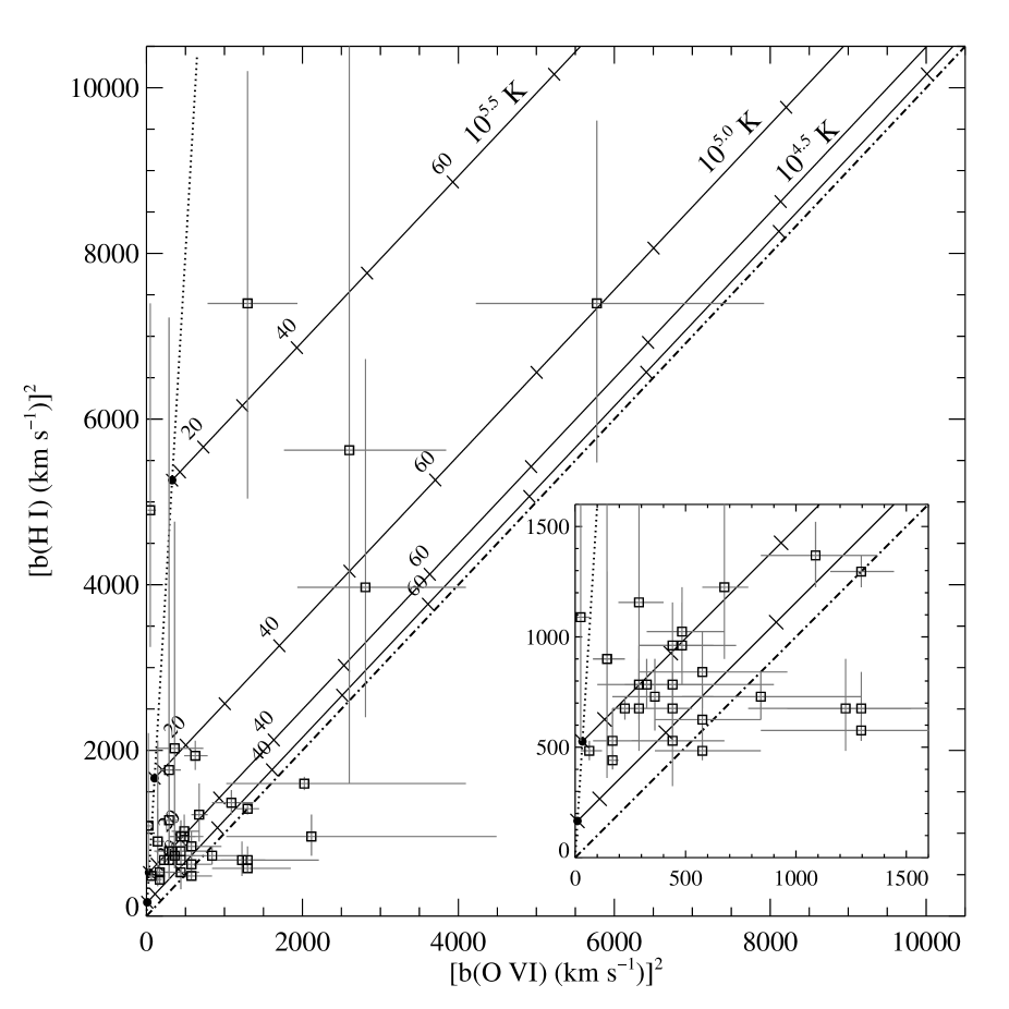
Figure 25.— Squared $b-$values of H I vs. O VI for the well-aligned components (§2.3.2). The measured points are shown by open squares with 1$\sigma$ error bars. For most of these aligned components, $b$(H I) $>\ b$(O VI), as expected if the H I and O VI are mixed together and arise in the same gas phase [the dash-dot line indicates the $b$(H I) = $b$(O VI) line of equality]. The dotted line shows the $b$(H I) = $4b$(O VI) locus; this is the relation for purely thermally broadened lines and represents the other boundary of physically possible measurements. Some of the cases that are outside of the physically-allowed region can be attributed to measurement errors, but we show in §4.2 that some of these cases could be due to multiphase media in which the O VI is close in velocity to narrow and broad H I components, and our algorithm has incorrectly assigned the O VI to the narrow H I line. The solid lines show loci of constant-temperature for log $T$ = 4.0, 4.5, 5.0, and 5.5 (from bottom to top, respectively), and the tick marks on each solid line indicate the values of $b_{\rm nt}$ that produce the $b$(H I), $b$(O VI) combination at the given temperature. The $b_{\rm nt}$ tick marks increase in increments of 10 km s^-1 from left to right. The $b_{\rm nt}=0$ km s^-2 points are indicated with a filled circle, and the $b_{\rm nt}$ = 20, 40, and 60 km s^-1 ticks are labeled on each constant-$T$ line. The dense cluster of measurements in the lower left indicates that the aligned components are relatively cold with $b_{\rm nt}\lesssim 30$ km s^-1. To show this cluster more clearly, the inset shows the same plot over a smaller $b^{2}$ range..

One of the main goals of this survey is to search for evidence of the shock-heated warm-hot intergalactic gas in order to understand the inventory of baryons in the universe (§1). In most theoretical studies, the WHIM is defined to have $T\geq 10^{5}$ K (but see Kang et al. 2005 for evidence that a substantial portion of the WHIM could be cooler). For O VI, $T\geq 10^{5}$ K implies that $b$(O VI) $\geq 10$ km s^-1. From Table 3 and Figure 18, we see that the majority of the intervening O VI absorption lines have sufficiently large $b-$values to be consistent with a WHIM origin. This is a necessary but insufficient requirement to establish that these absorbers originate in the WHIM, however, because if $b_{\rm nt}$ is substantial, $T\ll 10^{5}$ remains possible. Much more stringent constraints can be derived from H I, which has $b$(H I) $\geq$ 41 km s^-1 if $T\geq 10^{5}$ K.

Therefore, we next consider the temperatures implied by the well-matched sample of H I and O VI components that are well-aligned in velocity. The good correspondence of many of the aligned O VI and H I profiles (see Figs. 4 and 20) suggests that these O VI and H I lines arise in the same gas, and therefore we can employ the two versions of equation 8 for H I and O VI to solve for $T$ and $b_{\rm nt}$. Using the O VI and H I $b-$values for the aligned components and equations 7 and 8, we obtain the gas temperature constraints listed in Table 7. Columns 4 and 5 in Table 7 list the constraints implied from the O VI $b-$values only (eqn.7); column 4 gives the temperature implied by the best value of $b$(O VI) and column 5 lists the $3\sigma$ upper limit implied by the uncertainties in $b$(O VI). We treat these temperature constraints as upper limits because nonthermal broadening could be a significant source of line broadening. Columns 6 and 7 list the temperatures found by solving equation 8 with $b$(H I) and $b$(O VI); column 6 reports the best temperature and column 7 provides the $3\sigma$ upper limit found by propagating the $b-$value uncertainties through equation 8.

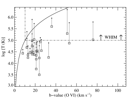
Figure 26.— Plasma temperatures implied by the H I and O VI $b-$values measured for well-aligned intervening components. Squares indicate the temperature implied by the best-fit O VI and H I $b-$values (solving eqn. 8), and the small dots connected to the squares by a vertical line show the $3\sigma$ upper limits on the temperature from propagation of the $b-$value uncertainties through eqn. 8. The solid line indicates the temperature implied by the O VI $b-$value if the line is predominantly thermally broadened (eqn. 7). The region above and to the right of the dash-dot line is consistent with the canonical WHIM temperature ($T\geq 10^{5}$ K).

Figure 27.— Distribution of temperatures determined for the aligned intervening O VI components in 0.2 dex bins. The temperatures were found by solving equation 8 with the measured H I and O VI $b-$values. The temperatures and amount of nonthermal broadening for individual components are summarized in Table 7. The open histogram indicates the total number of O VI components in a bin regardless of its classification; the hatched histogram shows the components in complex/multiphase systems only.

From equation 8, we see that at a constant temperature, the relationship between $b$(H I)² and $b$(O VI)² is a straight line with unity slope. Therefore, by plotting $b$(H I)² vs. $b$(O VI)², we can visually show where an H I + O VI absorber is located in ($T,b_{\rm nt}$) space. We show this visual representation of the $b-$values of the well-aligned absorbers in Figure 25. The advantage of this presentation is that the combinations of $T$ and $b_{\rm nt}$ can be quickly assessed by inspection. In addition, Figure 25 shows whether the lines are predominantly thermally broadened (or not) and whether the assertion that the H I and O VI are mixed together is physically reasonable. There are two physical limits on allowed $b$(H I), $b$(O VI) combinations if the H I and O VI are mixed together. The dash-dot line shows the physical limit of $b$(H I) = $b$(O VI); $b$(H I) $<b$(O VI) is unphysical but can arise from noise in the $b-$value measurements if the lines are mainly broadened by nonthermal motions and/or have large $b-$value uncertainties. The dotted line indicates the other physical limit, $b$(H I) = $4b$(O VI), which occurs if the lines are entirely thermally broadened. The solid lines are loci of constant temperature with log $T$ = 4.0, 4.5, 5.0, and 5.5 (from bottom to top, respectively). On each constant$-T$ locus, the tick marks indicate values of $b_{\rm nt}$ starting from $b_{\rm nt}$ = 0 km s^-1 and increasing in increments of 10 km s^-1 from left to right (the $b_{\rm nt}$ = 20, 40, and 60 km s^-1 ticks are labeled).

Several aspects of Figure 25 deserve comment. First, most of the well-aligned intervening components are not predominantly thermally broadened. Relatively few of the measurements are close to the $b$(H I) = $4b$(O VI) dotted-line locus expected for predominantly thermally broadened absorbers. Second, many of the points indicate temperatures well below the canonical 10⁵ K lower limit for WHIM plasma (see further comments below). Third, some points fall outside of the physically allowed regions. While some of these apparently unphysical combinations could be artifacts due to noise, we note that many of these cases have complex multicomponent structure, and this can lead to ambiguity in the assignment of O VI components with H I components. It remains possible that broad H I components are present in these absorbers, and the O VI has been inadvertently aligned with a narrow H I line that happens to have a similar velocity. We discuss this possibility in §4.2. In most of the aligned absorption lines, the H I $-$ O VI matching is clear and unambiguous (see examples shown in Figure 4), but a broad H I component could still be hidden in the noise (see §4.2.1).

Nevertheless, the simplest model is to assume that if the H I and O VI line centroids are well-aligned and the profiles have similar shapes, then the H I and O VI absorption lines arise in the same (single-phase) gas cloud. We adopt this assumption for the rest of this section. We plot the best temperatures and upper limits derived from $b$(H I) and $b$(O VI) (columns 6 and 7 from Table 7) as a function of $b$(O VI) in Figure 26, and we show the differential distributions of these estimations of $T_{\rm best}$ and $b_{\rm nt}$ in Figures 27 and 28, respectively. From these figures, we see that the quantitative results derived in this section corroborate the qualitative conclusion reached from comparison of the O VI and H I profiles in §3.4: a large fraction of the well-matched components appear to be too cold to arise in WHIM gas (with the standard $T>10^{5}$ K WHIM definition). Sixty-two percent of the $T_{\rm best}$ values in column 6 of Table 7 are below $10^{5}$ K. The $3\sigma$ upper limits provide more conservative constraints, but even the $T_{3\sigma}$ upper limits are inconsistent with WHIM temperatures for 44% of the aligned components. Evidently, many of the well-matched components are not consistent with collisional ionization at the standard temperatures where O VI is found in CIE, and most of these aligned components are not consistent with the standard temperatures expected for WHIM gas. It is possible that most of the WHIM gas is located in the multiphase absorbers (as we discuss below), but in the simple absorbers we find strong evidence that a substantial fraction of these systems are either photoionized or arise in collisionally ionized gas that is out of equilibrium.

It is interesting to examine the temperatures in Figures 26 and 27 more closely. While most of aligned components imply temperatures lower than log $T$ = 5.5, ten of the aligned components (26% ) in Table 7 imply log $T\geq$ 4.6, which is warmer than the temperatures expected in standard photoionization models (see, e.g., the photoionization models reported in Sembach et al. 2004 and Lehner et al. 2006). These moderately warm systems could arise in shock-heated gas that has cooled more rapidly than it can recombine and thus is in an overionized, moderately warm condition. It is also interesting to note that aligned components that are found within multiphase systems (indicated with hatching in Figures 27 and 28) tend to indicate higher temperatures and greater amounts of nonthermal broadening. Multiphase absorption could be more likely to occur in gas accreting into deeper potential wells because such locations are likely sites for shock heating but could also be places where more gas cools quickly due to processes such as thermal instability (e.g., Maller & Bullock 2004). Motivated by this possibility, we consider whether available non-equilibrium collisional ionization models agree with these observations in the next section (§4.1.2)

Figure 28.— Distribution of nonthermal broadening parameters (see equation 8) for the well-aligned intervening components in 5 km s^-1 bins (see Table 7). As in Figure 27, all of the aligned components from intervening systems are shown with an open histogram. The hatched histogram represents components from complex/multiphase systems only.

We have commented above on the fractions of the aligned components that are relatively cool. While we have not placed constraints on the temperatures of the non-aligned O VI components (i.e., those with significant velocity offsets between O VI and H I), we can nevertheless place a lower limit on the fraction of the O VI components that are relatively cold. There are 70 components in the robust intervening sample. From Table 7, we see that there are 24 components with log $T_{\rm best}<5.0$ in the simplest model. This indicates that at least 34% of the intervening components are cooler than the standard $10^{5}$ K WHIM cutoff. Conversely, at least 14% of the robust sample of intervening components has log $T_{\rm best}>4.6$ (hotter than expected in typical photoionization models).

4.1.2 Collisional Ionization Models

We have presented strong evidence that many of the low$-z$ O VI lines arise in cool gas. For many of the O VI components, the temperature constraints in Table 7 preclude a WHIM origin at the collisional ionization equilibrium temperatures where O VI is expected to peak in abundance (e.g., Sutherland & Dopita 1993). But could the absorption lines arise in collisionally ionized gas that is out of equilibrium?

In the context of the Milky Way ISM, the possibility that high ions could be detectable in non-equilibrium, overionized gas has long been considered (e.g., Kafatos 1973; Shapiro & Moore 1976; Edgar & Chevalier 1986; Indebetouw & Shull 2004; Gnat & Sternberg 2007). If shock-heated, highly ionized gas can cool more rapidly than it recombines, then species like O VI might be found in surprisingly cool material. ISM densities are substantially higher than IGM densities though, and in the context of the IGM, it is sometimes argued that this scenario is unlikely because the cooling timescale, $\tau_{\rm cool}=3kT/2n\Lambda(T)$, is quite long when the cooling function $\Lambda(T)$ for low-metallicity material (e.g., Sutherland & Dopita 1993; Gnat & Sternberg 2007) is combined with the theoretically expected low densities of IGM gas. If we use the parameters typically adopted for $\tau_{\rm cool}$ calculations (e.g., the gas is initially heated to $T>10^{6}$ K, $n<10^{-5}$ cm^-3, $Z<0.1Z_{\odot}$), we do find that it will not cool in a Hubble time (e.g., Dopita & Sutherland 2003; Shull et al. 2003). However, there are several factors that could make $\tau_{\rm cool}$ shorter: First, in low$-z$ IGM clouds where several metals are detected, studies have indicated metallicities significantly greater than 0.1 $Z_{\odot}$ (e.g., Savage et al. 2002; Jenkins et al. 2005; Tumlinson et al. 2005; Aracil et al. 2006; Lehner et al. 2006). Higher metallicity increases $\Lambda(T)$ (see Figure 4 in Gnat & Sternberg 2007) and thus decreases $\tau_{\rm cool}$. On the other hand, similar studies of low$-z$ systems with well-constrained metallicities have indicated $Z<0.1Z_{\odot}$ (e.g., Tripp et al. 2002,2005). There appears to be a very large range in the metallicity of the low$-$ IGM, and it is not clear what metallicity should be assumed for a random IGM cloud, but it has been shown that some clouds are significantly enriched and therefore could cool more quickly. Second, if the WHIM is heated by lower-velocity shocks, the initial temperature might be lower than usually assumed, which increases $\Lambda(T)$. If the initial temperature is only $10^{5.5}$ K, for example, the gas will cool more rapidly (see Figure 4 in Gnat & Sternberg). Thirdly, the gas densities could be somewhat higher than $10^{-5}$ cm^-3. For the well-aligned sample, log $N$(H I) ranges from $\approx$ 13.3 to 14.5 (see Figure 23). The H I number density $n$(H I) = $3.2\times 10^{-25}N$(H I)/$L$, where $L$ is the size of the cloud in Mpc. At log $T$ = 5.5, the H I ion fraction is $10^{-5.9}$ (Sutherland & Dopita 1993; Gnat & Sternberg 2007), so if $L$ = 100 kpc and $T=10^{5.5}$ K, the total H density in the well-aligned absorbers ranges from $\approx 5\times 10^{-5}$ cm^-3 to $\approx 8\times 10^{-5}$ cm^-3. The combination of higher densities, higher metallicities, and lower initial temperatures than usually assumed can lead to cooling times that are significantly shorter than the Hubble time.

The timescale to approach ionization equilibrium is approximately $\tau_{\rm ioneq}=[\tau_{\rm ion}^{-1}+\tau_{\rm rec}^{-1}]^{-1}$, where $\tau_{\rm rec}$ is the recombination time scale and the $\tau_{\rm ion}$ is the ionization timescale. Considering estimates of $\tau_{\rm ion}$ and $\tau_{\rm rec}$ for O VI, O VII, and O VIII at WHIM temperatures and densities (see, e.g., Figure 3 in Yoshikawa & Sasaki 2006), we see that $\tau_{\rm ioneq}\ll\tau_{\rm Hubble}$, and for many combinations of IGM physical conditions, $\tau_{\rm ioneq}<\tau_{\rm cool}$. Therefore CIE could be a good approximation for O VI, O VII, and O VIII in WHIM absorbers.

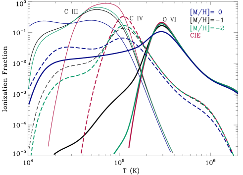
Figure 29.— Comparison of nonequilibrium ion fractions in isochoric radiatively cooling gas for O VI (thick solid lines), C IV (dashed lines), and C III (thin solid lines) calculated by Gnat & Sternberg (2007) for logarithmic metallicities of [M/H] = 0 (blue curves), [M/H] = $-1$ (black curves), and [M/H] = $-2$ (green curves). The collisional ionization equilibrium (CIE) ion fractions are also shown with red lines.

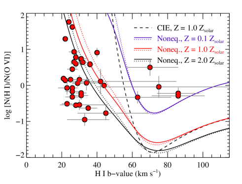
Figure 30.— Observed H I/O VI ratios vs. H I $b-$values measured in the intervening absorber components that are aligned to within their 2$\sigma$ component centroid uncertainties (filled circles; these are the same data presented in Figure 23 but only for the intervening systems). The observations are compared to predictions from the ionization models of Gnat & Sternberg (2007) for collisional ionization equilibrium (CIE, dashed line) and for nonequilibrium, radiatively cooling models for gas with $Z=0.1Z_{\odot}$ (purple lines), $Z=1.0Z_{\odot}$ (red lines), and $Z=2.0Z_{\odot}$ (black lines). For each metallicity, the solid lines show the results for gas cooling isochorically (constant density), and the dotted lines show the isobaric (constant pressure) models. The models fail to explain the majority of the observed measurements. The models predict ion fractions as a function of gas temperature; we have converted the model temperatures to $b-$values assuming pure thermal broadening of the lines. If non-thermal motions contribute to the line broadening, the discrepancy between the models and the observations is even worse.

Since these absorbers could be cooling rapidly, we will now consider whether the observed properties of the O VI systems could be consistent with predictions from radiatively cooling, overionized gas models. For this purpose, we list in columns 9 and 10 of Table 7 two observables that can be readily compared to nonequilibrium model predictions: the $N$(H I)/$N$(O VI) and $N$(C III)/$N$(O VI) column density ratios measured in the well-matched components of intervening absorbers. In many of our systems, C III is not detected, so we provide $3\sigma$ limits based on the measured upper limit on the C III rest-frame equivalent width assuming the linear portion of the curve of growth applies. In some cases, C III is detected but is strong enough so that it could be underestimated due to saturation (see, e.g., Savage et al. 2002); in these cases we treat the measured $N$(C III) as a lower limit.

Gnat & Sternberg (2007) have recently modeled nonequilibrium radiatively cooling gas, and they provide predictions for these column density ratios as a function of gas temperature. They have modeled both isochoric and isobaric cooling gas, and they provide predictions for models with a wide range of metallicities. In Figure 29, we compare the ion fractions of C III, C IV, and O VI predicted by Gnat & Sternberg (2007), for isochoric radiatively cooling gas, to the ion fractions for these species from CIE. This figure demonstrates several important aspects of nonequilibrium radiatively cooling models when applied to extragalactic O VI absorbers. First, nonequilibrium ionization effects depend on the metallicity of the gas and become increasingly important as the metallicity increases. This is expected from the timescale arguments: the cooling rate depends on metallicity, so when the metallicity is low, $\tau_{\rm ioneq}<\tau_{\rm cool}$ and CIE is a good approximation. However, the metallicity at which nonequilibrium effects set in depends on the species. For example, if the overall metallcity [M/H] = $-2$, then the nonequilibrium O VI ion fraction is almost identical to the equilibrium ion fraction (compare the thick green and red lines in Figure 29). In comparison, nonequilibrium effects are already significant for C III and C IV at [M/H] = $-2$. Even at [M/H] = $-1$, the nonequilibrium O VI ion fraction is quite low at log $T<$ 5. From Figure 29, it appears the nonequilibrium effects will lead to detectable O VI in cool gas only if the metallicity is relatively high. Nevertheless, we inevitably must compare O VI with other species to discriminate bewteen various ionization models, so nonequilbrium effects on other species can affect conclusions about O VI systems.

Figure 30 shows the observed H I/O VI ratios vs. the measured H I $b-$values for the well-matched components (filled circles). These measurements are compared to the predicted ratios from the Gnat & Sternberg (2007) isochoric models (solid lines) and isobaric models (dotted lines) for the three metallicities. For reference, the dashed line plots the CIE ratio from Gnat & Sternberg (2007). Gnat & Sternberg predict these ratios as a function of temperature $T$; we have converted their temperatures to the corresponding $b-$value that H I would have at that $T$ for a purely thermally broadened line. We see from Figure 30 that none of these models agree with the bulk of the matched components. In general, at the temperature implied by the narrowness of the observed H I lines, the models predict H I/O VI ratios that are too high. A fraction of the matched absorbers are consistent with the model predictions, but only if the metallicity is relatively high.

The Gnat & Sternberg (2007) models have even greater difficulty with the measured C III/O VI ratios and limits. Figure 31 compares the observed C III/O VI ratios and limits to the predictions from the isochoric models of Gnat & Sternberg (2007). In this figure we have retained the temperatures from the model and we have plotted the measured ratios vs. the observed temperatures and limits from Table 7. For the majority of the matched intervening components, the models predict C III/O VI ratios that are one to several orders of magnitude too high. The isobaric models are not shown in Figure 31, but these models predict even higher C III/O VI ratios and thus fit the observed data even more poorly.

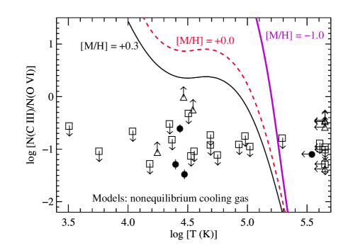
Figure 31.— Comparison of the observed $N$(C III)/$N$(O VI) ratios for the well-aligned components of intervening systems (as in Figure 23) to the predictions for this ratio from the nonequilibrium ionization models of Gnat & Sternberg (2007). The temperatures for the observed components are the best values derived from the O VI and H I $b-$values as described in §4.1.1; absorbers without temperature constraints are shown at far right. This figure only shows intervening systems: squares indicate cases where C III is not detected and the ratios are derived from the $3\sigma$ upper limits on $N$(C III), triangles indicate lower limits in cases where C III could be underestimated due to line saturation, and filled circles indicate cases with good C III measurements. The solid curves show the model predictions for isochoric nonequilibrium cooling gas for logarithmic metallicities [M/H] = $-1.0$ (purple line), 0.0 (red line), and 0.3 (black line) from Gnat & Sternberg (2007). The isobaric Gnat & Sternberg (2007) models fit the observations even more poorly than the isochoric models.

We conclude that the Gnat & Sternberg (2007) nonequilibrium models usually fail the match the observed column-density ratios in the well-aligned O VI absorbers. One caveat, however, is that Gnat & Sternberg (2007) neglect photoionization in their calculations. Given the low densities expected for IGM absorbers (see above), photoionization is likely to be important. The combination of nonequilibrium collisional ionization plus additional photoionization from impinging UV light could bring the models into better agreement with the observations because photoionization could significantly reduce the H I and C III columns without reducing $N$(O VI) much, especially if the ionizing radiation is predominantly from stars (which do not emit many photons with sufficient energy to ionize O V into O VI). Of course, how photoionization affects species like C III depends on the physical conditions of the gas. If the ionization parameter is low, photoionization could boost $N$(C III) thereby leading to greater discrepancy with the observations. New nonequilibrium models that include photoionization would be valuable. We will show in §4.1.4 that simple models that include both photoionization and collisional ionization can satisfy the observational constraints, but realistic modeling of time-dependent effects is beyond the scope of this paper.

4.1.3 Photoionization Models

Is collisional ionization required at all in the intervening absorbers? Are the absorber properties consistent with the expected characteristics of purely photoionized gas? We have evaluated the viability of pure photoionization as the ionization mechanism using the photoionization code CLOUDY (v96.01, Ferland et al. 1998). We treat the absorbers as plane-parallel slabs photoionized by a background UV radiation field with a specified shape and intensity. Apart from the shape and intensity of the ionizing flux, the absorber model properties depend primarily on the ionization parameter $U$ of the gas ($U\equiv n_{\gamma}/n_{\rm H}$ = ionizing photon density/total particle density), the metallicity, and the total hydrogen column density. We assume that background QSOs and AGNs provide the bulk of the ionizing flux, and we use the Haardt & Madau (1996) QSO background but with the modifications provided by Haardt (2006) [for motivation of the UV background update, see Madau et al. 1999; Haardt & Madau 2001; Shull et al. 1999; Scott et al. 2004].

Usually, photoionization models are constrained by requiring the models to fit the measured column densities of multiple detected metals such as Si III, C III, and C IV (in addition to O VI and H I). With measurements from multiple species, both the metallicity and the ionization parameter can be constrained by models (e.g., Tripp et al. 2002; Savage et al. 2002; Lehner et al. 2006). Unfortunately, in the majority of our intervening O VI systems, we only detect O VI and H I (and occasionally C III). Nevertheless, we can certainly check to see if the photoionization model predictions are consistent with the measurements. In §4.1.2, we showed that the Gnat & Sternberg (2007) nonequilibrium collisional ionization models are clearly not consistent with the observations; will we find a similar result from photoionization models?

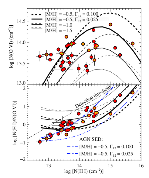
Figure 32.— Observed O VI and H I column densities for matched components in intervening systems (filled circles); the multicolor points represent components from complex/multiphase absorbers. As in Figure 23, the upper panel shows log $N$(O VI) vs. log $N$(H I), and the lower panel plots log [$N$(H I)/$N$(O VI)] vs. log $N$(H I). These observations are compared to the predicted column densities from six photoionization models that assume that the gas density ($n_{\rm H}$) and the H I column density are related by equation 9 (see Schaye 2001) and that the gas is photoionized by the UV background light from QSOs/AGNs (Haardt & Madau 1996; Haardt 2006). The solid lines represent models that assume that the H I photoionization rate $\Gamma_{12}=0.025$ (see text), and dashed lines assume $\Gamma_{12}=0.100$. For each assumed value of $\Gamma_{12}$, models are shown with overall metallicities of [M/H] = $-1.5$ (thinnest lines), [M/H] = $-1.0$ (thicker lines), and [M/H] = $-0.5$ (thickest lines). In the lower panel an additional two photoionization models that assume ionization by an AGN-dominated spectral energy distribution (using the shape from Mathews & Ferland 1987) are also compared to the data (triple-dot-dash lines) for two values of $\Gamma_{12}$.

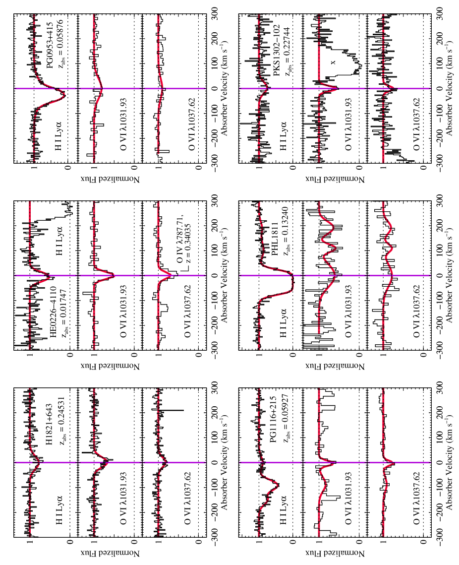
Figure 33.— Six of the seven O VI absorbers with the lowest H I/O VI ratios in individual components (the seventh case with a low H I/O VI ratio is shown in Figure 37). Each panel shows the H I Ly$\alpha$ and O VI $\lambda\lambda$1031.93,1037.62 absorption profiles with sight line and absorber redshift indicated in the Ly$\alpha$ panel. At least one (but not necessarily all) of the components has a low H I/O VI ratio (see Table 3).

The ionization parameter depends on the gas density and the ionizing radiation density. To estimate the gas density, we can invoke the arguments presented by Schaye (2001), who showed that if an intergalactic H I cloud is photoionized and in hydrostatic equilibrium, then the characteristic size of the absorber will be the Jeans length, and the total hydrogen number density $n_{\rm H}$ can be directly estimated from the H I column density:

$$n_{\rm H}\approx 10^{-5}\left[\frac{N({\rm H~{}I})}{2.3\times 10^{13}}\right]^{2/3}T_{4}^{0.17}\Gamma_{12}^{2/3}\left(\frac{f_{g}}{0.16}\right)^{-1/3},$$ (9)

where we have rearranged Schaye’s equation 8 and $T_{4}=T({\rm K})/10^{4}$, $\Gamma$ is the hydrogen photoionization rate, $\Gamma_{12}=\Gamma({\rm s^{-1}})/1\times 10^{-12}$, and $f_{g}$ is the fraction of the total mass contributed by the baryonic gas. Within a reasonable range for gas temperatures of photoionized gas, the model predictions are not overly sensitive to $T$; we assume $T$ = 20,000 K for our calculations. We also assume that $f_{g}$ is close to the “universal” value (i.e., $\Omega_{b}/\Omega_{m}$), and following Schaye (2001) we use $f_{g}$ = 0.16. While Schaye (2001) derived equation 9 analytically, very similar results for photoionized gas have emerged from hydrodynamic simulations of the IGM (see, e.g. equation 7 in Davé et al. 1999), and the relationship between overdensity and H I column in the simulations has been discussed in many papers. We will use the results from Schaye (2001) in the rest of this paper, but tests show that we would reach similar conclusions if we used the relationship from the simulations instead.

The hydrogen photoionization rate depends on the shape and intensity of the UV background. The best observational constraints on the UV background intensity at $z\approx$ 0 come from the observations of Weymann et al. (2001). Based on deep upper limits on H$\alpha$ emission from the H I 1225+01 intergalactic cloud (Giovanelli & Haynes 1989), Weymann et al. derive upper limits on the intensity of the UV background at 1 Rydberg, $J_{\nu}$(1 Ryd). Their upper limit depends on the geometry of the cloud, and they derive limits ranging from $J_{\nu}$(1 Ryd) $<0.96\times 10^{-23}$ to $<3.84\times 10^{-23}$ ergs cm^-2 s^-1 Hz^-1 str^-1. For the UV background from QSOs, these intensity limits imply photoionization rates ranging from $\Gamma_{12}\approx 0.025$ to $\Gamma_{12}\approx 0.10$. These limits are in good agreement with constraints obtained from other techniques (see §5 in Davé & Tripp 2001). We will use these two values for $\Gamma_{12}$ to investigate the viability of photoionization models applied to low$-z$ O VI systems. One appealing aspect of applying the Schaye arguments to photoionization models is that this ensures that the absorber size is a physically reasonable size – the absorber size is that which results from hydrostatic equilibrium. Using Schaye’s equation 12, we find that the absorber sizes are $\lesssim$ 750 kpc (450 kpc) for log $N$(H I) $>$ 13.0 and $\Gamma_{12}=0.025\ (0.100)$. The corresponding Hubble width due to Hubble broadening is $b_{\rm H}\approx H(z)L/2\lesssim 28\ (17)$ km s^-1. This amount of Hubble broadening is quite reasonable compared to the nonthermal broadening estimated for the aligned absorbers (see Table 7).

Using equation 9 to specify the gas density and using the modified Haardt & Madau (1996) UV background from QSOs, Figure 32 compares the predicted O VI and H I column densities from several photoionization models to the observed column densities from the matched intervening sample (Table 7). In this figure, solid lines indicate models that assume $\Gamma_{12}$ = 0.025, and dashed lines show models that adopt $\Gamma_{12}$ = 0.100. For each of these $\Gamma$ values, the thin, thicker, and thickest lines represent models with logarithmic metallicities [M/H] = $-1.5,-1.0,$ and $-0.5$, respectively. In the lower panel of Figure 32, we also show the H I/O VI ratio from models that are photoionized by an AGN spectral energy distribution (SED, triple-dot-dash lines), using the Mathews & Ferland (1987) characterization of the shape of an AGN SED, with $\Gamma_{12}$ = 0.025 and 0.100. The AGN SED model is provided to illustrate the effect of changing the shape of the ionizing flux field.

We have already noted that there is evidence of substantial metallicity variations in the IGM. It is also likely that the shape as well as the intensity of the ionizing UV background varies significantly in the IGM. Regions that are closer to AGNs/QSOs could naturally be exposed to a radiation field that is brighter but also has a different shape. The contribution from stellar flux escaping from galaxies is uncertain but could also lead to ionizing radiation shape and intensity variations. Finally, the particle density can vary from place to place, which changes the ionization parameter in photoionization models. Figure 32 shows that changes in these variables can lead to significant variations in the H I/O VI ratio even in simple photoionized models. We see that when the O VI detection threshold is factored in, photoionization models for H I clouds in hydrostatic equilibrium can easily explain the observed O VI and H I properties of many of the low$-z$ O VI absorbers. The models can produce the observed column densities, and moreover, the weak correlation of $N$(O VI) with $N$(H I) is a natural result of these models (as long as the UV background and IGM metallicity are variable in the low-z Universe).

The points with the lowest H I/O VI ratios in Figure 32 are not expected in the models photoionized by the Haardt & Madau (1996) UV background unless the metallicity is quite high. However, these points can be explained by models that have a similar metallicity to the rest of the sample but are photoionized by an AGN-like SED (such models are shown with the triple-dot-dash lines in the lower panel of Figure 32), i.e., a harder radiation field. One might wonder if these low H I/O VI ratios could be measurement artifacts, so we show the absorption profiles for these cases in Figure 33. From this figure, we 4 out of 7 of the lowest-ratio cases are in systems with simple component structure, and the lines are securely detected. Therefore, most of the low ratios are not simply due to measurement errors. It would be interesting to test whether the low-ratio absorbers are found in closer proximity to a source of harder ionizing flux. We do see that the intervening systems with the lowest H I/O VI ratios are close to the ratios seen in the low-$N$(H I) proximate absorbers (see Figure 23). The proximate absorbers are close (in redshift) to the background QSO, so these cases are likely to be ionized by a radiation field with an AGN SED shape. The similarity of the proximate absorbers to the low-ratio intervening systems is consistent with the conclusion that a nearby AGN could be dominating the radiation field in all of these cases.

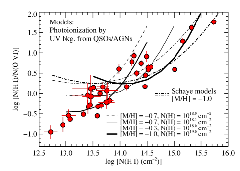
Figure 34.— Comparison of the observed H I/O VI ratios in components of intervening systems (filled circles) to the H I/O VI ratios predicted by generic photoionization models (solid and dashed lines). The models assume photoionization by the UV background from quasars and AGNs according to the calculations of Haardt & Madau (1996). The variable parameters in the models shown are the metallicity, [M/H], the total (H I + H II) hydrogen column density $N$(H), and the ionization parameter. The [M/H] and $N$(H) assumed for each curve are indicated in the legend. Lower ionization parameters produce higher H I/O VI ratios. For comparison, the photoionization models that result from invoking Schaye’s arguments (i.e., using equation 9) with [M/H] = $-1.0$ are shown with dash-dot lines; the thick dash-dot line assumes $\Gamma_{12}=0.100$, and the thin dash-dot line assumes $\Gamma_{12}=$ 0.025.

It is interesting to see that the physical framework of Schaye (2001) naturally explains the observed O VI and H I properties of the well-aligned components, but we note that more generic photoionization models that do not invoke equation 9 are also successful. We show several more generic photoionization models in Figure 34. In these models we have again assumed the modified Haardt & Madau (1996) UV background, but we have selected various values of $N_{\rm total}$(H) and [M/H] without requiring $n_{\rm H}$ and $N$(H I) to be related by equation 9. For a given model, the ionization parameter decreases along the model curve from left to right in Figure 34. For purposes of illustration, in this figure we show $N$(H I)/$N$(O VI) vs. $N$(H I) and we replot the two Schaye-based models from Figure 32 with [M/H] = $-1.0$ and $\Gamma_{12}$ = 0.025,0.100. The generic photoionization models can also reproduce the observed O VI and H I column densities with reasonable values for $N_{\rm total}$(H) and [M/H]. We do note that both the Schaye-based models and the generic models require relatively high metallicities ($Z\gtrsim 0.3Z_{\odot}$) for some of the O VI systems, which might be somewhat surprising. However, similar metallicities have been indicated by studies of comparable absorbers with detections of multiple metals (e.g., Savage et al. 2002; Aracil et al. 2006; Lehner et al. 2006).

Evidently, purely photoionized gas can produce the observed O VI and H I column densities. However, we can see from Figures 32 and 34 that there are substantial degeneracies in the photoionization models when the only observational constraints are from O VI and H I, and it would be very helpful to include constraints from other metals in the ionization analysis. Moreover, we found in §4.1.2 that the nonequilibrium collisional ionization models were able to match some of the H I/O VI ratios but were much harder pressed to fit the C III/O VI constraints. For both of these reasons, we now examine whether our photoionization models are consistent with the observed C III/O VI constraints from Table 7. In Figure 35 we compare the C III/O VI constraints to the predictions from the Schaye-based and generic photoionization models. In this plot, the model C III/O VI ratios are not dependent on metallicity because $N$(C III) and $N$(O VI) change homologously with metallicity. Figure 35 shows that the photoionization models are consistent with the constraints provided by the current observations for a large fraction of the well-aligned components. The generic photoionization models are consistent with all of the measurements provided that the total hydrogen column (H I + H II) ranges from $10^{17}$ up to $\gtrsim 10^{19}$ cm^-2. We do notice that the models that employ equation 9 with $\Gamma_{12}=0.025$ or 0.100 appear to be most consistent with the higher $N$(H I) systems, and the Schaye-based models do not fit the four cases that provide the best C III measurements. Since most of the matched intervening O VI systems only provide upper limits on $N$(C III), the data remain consistent with the Schaye-based models for most of the measurements, but more sensitive measurements of (or upper limits on) the C III column densities would provide a useful test of the Schaye-based photoionization predictions (as shown in §5.1.2, future C IV measurements would be similarly useful for testing these models). The Schaye models move toward better agreement with those points if $\Gamma_{12}$ is reduced. Since the best observational constraints still provide only upper limits on $\Gamma_{12}$, this solution remains a possibility, but it appears that $\Gamma_{12}$ must be reduced by a large amount. The Schaye-based models can also be moved closer to the well-measured C III/O VI ratios by using a UV background radiation field that includes a greater contribution from stellar flux escaping from galaxies, but this would upset the agreement with the H I/O VI models. The discrepancy with the best C III measurements in Figure 35 could be a symptom of a serious problem with this model. This could indicate that the clouds are not in hydrostatic equilibrium, for example, or that multiphase models are required even for the apparently simple cases. Future studies should revisit the Schaye-based models with a larger sample of more-sensitive C III and/or C IV measurements.

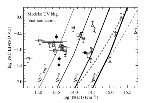
Figure 35.— Comparison of the observed C III/O VI ratios vs. log $N$(H I) in components of intervening systems (with symbols coded as in Figure 31) to the C III/O VI ratios as a function of log $N$(H I) predicted by generic photoionization models (solid lines). The photoionization models assume the Haardt & Madau (1996) UV background from QSOs/AGNs. Four model curves are shown corresponding to total (H I + H II) hydrogen columns of log $N$(H) = 17.5, 18.0, 18.5, and 19.0; each model is shown with a solid curve labeled with its total H column [the line thickness increases with $N$(H)]. The predicted C III/O VI ratios depend primarily on the ionization parameter; increasing the ionization parameter decreases the C III/O VI column density ratio. Changing the overall metallicity of the model does not move the curves in this plot because $N$(O VI) and $N$(C III) increase (or decrease) homologously with increasing (or decreasing) metallicity. The gray dashed lines represent the photoionization models that result from the model of Schaye(2001) with $\Gamma_{12}=$ 0.025 (thick dashed line) or $\Gamma_{12}=0.100$ (thin dashed line).

Figure 36.— Comparison of the observed H I/O VI ratios (upper panel) and the observed C III/O VI ratios (lower panel) to four “hybrid” ionization models that include both collisional ionization and photoionization. Both panels show the same ionization models, and the symbols have the same meaning as in Figure 31. Three of the models assume $Z=0.1Z_{\odot}$ ([M/H] = -1.0) with ionization parameters fixed at log $U=-1.63$ (thick solid line), log $U=-1.38$ (thin solid line), and log $U=-1.13$ (dashed line). The dash-dot line assumes $Z=1.0Z_{\odot}$ and log $U=-1.38$. Changing the overall metallicity affects the H I/O VI ratio but does not change the C III/O VI ratio. The parameters of the models in this plot were chosen for purposes of illustration; these are not fits to the data.

4.1.4 Hybrid Models (Collisional and Photoionization)

We have shown that if the aligned O VI and H I lines are cospatial, then the available models in which the gas is predominantly collisionally ionized to do not agree with the observed properties of the O VI absorbers (§4.1.2). Predominantly photoionized models can explain most of the measurements but often require a relatively high metallicity (§4.1.3). However, the best temperatures implied by the line widths (§4.1.1), while too cool to produce O VI in collisional ionization equilibrium, are sometimes higher than the temperatures expected in predominantly photoionized gas. This raises the question of whether photoionization and collisional ionization are both important in these absorbers.

We can provide a simplified evaluation of whether “hybrid” ionization models (i.e., including important contributions from collisional and photoionization) are plausible using CLOUDY. By running CLOUDY with the plasma temperature locked at a specified input value and including photoionization from the UV background, we can assess the effects of the combined ionization mechanisms. Such models solve for ionization equilibrium but are not in thermal equilbrium (heating does not balance cooling). In Figure 36 we show CLOUDY models at various fixed temperatures (shown on the x-axis) and photoionized by the Haardt & Madau (1996) QSO background flux. The models are compared to the observed H I/O VI and C III/O VI column-density ratios of the aligned components from Table 7. These calculations have three adjustable parameters: the temperature, metallicity, and ionization parameter. The curves show models with [M/H] = $-1$ and [M/H] = 0 ($Z=0.1Z_{\odot}$ and $1.0Z_{\odot}$) and three values for the ionization parameter. Our intention here is not to fit the ratios but to assess whether or not the models are plausible. We see that with reasonable values for the temperature and ionization parameter, these hybrid models can achieve good agreement with the observed ratios. In some cases, the models and measurements agree with [M/H] = $-1.0$. However, in the small number of cases where good C III measurements are available, close inspection shows that high metallicities are required in these hybrid models as well. Changing the overall metallicity does not change the C III/O VI ratio because both C III and O VI change by the same amount. However, the H I/O VI ratio is inversely proportional to the metallicity. We thus see from Figure 36 that in some cases, a better overall fit to the O VI, C III, and H I columns can be obtained with higher metallicities. As we discuss in §5, in the future it will important to obtain good measurements of multiple metal species in order to constrain the ionization and metallicity of as many specific systems as possible.

4.2. Physical Conditions in Complex Multiphase O VI Systems

Evidently, many of the well-aligned systems show compelling indications of cool gas ($T<10^{5}$ K), and among currently available models, these cool absorbers are best explained as photoionized gas. Is there any observational evidence of the WHIM in the nearby universe then? X-ray absorption lines (e.g., the O VII K$\alpha$ transition) are potentially useful for finding WHIM gas because the X-ray absorbers persist in hotter plasmas. X-ray spectroscopy has been used to search for the WHIM, and while some redshifted X-ray absorption lines have been reported (e.g., Fang et al. 2002; Mathur et al. 2003; Nicastro et al. 2005), the reliability of the detections has been debated (Kaastra et al. 2006; Rasmussen et al. 2002,2007; Bregman 2007; but see also Fang et al. 2007; Williams et al. 2007). X-ray absorption lines have been robustly detected at $z_{\rm abs}\approx 0$ (e.g., Nicastro et al. 2002; Fang et al. 2006), but there is evidence that the $z_{\rm abs}\approx 0$ X-ray absorbers arise in gas clouds that are relatively close to the Milky Way (Futamoto et al. 2004; Wang et al. 2005; Fang et al. 2006), perhaps even within a few kpc of the Milky Way disk (Yao & Wang 2005), and thus are more likely to be hot Galactic ISM gas than WHIM clouds.

In the ultraviolet bandpass, the strongest evidence of WHIM-temperature plasma is the 3.9$\sigma$ detection of Ne VIII reported by Savage et al. (2005) in the strong O VI absorber at $z_{\rm abs}$ = 0.20701 toward HE0226-4110. In this case, the Ne VIII column cannot be produced in plausible photoionization models, and the Ne VIII/O VI ratio requires $T=5.4\times 10^{5}$ K in collisional ionization equilibrium. It is interesting to note that this absorber is a complex case with multiple components in the H I profiles and low-ion metals that trace cooler (probably photoionized) phases of the absorption system. Other multiphase, multicomponent O VI absorbers have similarly been argued to have characteristics of warm-hot collisionally ionized gas (e.g., Chen & Prochaska 2000; Tripp et al. 2000; Prochaska et al. 2004; Shull et al. 2003; Tumlinson et al. 2005). The fact that all of these systems that present evidence of hot gas are multiphase absorbers raises a question: is the warm-hot gas primarily located in the complex multiphase absorbers? This is a crucial question for the inventory of baryons in the low$-z$ IGM (see §5.1.1). We have classified roughly half of the intervening sample as multiphase absorbers (§2.4.2). Because they are intrinsically complex, multiphase O VI systems often require detailed analyses (e.g., Tripp et al. 2001; Richter et al. 2004; Sembach et al. 2004; Savage et al. 2005; Tumlinson et al. 2005). Complete analysis of the full sample of multiphase absorbers is beyond the goals of this paper. However, it is useful to present a few examples of how the WHIM can be difficult to identify in multiphase absorbers.

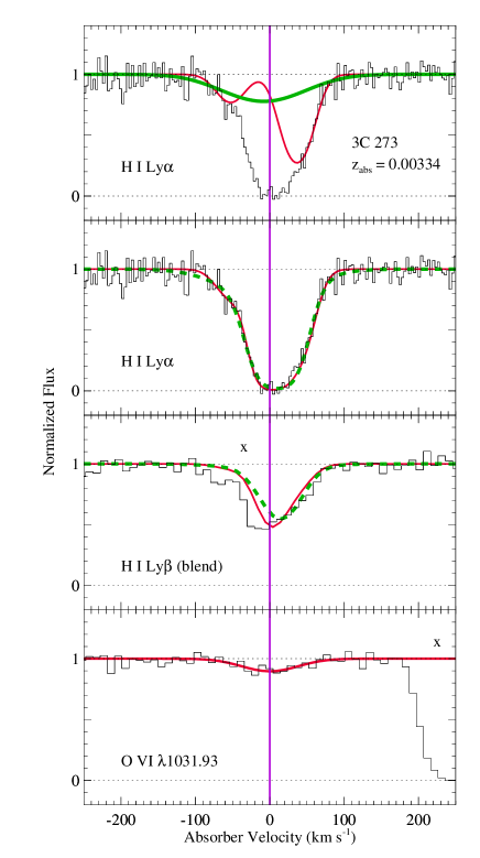
Figure 37.— Comparison of two comparably good fits to the H I Ly$\alpha$ and Ly$\beta$ profiles of the O VI absorber at $z_{\rm abs}$ = 0.00334 in the spectrum of 3C 273.0. In the second and third panels, the thin red line shows the three-component fit, and the thick dashed green line shows an alternative fit that uses only two components (the bottom panel shows the O VI $\lambda$1031.93 line, which is fitted with a single component). The top panel shows the difference between the alternative fits to the H I profiles: the three-component fit uses two narrow components (shown with a thin-red line) to fit the inflections in the wings of the Ly$\alpha$ profile, but the two component fit employs a single broad feature (shown with a thick green line) to fit these features. The H I Ly$\beta$ profile is partially affected by a blend with Milky Way H₂ absorption (see Sembach et al. 2001). Xs mark unrelated absorption.

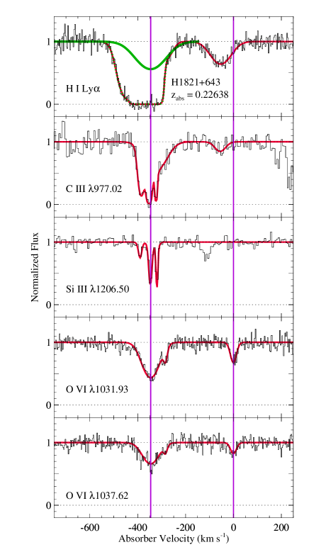
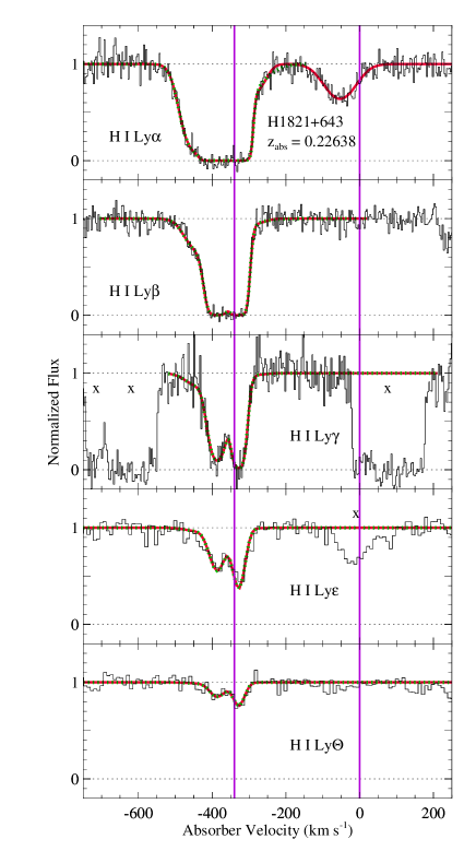
Figure 38.— Selected absorption profiles (histograms) of the complex, multiphase O VI absorbers at $z_{\rm abs}$ = 0.22496 and 0.22638 in the spectrum of H1821+643 (plotted in the $z_{\rm abs}$ = 0.22638 frame). Voigt-profile fits are overplotted with smooth lines in each panel, and the vertical lines indicate the $v=0$ km s^-1 points for $z_{\rm abs}$ = 0.22496 and 0.22638 (i.e., the centroids of the O VI absorbers). As discussed in the text, several aspects of these absorbers suggest the presence of hot gas. The H I panels show a comparison of two comparably good fits to the H I Lyman series lines in the complex, multiphase O VI absorber at $z_{\rm abs}$ = 0.22496. The red line shows the fit reported in Table 3, and the dotted green line shows an alternative H I fit with the velocity centroid of one H I component locked to the centroid of the O VI lines. The column density and $b-$value of the H I component with the locked velocity centroid are freely varied in the alternative fit (only the centroid is locked). The locked component in the final fit is shown with a thick green line in the top-left panel. Unrelated absorption lines are denoted with Xs.

One problem with multiphase absorbers arises from limitations of Voigt-profile fitting when dealing with complex component structure (§2.3). In moderate S/N data, the appropriate number of components to fit to a multicomponent profile can be ambiguous, and this can have a substantial impact on the results for some of the components. Figure 37 shows the $z_{\rm abs}$ = 0.00334 absorber toward 3C 273.0, which provides an example of this problem. In this case, the Ly$\alpha$ profile clearly shows a significant but blended absorption feature at $v\approx-50$ km s^-1. This feature cannot be caused by the main H I component at $v=0$ km s^-1 and this motivates a fit with at least two components. However, the positive-velocity side of the Ly$\alpha$ profile is also asymmetric with a “ledge” of pixels at $v\approx 35$ km s^-1 (most easily seen in the upper panel of Figure 37). This asymmetry suggests the presence of a third component. But in these data, systematic noise could be the origin of the ledge feature. The second and third panels in Figure 37 compare the results from a two-component fit (dashed green line) to the three-component fit (thin red line). The two-component fit provides a somewhat better reduced $\chi_{\nu}^{2}$ = 1.15 (compared to $\chi_{\nu}^{2}$ = 1.33 for the three-component model) and thus was favored in Table 3. However, the improvement in $\chi_{\nu}^{2}$ mainly results from a better fit to the Ly$\beta$ profile, which is confused by blending with Galactic H₂ absorption, and the two models fit the Ly$\alpha$ profile comparably well. The main H I component does not change much in the two- vs. three-component fit, but as shown in the top panel of Figure 37, the properties of the weaker component(s) are dramatically different in the two fits. The two-component fit requires a very broad H I component that is aligned with the O VI absorption within the $1\sigma$ centroid uncertainties. The three-component fit, on the other hand, results in three narrow H I lines (the main component plus the two weaker components shown with a red line in the top panel of Figure 37), and while the O VI is still aligned with the main component, in this case $b$(O VI) $\gg b$(H I), which is unphysical. The O VI $\lambda$1031.93 line is detected at the 4.5$\sigma$ level in the FUSE spectrum of 3C 273.0, but the line is broad and shallow. It is possible that the O VI profile is composed of three components that align with three H I components, but we cannot discern the O VI components at the available resolution and S/N ratio. Thus, this system is difficult to interpret. To overcome these fitting problems requires excellent data with high spectral resolution and high S/N.

This problem with identification of broad Ly$\alpha$ components in multiphase systems is exacerbated by high H I column densities. Consider the strong O VI absorber at $z_{\rm abs}$ = 0.20266 toward PKS0312-770 (shown in Figures 2 and 3). In this absorber, one or more of the components have $N$(H I) $\gtrsim 10^{17}$ cm^-2, which produces a “boxcar” Ly$\alpha$ absorption profile with a black core over a large velocity range (see the upper left panel of Figure 2). In this case, if there is a broad and relatively shallow H I component that arises in the O VI-bearing gas, it would likely be impossible to detect. Such a component would have miniscule optical depth in higher Lyman series lines and thus would be undetectable at available S/N levels, and in the Ly$\alpha$ profile, it would be hidden in the black core of the boxcar profile.

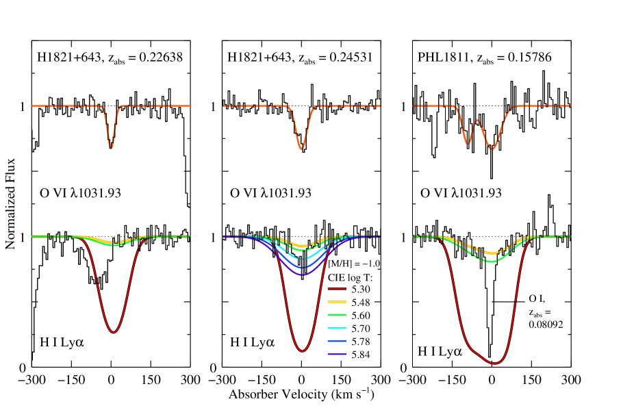
Figure 39.— Examples of the comparison of predicted H I Ly$\alpha$ lines, assuming the O VI arises in equilibrium collisionally ionized gas with $Z=0.1Z_{\odot}$, to the observed Ly$\alpha$ absorption profiles. The left and middle panels show the H1821+643 absorption systems at $z_{\rm abs}$ = 0.22638 and 0.24531, respectively, and the right panel shows the PHL1811 system at $z_{\rm abs}$ = 0.15786. In each panel, the upper histogram indicates the continuum-normalized O VI $\lambda$1031.93 profile and the lower histogram is the Ly$\alpha$ line. Note that the PHL1811 Ly$\alpha$ line at $z_{\rm abs}$ = 0.15786 is blended with O I $\lambda$1302.17 absorption from the Lyman-limit absorber at $z_{\rm abs}$ = 0.08092 discussed by Jenkins et al. (2005); the narrow core is due to the O I line. The smooth curve overplotted on the O VI line is the Voigt-profile fit from Table 3. Using the O VI column density from the Voigt-profile fit, we have determined the corresponding column density and $b-$value that the H I would have if it were in CIE with $Z=0.1Z_{\odot}$ and log $T$ = 5.30, 5.48, 5.60, 5.70, 5.78, and 5.84. The predicted Ly$\alpha$ profiles for the different assumed temperatures are represented by different line shades as indicated in the key in the middle panel. For purposes of discussion, we show the models for all of these temperatures in the middle panel, but we only plot the models with log $T$ = 5.30, 5.48, and 5.60 in the left and right panels. In this figure, the data have been binned to 7 km s^-1 pixels in order to better reveal any weak structure in the wings of the profiles.

And, there is some evidence that broad shallow Ly$\alpha$ components could be present in the the high$-N$(H I), multiphase absorbers. Figure 38 presents an example. This figure shows the H1821+643 O VI absorbers at $z_{\rm abs}$ = 0.22496 and 0.22638 (plotted in the $z_{\rm abs}$ = 0.22638 frame). Focusing first on the $z_{\rm abs}$ = 0.22497 system, we see that this is a multiphase metal system that is similar to the PKS0312-770 absorber shown in Figure 2. Comparing the C III, Si III, and O VI lines, we see that the C III and Si III profiles show three narrow components that are well-aligned. In contrast, the O VI profiles are smoother and clearly have different component structure. These profile differences are not due to thermal broadening and different species masses because carbon and oxygen have similar masses. Rather, these differences are due to multiple phases in this absorber. Now, turning to the H I Lyman series lines, we see that the two main, high$-N$(H I) components are well-constrained by the higher series lines. However, our original H I fit (in Table 3) did not result in any broad Ly$\alpha$ components, nor did it indicate any components that are aligned with the centroid of the O VI absorption. Following our usual procedure, the original fit allowed all component parameters ($v,b,$ and $N$) to freely vary during the fitting process. Interestingly, if we lock the velocity centroid of only one of the components to equal the centroid of the strongest O VI component (and we allow all the other parameters to vary freely), we obtain a comparably good fit. However, the locked component results in a broad Ly$\alpha$ component with $b$(H I) = 81${}^{+13}_{-11}$ km s^-1 and log $N$(H I) = 13.80$\pm$0.09 at the O VI velocity. The two fits to the H I lines are shown in Figure 38 with a red line and a dotted green line, and the broad Ly$\alpha$ line resulting from the locked$-v$ fit is indicated with a thick green line in the upper-left panel of Figure 38. We can see that the two fits are nearly indistinguishable, and the fits have nearly identical goodness of fit ($\chi_{\nu}^{2}$ = 1.030 vs. $\chi_{\nu}^{2}$ = 1.031). Between the two fits, the main two components (i.e., the two components evident in the higher Lyman series) change by tiny amounts; the changes occur in the weaker components required to fit the structure in the wings of the Ly$\alpha$ and $\beta$ profiles. However, these changes in the weak outlying components have major implications for the gas conditions. If we use the H I $b-$value from the locked fit together with the main-component O VI $b-$value, these measurements imply that the temperature of the O VI -bearing gas is log $T$ = 5.47. Assuming the H I and O VI ion fractions from collisional ionization equilibrium at this temperature, the measured column densities would then imply an oxygen abundance of [O/H] = $-1.4$.

These examples show that broad H I components could be present in the complex profiles, and in some cases, the combination of broad H I and O VI is consistent with WHIM temperatures and relatively low metallicities. These results are intriguing, but we must recognize that this only shows that hot gas is allowed by the data; these analyses do not uniquely require the presence of WHIM material. Without additional information, it can be difficult to discriminate between the fits shown in these examples. As noted, high S/N and spectral resolution would be helpful for constraining the physical conditions in these absorbers. Also, ancillary species such as Ne VIII can be immensely valuable for identification of hot gas (e.g., Savage et al. 2005). X-ray absorption lines would also be useful, but the spectral resolution available in the X-ray bandpass is still quite limited.

4.2.1 Hidden Broad H I Components?

Figure 38 demonstrates another notable characteristic of multiphase absorbers. We have remarked above that multiphase systems have larger velocity offsets between the H I and O VI centroids (see Figure 7). The $z_{\rm abs}$ = 0.22638 absorber in Figure 38 shows an example of one of the largest velocity offsets between H I and O VI in an intervening absorber: in this system, the O VI is detected $v=0$ km s^-1 while H I and weak C III are found at $v=-54$ km s^-1. Some H I absorption is present in the velocity range where O VI is detected, but this could be just the wing of the H I line at $-54$ km s^-1. Why does this well-detected O VI absorber have so little affiliated H I? One possibility is that this absorber is similar to the proximate absorbers and has a very high metallicity so that the affiliated H I column is too low to be detected.

However, another possibility is that this particular O VI doublet arises in collisionally ionized hot plasma with a temperature that makes the H I difficult to detect. The measured O VI $b-$value is $16\pm 2$ km s^-1, which is consistent with gas at $T\approx 10^{5.5}$. The left panel of Figure 39 shows theoretical H I Ly$\alpha$ profiles that would be expected to be affiliated with this O VI absorber in collisionally ionized gas at log $T$ = 5.30, 5.48, and 5.60 with $Z=0.1Z_{\odot}$. These predicted H I profiles use the Gnat & Sternberg (2007) CIE ion fractions to predict the H I column density (based on the measured $N$(O VI) and assumed metallicity), and the line widths are for the purely thermally broadened case (nonthermal broadening can only make the H I lines broader). We see that with log $T$ = 5.30, a strong (and easily detected) H I line is expected (red line in Figure 39). The H I line is strong because even though the H I ion fraction is low at this $T$, the O VI ion fraction drops very rapidly at log $T<5.5$ (see Figure 29), and consequently, $N$(H I) has to be high in order to produce the observed $N$(O VI). Of course, $N$(O VI) can be increased by increasing $Z$ and/or $N$(H I); an alternative solution is that $Z\gg 0.1Z_{\odot}$. However, we see from Figure 39 that if log $T$ = 5.48 or 5.60, close to the temperature of peak O VI abundance in CIE, then the affiliated $N$(H I) is low enough so that the expected Ly$\alpha$ profile (yellow or green lines in Figure 39) would be difficult or impossible to detect at the current S/N levels. Thus, this system could be in the warm-hot range with a realistic metallicity, and the expected broad H I would be hidden in the noise.

This raises a question: could similar “hidden” broad components be present in the aligned components discussed in §4.1.1? The middle panel of Figure 39 explores this possibility. This panel shows the well-aligned H I and O VI absorption lines at $z_{\rm abs}$ = 0.24531 in the spectrum of H1821+643 with theoretical Ly$\alpha$ profiles, calculated as described in the previous paragraph, for log $T$ = 5.30, 5.48, 5.60, 5.70, 5.78, and 5.84. We see that none of these model Ly$\alpha$ profiles fit the observed Ly$\alpha$ line very well. However, if this is a multiphase absorber with a narrow core from a lower-ionization phase that does not contribute to the O VI absorption, then a broad component would be allowed by the data as long as the temperature is in a narrow range (or $Z\gg 0.1Z_{\odot}$). We see that as above, warm-hot gas with log $T\approx 5.30$ or less is ruled out. Likewise, models with log $T\gtrsim$ 5.6 are ruled out; these models lead to Ly$\alpha$ profiles that are too strong and too broad. We conclude that this aligned O VI $-$ H I absorber could harbor a hidden broad Ly$\alpha$ component arising in the hot O VI phase, but only if the absorber is multiphase and the temperature is fine-tuned to a relatively narrow range near the O VI peak temperature and/or the metallicity is relatively high.

We noted in §4.1.1 that some of the aligned absorbers are outside of the physically allowed range of $b$(H I) and $b$(O VI). Occasionally, these unphysical cases could be due to coincidental alignment with unrelated absorption lines. The right panel of Figure 39 shows an example of coincidental alignment with unrelated absorption in the O VI absorber at $z_{\rm abs}$ = 0.15786 toward PHL1811. In this case, an apparently very narrow H I line seems to be aligned with the strongest component of a multicomponent O VI profile, and the candidate H I line is too narrow (compared to O VI) to be in the physically allowed regime. This unphysical combination is due to coincidental alignment of the O VI with an unrelated line: the narrow component in this case is actually not H I but rather is the O I $\lambda$1302.17 line from the Lyman limit absorber at $z_{\rm abs}$ = 0.08092 (see Jenkins et al. 2005). However, close inpection of the profile reveals weak absorption in the wings of the narrow O I feature. Those weak absorption wings do not appear to be due to O I because that component structure is not corroborated by stronger metal-line profiles of other low ions at the O I redshift. The weak components could be due to H I Ly$\alpha$ absorption at the O VI redshift. Interestingly, if the two O VI components at $z_{\rm abs}$ = 0.15786 have log $T$ = 5.48 and $Z\approx 0.1Z_{\odot}$, then the two expected broad Ly$\alpha$ components associated with the O VI would explain the weak components in the wings of the O I profile (see the yellow line in Figure 39).

Hidden broad Ly$\alpha$ lines are allowed for most of the intervening O VI absorbers. As shown in columns 4 and 5 of Table 7, the O VI line widths usually allow temperatures near the O VI peak (log $T\approx$ 5.5), and given the typical $N$(O VI), at this temperature an affiliated broad Ly$\alpha$ component would usually be hidden in the noise. This explanation requires that essentially all of the intervening O VI absorbers are multiphase because another (O VI-free) phase is required to explain the rest of the Ly$\alpha$ absorption. For many of the absorbers, the temperature or metallicity must be tuned to avoid producing overly strong broad Ly$\alpha$. However, some of the strong multiphase systems have broad features that could be due to O VI at somewhat lower temperatures (e.g., Tripp et al. 2001). This scenario is similar to the favored models for the O VI HVCs seen in the vicinity of the Milky Way (Sembach et al. 2003).

4.2.2 O VI in Interface Layers?

The correlation of log [$N$(H I)/$N$(O VI)] with log $N$(H I) could be an indication that the O VI absorption arises in some type of interface layer on the surface of a lower-ionization H I cloud. In this argument, the O VI column density is determined by the interface physics and is independent of the H I column density of the interior cloud. This scenario is not required by the data: we have shown in Figure 32 and §4.1.3 that photoionization models can explain the correlation if the IGM metallicity and UV background shape and intensity are variable. However, we have also shown in the previous section that the current data cannot rule out hidden broad Ly$\alpha$ lines that would indicate that the O VI arises in a hot phase that is closely aligned in velocity with a cooler lower-ionization phase that produces the bulk of the detected H I absorption.

To evaluate this hypothesis, it is useful to consider FUSE observations of O VI absorption detected in the very local interstellar medium (LISM) within a few hundred parsecs of the Sun (Oegerle et al. 2005; Savage & Lehner 2006). In these samples, the short pathlength to the background star ($d\leq$ 230 pc) precludes production of O VI by photoionization. In addition, the Sun is surrounded by a bubble of hot, X-ray emitting gas with $T\approx 10^{6}$ K (e.g., Smith et al. 2007), so this context provides observational information on the properties of O VI absorption arising in interface layers.

Interestingly, Savage & Lehner (2006) find that find $\approx$40% of the O VI absorption line velocity centroids in the LISM are aligned with C II absorption centroids to within $\pm$ 10 km s^-1 (see their Figure 11). This supports the hypothesis that O VI could originate in an interface without having different kinematics (velocity centroids) compared to the low-ionization phase. However, Savage & Lehner also find that more than half of their local O VI lines show clear and significant velocity offsets. Overall, the velocity offsets of the LISM O VI absorbers appear to be similar to those observed in the extragalactic O VI systems of this paper. However, there is a significant difference between LISM O VI absorbers and the extragalactic systems: the LISM O VI column densities are substantially lower. Savage & Lehner find 12.38 $\leq$log $N$(O VI) $\leq$ 13.60 in the LISM with a median of log $N$(O VI) = 13.10. These observed LISM columns are comparable to the $N$(O VI) values theoretically predicted to be found in conductive interfaces between cool clouds and hot gas (e.g., Slavin 1989; Borkowski et al. 1990), but the extragalactic $N$(O VI) measurements are up to $\approx$50 times higher. Therefore, many interfaces are required to explain the QSO O VI systems according to these interface models and LISM observations. This problem is exacerbated by the fact that the extragalactic absorbers are likely to have significantly lower metallicities than the LISM systems; lower metallicity will further reduce the $N$(O VI) expected in an interface. With the requirement of many interfaces to produce the observed $N$(O VI), we would expect to find complexity in the absorption profiles (due to variations of the H I/O VI ratios and H I vs. O VI kinematics from one cloud to the next within the multilayer system). Some of the QSO O VI profiles show considerable complexity, but others appear to be relatively simple. Given this problem, it is not clear if interface models can fit the properties of the simple extragalactic systems.

However, we note that other models of interstellar O VI production (see Table 1 in Indebetouw & Shull 2004), such as radiatively cooling clouds or bubbles blown by supernovae/stellar winds, do predict O VI columns that are substantially higher. We also note that in a survey of 148 Milky Way stars, Bowen et al. (2007) find that the scatter in $N$(O VI) does not decrease with increasing sight line pathlength, which indicates that the O VI absorption lines do not arise in clouds with a fixed size and density. These factors suggest that collisionally ionized hot O VI can originate in a variety of contexts with significant variations in cloud characteristics. The Milky Way O VI HVCs (Sembach et al. 2003; Wakker et al. 2003) suffer a similar problem to the extragalactic systems: the O VI in Galactic HVCs is thought to arise in interfaces (e.g., Sembach et al. 2003; Ganguly et al. 2005), but the observed HVC O VI columns tend to be substantially greater than the expected $N$(O VI) in interfaces. We conclude that the interface physics may not yet be sufficiently well-understood or is oversimplified in available models. While there are some significant discrepancies, the interface hypothesis for the origin for extragalactic O VI absorbers is viable and deserves further study.

5. Discussion and Future Observations

5.1. Intervening Absorbers

5.1.1 Baryonic Content and Missing Baryons

What do these analyses imply about the baryonic content of the low$-z$ IGM and the missing baryons? Several previous papers have shown that low-redshift O VI absorbers harbor roughly 5% of the baryons in the nearby Universe (Tripp et al. 2000,2006b; Savage et al. 2002; Sembach et al. 2004; Danforth & Shull 2005; Lehner et al. 2006). Most of these papers have assumed that the mean metallicity of the O VI systems is $Z_{\rm O~{}VI}=0.1Z_{\odot}$ and that the O VI ion fraction ($f_{\rm O~{}VI}=$ O VI/O_total) is less than $\approx 0.2$. The latter assumption is secure (see, e.g., the Appendix in Tripp & Savage 2000), but as noted by Lehner et al. (2006) and as discussed above, many recent studies have found $Z>0.1Z_{\odot}$ in nearby IGM absorbers. The absorber baryonic content $\Omega_{\rm b}$(O VI) $\propto Z_{\rm O~{}VI}^{-1}f_{\rm O~{}VI}^{-1}$, so increased metallicity decreases the baryonic content by the same factor. The uncertain metallicity of the absorbers is currently a large source of uncertainty in $\Omega_{\rm b}$(O VI). New measurements of $\Omega_{\rm b}$(O VI) should employ detailed metallicity constraints for each absorber in the sample instead of assuming a mean $Z_{\rm O~{}VI}$, or at least the assumed value for $Z_{\rm O~{}VI}$ should be based on a sample of measured metallicities. Unfortunately, many of the O VI systems are only detected in O VI and H I. With only these two species, the metallicity of the systems remains uncertain. Better constraints on $\Omega_{\rm b}$(O VI) will require secure measurements of other metals in the O VI absorbers.

However, another problem with $\Omega_{\rm b}$(O VI) estimates is that most previous studies have included all intervening O VI absorption systems in the $\Omega_{\rm b}$(O VI) measurement regardless of the physical conditions of the absorbers. The contribution to the baryon budget from low$-z$ photoionized gas has been separately estimated from studies of Ly$\alpha$ lines (e.g., Penton et al. 2004; Lehner et al. 2007) and is often included in baryon inventories (e.g., Fukugita et al. 1998), so by including photoionized and collisionally ionized O VI systems together in a single estimate of $\Omega_{\rm b}$(O VI), some double-counting of baryons could occur. To avoid this double counting, $\Omega_{\rm b-Total}$(O VI) should be split into $\Omega_{\rm b-WHIM}$(O VI) and $\Omega_{\rm b-Photo}$(O VI), the baryonic content of WHIM and photoionized O VI systems. Our physical conditions analysis indicates that at least 34% of the intervening O VI components present compelling evidence of cool temperatures (log $T<$ 5.0). However, we also found in §4.1.1 that at least 14% of the O VI components have log $T>4.6$, which is hotter than the temperatures typically expected in photoionized intergalactic gas.

The intermediate-temperature cases with log $T>$ 4.6 could arise in plasma that was initially shock-heated and is now rapidly radiatively cooling. Shock-heated gas with $T<10^{5}$ K is predicted by some theoretical models, so these intermediate-temperature O VI systems could be WHIM material. Kang et al. (2005) report that in their hydrodynamic models of cosmological structure growth, many sheet-like structures are shock-heated and contain material that conceptually should be classified as “WHIM” plasma, but in their models, the shock velocities are lower, and they conclude that an important fraction of the baryons are in the shocked IGM but with $T<10^{5}$ K, which they refer to as the “low-temperature” WHIM. Kang et al. (2005) analyze the physical conditions and ionization of the low-temperature WHIM, and they find that this IGM phase is predominantly photoionized. Moreover, they note that $\approx 60$% of the O VI absorbers originate in the low-temperature, photoionized WHIM in their simulations. The models of Kang et al. (2005) are consistent with the observational constraints that we have derived in this paper.

We have also noted that the O VI absorbers that provide the strongest evidence of $T>10^{5}$ K plasma tend to be complex, multiphase absorbers with multiple H I components (some of which do not have associated O VI) and (in some cases) clear absorption by low ionization stages. In these multicomponent, multiphase systems, it is easy to hide a broad H I component that would be associated with hot O VI. We classify 53% of the intervening systems as complex/multiphase absorbers, and these complex systems could be the primary harbor of the $T>10^{5}$ K plasma. In fact, some of the simulations show that $T>10^{5}$ K plasma is often surrounded by cooler gas, and these simulations predict these “embedded” WHIM locations produce peaks in O VI density maps (see, e.g., Figures 4-6 in Cen & Ostriker 2006). It seems likely that random sight lines through the cosmological simulations would often find that the WHIM is located in regions where cooler gas phases are also present, and consequently O VI from these regions will be affiliated with complex, multicomponent H I and lower-ion profiles at similar velocities, like some of the observed multiphase O VI systems. Theoretical predictions regarding the characteristics of O VI and H I profiles in various environments would be helpful for checking the consistency of the models and the observations.

It should also be borne in mind that the detectability of O VI depends on the metallicity of the gas. If the missing baryons are predominantly located in gas that is shock-heated when it first accretes into galaxy potentials, then the WHIM plasma could have a relatively low metallicity, and O VI could be difficult to detect in the WHIM phase in currently available data. Instead of O VI, broad H I Ly$\alpha$ lines (BLAs) can be used to search for the low$-z$ WHIM, and several studies have reported detections of BLA candidates at low redshifts (Tripp et al. 2001; Bowen et al. 2002; Richter et al. 2004,2006a,b; Sembach et al. 2004; Lehner et al. 2007). Only a small fraction of the reported BLAs are also detected in O VI (the O VI doublet is covered but not detected in most cases). We can show that the lack of affiliated O VI absorption is consistent with a WHIM origin for the BLAs. The approximate carbon metallicity of the high-redshift IGM is [C/H] $\lesssim-2.5$ (Schaye et al. 2003). If the low-redshift WHIM has a similar metallicity, then using the O VI and H I ion fractions from Gnat & Sternberg (2007), we find that $N$(O VI)/$N$(H I) $\lesssim 0.25$. Since most low$-z$ BLAs have $N$(H I) $\lesssim 10^{14}$ cm^-2 (Lehner et al. 2007), in collisionally ionized plasma we predict that the corresponding $N$(O VI) $\lesssim 10^{13.4}$ cm^-2, which is comparable to the lowest O VI columns that we are currently able to reliably detect. Since the WHIM metallicity could be substantially lower than $-2.5$, and because $N$(O VI)/$N$(H I) $\lesssim 0.25$ is derived at the peak of the O VI/H I vs. temperature curve, the O VI/H I ratios could be substantially lower in BLAs. Thus, it may not be surprising that O VI is not usually detected in the BLAs. In a recent study of the low$-z$ H I lines detected in STIS echelle spectra, Lehner et al. (2007) estimate that at least $\approx 20$% of baryons could be found in broad Ly$\alpha$ absorbers.

5.1.2 Future Studies of Intervening Absorbers

Several future observations would be valuable for gaining insight about the low$-z$ IGM. First, it will be important to obtain high signal-to-noise spectra. In addition to revealing weaker O VI and ancillary metal lines, higher S/N ratios will help to establish whether the BLAs are truly single-component, smooth and broad Gaussian features. Current data often suggest that H I lines are BLAs, but due to modest S/N, it remains possible that these BLA candidates are actually unrecognized blends of several adjacent components (see, e.g., Richter et al. 2006b). With higher S/N, it will often be possible to recognize profile asymmetries that reflect multiple, blended components. High S/N is also crucial for probing the presence of hidden broad Ly$\alpha$ components that could be associated with collisionally ionized O VI (§4.2.1). Second, it will be useful to detect other species, including O III, O IV, and O V as well as ions of other elements, to enable more constrained modeling of the ionization and metallicity of the absorbers. We have discussed the utility of C III in this regard. The Ne VIII $\lambda\lambda$770.41, 780.32 doublet is an important doublet for future studies since it probes plasma with $T\approx 6\times 10^{5}$ K (Savage et al. 2005), but with the HST bandpass, this will only be accessible in intermediate-redshift absorbers ($z_{\rm abs}\gtrsim$ 0.50). The C IV $\lambda\lambda$1548.21, 1550.78 doublet will be an important metal to search for in many O VI systems. Figure 40 shows the C IV/O VI ratios predicted by the various photoionization models considered in §4.1.3. From this figure, we see that the C IV/O VI ratio is usually significantly greater than the corresponding C III/O VI ratio in photoionized O VI systems. The N V $\lambda\lambda$1238.82, 1242.80 doublet is also useful and has been occasionally detected (e.g., Savage et al. 2002; Tumlinson et al. 2005). The N V doublet is weaker and more difficult to detect, but this can be overcome with high S/N observations. A greater difficulty with nitrogen is that it can be underabundant due to nucleosynthesis effects in low-metallicity gas (e.g., Henry et al. 2000), which can cause confusion in ionization models. Bearing such effects in mind, with measurement of two or more metals as well as H I, it will be possible to place specific, precise constraints on the physical conditions and metal enrichment of the low$-z$ IGM.

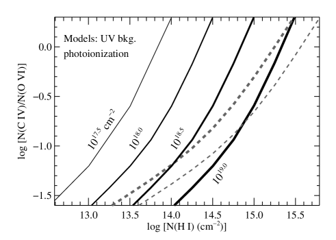
Figure 40.— Predicted C IV/O VI vs. $N$(H I) from the same photoionization models presented in Figure 35 with the same line codes.

More detailed comparisons between the observations and theoretical predictions from cosmological simulations would also be instructive. The Kang et al. simulations predict that a large fraction of the low$-z$ O VI absorbers should arise in relatively cool gas, but it should be noted that other simulations have also indicated that some fraction of the O VI absorption occurs in predominantly photoionized gas (e.g., Cen et al. 2001; Fang & Bryan 2001; Chen et al. 2003). In the simulations, how do the O VI and H I profiles compare in photoionized regions? Conversely, what are the characteristics of the O VI and H I profiles in the warm-hot, shocked regions in the simulations? For example, is the WHIM expected to be typically found in close proximity to cooler gas thereby resulting in complex, multiphase profiles? Another question is whether the similarity of many of the observed O VI and H I profiles could arise in multiphase gas in which the O VI traces a hotter phase and the H I arises in cooler gas. A wind-blown bubble-like feature might have hot O VI in an interface just inside the bubble edge and cool H I around the outer periphery; could this configuration result in well-matched O VI and H I profiles? Intuitively, differences in factors such as temperature and turbulence in the hot vs. the cold gas would be expected to impart different kinematic characteristics to the O VI and H I in this situation. Detailed assessments of the O VI and H I characteristics in theoretical simulations would provide valuable insight for interpreation of the O VI absorbers.

5.2. Proximate Absorbers

5.2.1 Evidence of AGN Feedback?

One of the goals of our survey is to search for evidence of feedback from outflows driven by QSOs/AGNs (see §1). Some papers have argued that a significant fraction of QSO absorption lines with $v_{\rm displ}>5000$ km s^-1 are actually intrinsic QSO absorption systems that have been ejected by the QSO/AGN and accelerated to dramatic outflow velocities (§2.4.2). One of the QSOs in our sample (3C 351.0) does reveal a complex, multicomponent O VI system with 13 O VI components spread over $\approx 2800$ km s^-1 at $z_{\rm abs}\approx z_{\rm QSO}$ (Yuan et al. 2002). This complex proximate absorber, which does show evidence of partial covering of the QSO continuum and broad emission line sources (see Yuan et al.), is probably best described as a mini-BAL. Apart from this particular system, we do not find any evidence of high-speed QSO outflows in our sample. We do see some clear differences between O VI absorbers at $v_{\rm displ}<5000$ km s^-1 and those at $v_{\rm displ}\gg 5000$ km s^-1: (1) $dN/dz$ for O VI increases substantially as $z_{\rm abs}$ approaches $z_{\rm QSO}$, (2) we find a marginal indication, based on the proximate absorber $b-$value distribution, that proximate O VI lines tend to be narrower than the intervening O VI lines, and (3) $\approx$40 % of the proximate O VI systems have much lower H I/O VI ratios than the intervening systems.

The lower H I/O VI ratios in proximate systems could be due to ionization effects (due to proximity to the bright backgound QSO), higher metallicity, or both. Figure 41 shows the predicted $N$(O VI) from photoionized models with log $N$(H I) = 13.0, [M/H] = $-1.0$, and two different ionizing radiation fields, the Mathews & Ferland (1987) approximate description of an AGN spectral energy distribution and the Haardt & Madau (1996) UV background that we have used previously. We see that the Mathews & Ferland AGN SED does increase the amount of O VI predicted from a low-$N$(H I) cloud compared to the UV background expected in the intervening IGM. However, we also show the measured $N$(O VI) that we find in eight proximate absorber components that have log $N$(H I) $\lesssim$ 13.0, and we see that even the Mathews & Ferland model falls short of the observed columns, in some cases by more than an order of magnitude. Realizing that most of the eight cases in Figure 41 provide only upper limits on $N$(H I), and realizing that the ionization parameter does not necessarily have the value that maximizes the predicted $N$(O VI), we conclude that these proximate absorbers require metallicities that are much greater than 0.1 $Z_{\odot}$.

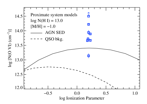
Figure 41.— Photoionization models with low H I column densities and moderately low metallicities for two ionizing radiation fields: the approximate description of the spectral energy distribution of an AGN from Mathews & Ferland (1987) [solid line] and the QSO background from Haardt & Madau (2006) [dashed line]. These models have a fixed H I column density (log $N$(H I) = 13.0) and metallicity ($Z=0.1Z_{\odot}$), and with these parameters, the predicted O VI column is shown as a function of the ionization parameter. The open squares show the measured $N$(O VI) values for the eight proximate system components with log $N$(H I) $\lesssim 13.1$ (one of the components is shown as a lower limit because the O VI column could be underestimated due to an uncertain amount of line saturation). The open squares are arbitrarily plotted at the ionization parameter where $N$(O VI) peaks in the AGN SED model. Detections of other metals (apart from O VI) are required to constrain the appropriate ionization parameter for each observed absorber. However, moving away from the peak ionization parameter increases the discrepancy between the observed and predicted O VI columns, which reinforces the conclusion that these absorbers require [M/H] $\gg-1.0$.

Thus, for the subset of the proximate absorbers shown in Figure 41, we find possible evidence of feedback in the form of metal enrichment. However, the location of these absorbing clouds is not clear. If these clouds are located deep inside the QSO host galaxy close to the QSO central engine, then they would not have significant effects on galaxy evolution. Also, the high metallicities could simply reflect the high metallicity of a host galaxy that is old enough to have significantly enriched its ISM. The distance of the proximate absorbers away from the QSO is a key uncertain parameter that limits interpretation of these systems. Some previous studies have presented evidence that proximate absorption systems can be several tens to several hundred kpc away from the QSO flux source (e.g., Morris et al. 1986; Tripp et al. 1996; Hamann et al. 2001), but other studies have revealed characteristics such as temporal variability and partial covering that place proximate absorbers quite close ($d\lesssim 1$ kpc) to the central engine (e.g., Hamann et al. 1997b; Narayanan et al. 2004).

5.2.2 Future Studies of Proximate Absorbers

Several future observations would help to elucidate the nature and significance of the proximate absorbers. Monitoring the absorbers for temporal variability would be valuable to constrain the plasma densities and locations of the proximate systems. Searches for evidence of partial covering would be similarly useful, but this would likely require high S/N spectra. However, high S/N observations would also be valuable for detecting weak H I and other metal lines, which would enable metallicity and physical conditions estimates for specific systems. Finally, thanks to the huge number of quasars discovered by large-scale surveys such as SDSS, it has become possible use background QSOs to probe absorption from gas affiliated with a foreground, lower-redshift QSO (Bowen et al. 2006; Hennawi et al. 2006). These QSOs behind QSOs are found at various impact parameters, and in principle, they can be used to test whether proximate absorber properties depend on impact parameter and whether sight lines directly to the QSOs have special characteristics. For example, are the low H I/O VI ratios also observed in sight lines to QSOs behind QSOs, or are these low ratios only found when the foreground QSO itself is the background light source? Observations of O VI in QSO-QSO pairs could provide insight, especially at low redshifts where O VI is not badly contaminated by Ly$\alpha$ forest lines.

6. Summary

To study the physical conditions, chemical enrichment, and baryonic content of the low-redshift integalactic medium, we have surveyed the O VI absorption lines of 16 low$-z$ QSOs using high-resolution ultraviolet spectra. We primarily use data obtained with the STIS E140M echelle mode at 7 km s^-1 spectral resolution (FWHM), and we supplement the STIS sample with FUSE data recorded at $20-25$ km s^-1 resolution. Signal-to-noise ratios (per resolution element) range from 10 to 33 at $\lambda_{\rm obs}$ = 1300 Å. We have examined the properties of the intervening O VI absorbers with $z_{\rm abs}\ll z_{\rm QSO}$ as well as the proximate O VI absorption systems with $z_{\rm abs}\approx z_{\rm QSO}$. From these data, we obtain the following results:

1. We identify 51 intervening ($z_{\rm abs}\ll z_{\rm QSO}$) O VI systems comprised of 77 individual components, and we find 14 proximate systems (within 5000 km s^-1 of $z_{\rm QSO}$) containing 34 components. The intervening absorber redshifts range from $z_{\rm abs}$ = 0.00210 to 0.49508, and the median redshift is 0.213. For proximate systems, the system redshifts range from 0.15779 to 0.49246, and the median redshift is 0.267.

2. We report redshifts, column densities, $b-$values, and component velocity centroids for all O VI and H I lines in the identified O VI absorbers. We also present comparisons of the apparent column density profiles of O VI and H I in these systems. Some of the absorbers are characterized by complex kinematics, with comparison of the O VI and H I profiles revealing significantly different velocity centroids, line widths, and different numbers of components within a system. However, some of the systems are characterized by relatively simple profile structures, and moreover, in these cases the O VI and H I profiles are often well-aligned in velocity.

3. Based on the kinematics and ionization properties of the absorption profiles, we classify the absorbers as simple (likely single-phase) systems or complex/multiphase systems. The multiphase systems have a substantially greater spread in the distribution of velocity offsets between the H I and O VI centroids (i.e., $v_{\rm H~{}I}-v_{\rm O~{}VI}$). Transitions of low-ionization metals are detected in some of the multiphase systems, and in some cases, comparison of the low-ion and high-ion component structure shows that the low ions and high ions arise in separate gas phases.

4. For intervening systems (components) with rest-frame equivalent width $W_{\rm r}>$ 30 mÅ, the number of O VI absorbers per unit redshift $dN/dz$ = 15.6${}^{+2.9}_{-2.4}$ (21.0${}^{+3.2}_{-2.8}$), and this decreases to $dN/dz$ = 0.9${}^{+1.0}_{-0.5}$ (0.3${}^{+0.7}_{-0.3}$) for $W_{\rm r}>$ 300 mÅ. We also present the differential $dN/dz$ distributions of the O VI components. We compare the O VI $dN/dz$ measurements for intervening absorbers to predictions from hydrodynamic cosmological simulations, and we find reasonable agreement.

5. The number of O VI absorbers increases dramatically as $z_{\rm abs}$ approaches $z_{\rm QSO}$; we find that $dN/dz$ is $\approx 3-10$ times higher within 2500 km s^-1 of $z_{\rm QSO}$. While there are known low$-z$ proximate absorbers with $v_{\rm displ}>2500$ km s^-1 that originate in high-velocity QSO outflows, we find little clear evidence of such AGN high-velocity outflows in this sample. The radio-loud QSO 3C 351.0 has a mini-BAL outflow (Yuan et al. 2002), but apart from this sight line, most of the proximate/intrinsic absorbers are found within 2500 km s^-1 of $z_{\rm QSO}$.

6. The column density and differential $dN/dz$ distributions of the intervening and proximate O VI absorbers are statistically indistinguishable, but we find a weak indication that the proximate absorbers are narrower (lower $b-$values).

7. A more distinguishing feature of the proximate absorbers is that a subset of these systems has very low H I/O VI ratios. Many well-detected proximate O VI systems have little or no affiliated H I with log $N$(H I) $<$ 13.0, which is much lower than the typical $N$(H I) detected in intervening O VI absorbers. We show that this could be partially due to ionization effects, but the proximate absorbers must also have higher metallicities than intervening systems.

8. In the intervening systems, we use the well-aligned O VI and H I components to derive constraints on the plasma temperatures and the non-thermal broadening components of the absorbers. In many cases, the good alignment and similar shapes of the O VI and H I lines suggests that the O VI and H I absorption arises in the same gas. Assuming that this is the case (but see summary point 11 below), our analysis shows that the well-aligned components are dominated by surprisingly cool gas clouds: 62% of the aligned components indicate temperatures less than $10^{5}$ K. Considering the entire robust intervening sample (including the O VI components that are not aligned with H I components), we place a lower limit on the cold fraction: we find that $>$30% of the intervening components have log $T<$ 5.0. These components are colder than expected in the canonical WHIM models computed by hydrodynamic simulations but are consistent with temperatures predicted for O VI absorbers in some of the more recent simulations (e.g., Kang et al. 2005; Richter et al. 2006). However, we also note that 26% of the well-aligned components (14% of the entire robust sample) imply log $T>$ 4.6, which is hotter than expected in generic photoionization models.

9. Motivated by the relatively cool temperatures implied by the O VI and H I line widths, we compare photoionization and nonequilibrium (radiatively cooling) collisional ionization models to the observations. We find that most of these cool intervening O VI absorbers are inconsistent with available equilibrium and non-equilibrium collisional ionization models but are easily understood if photoionized. Photoionization can naturally explain the observed correlation between log [$N$(H I)/$N$(O VI)] and log $N$(O VI) as long as there is variability in the intensity and shape of the ionizing UV background and the IGM metallicity.

10. Noting that roughly half of the intervening systems show evidence of multiple physical phases, often with complex multicomponent profile structure, we show that these multiphase systems can accommodate the warm-hot gas. However, while the data are consistent with the presence of hot gas, hot gas is not uniquely required by the data. In these complex systems, compelling identification of gas with $T>10^{5}$ K requires high spectral resolution and high signal-to-noise data. Ancillary species such as O III, O IV, O V, C IV, and Ne VIII also provide valuable insight on the physical conditions of these systems.

11. We show that the current data cannot rule out the possibility that there are broad Ly$\alpha$ components hidden in the noise that are associated with O VI lines, but this requires that the O VI absorber temperatures are close to the temperature at which O VI peaks in abundance in CIE or that the metallicities are high (significantly lower or higher temperatures, or lower metallicities, would lead to detectable broad Ly$\alpha$ components that are not consistent with the data). This hypothesis also requires that the hot O VI phase is almost always affiliated with a cooler low-ionization phase that is required to produce the bulk of the narrow H I absorption. This situation could occur if the O VI originates in interfaces on the low-ionization cloud surfaces. Current interface models have difficulting producing enough O VI to match the QSO absorbers, but a variety of observations suggest that the physical processes in interfaces are not yet adequately understood.

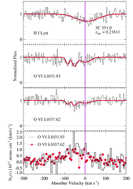
Figure 42.— Continuum-normalized absorption profiles of the H I Ly$\alpha$ and O VI $\lambda\lambda$1031.93,1037.62 lines at $z_{\rm abs}$ = 0.21811 in the spectrum of 3C 351.0 (upper three panels), and comparison of the O VI $N_{\rm a}(v)$ profiles (lowest panel). Voigt-profile fits (see Table 3) are overplotted with smooth lines. In this figure, the $N_{\rm a}(v)$ profiles are binned to 7 km s^-1 pixels, but the absorption profiles are shown at full resolution ($\approx 3.5$ km s^-1 pixels).

Appendix A Appendix: Comments on Line Identification, Blending, Hot Pixel Contamination, and Saturation in Invididual Systems

(1.) 3C 249.1, $z_{abs}$ = 0.24676. In this system, H I Ly$\beta$ is mildly blended with an unrelated line. However, most of the Ly$\beta$ profile is free from the blend, and the unblended portion of Ly$\beta$ provides useful contraints and was included in the fit. Hot pixels are present in the STIS spectrum on both the blue and red sides of the O VI $\lambda$1037.62 line (see Figure 6). The O VI identification is secure because the $\lambda$1031.93 and $\lambda$1037.62 profiles agree well in the regions that are not affected by hot pixels. However, the regions affected by hot pixels were excluded from the fit.

(2.) 3C 249.1, $z_{abs}$ = 0.30811. Both lines of the O VI doublet are detected at high significance at this redshift (see Figure 8). However, the O VI profiles are strongly saturated in the component at $v$ = 0 km s^-1. In addition, hot pixels are present in the core of the O VI $\lambda 1031.93$ line. Consequently, the line parameters are highly uncertain for the $v$ = 0 km s^-1 component.

(3.) 3C 249.1, $z_{abs}$ = 0.31364. The O VI $\lambda$1037.62 line at this redshift is only detected at the 1.9$\sigma$ level. However, the strength of the 2$\sigma$ feature is in good agreement with the expected strength implied by the well-detected O VI $\lambda$1031.93 line. In addition, the O VI $\lambda$1031.93 line is well-aligned with the H I Ly$\alpha$, Ly$\beta$, and Ly$\gamma$ lines detected at this redshift. The metal profiles marginally suggest the presence of a second component, but better S/N is required to verify and measure the second component.

(4.) 3C 273.0, $z_{abs}$ = 0.00334. The blue side of the Ly$\beta$ profile is blended with a Galactic H₂ absorption line (see Sembach et al. 2001). Consequently, only the red side of the Ly$\beta$ line (which is free from blending) was used to constrain the fit. The O VI $\lambda$1037.62 line is severely blended with Galactic H₂ absorption, so only the O VI $\lambda$1031.93 line can be measured. The O VI $\lambda$1031.93 line is affiliated with a well-detected H I absorber at the same redshift (Sembach et al. 2001). This absorber clearly shows evidence of multiple components in the H I Ly$\alpha$ profile (see Figure 37). The O VI profile, on the other hand, only shows one clear component. However, the O VI line is broad and shallow, and the breadth of the O VI feature is consistent with the velocity range spanned by the H I absorption. The degree of velocity-centroid alignment of the O VI with H I is ambiguous: the O VI is aligned, to within the 2$\sigma$ uncertainty, with both H I components derived from profile fitting in Table 3. Following the conventions outlined in §2.3.2, we assign the O VI to the broader H I component. In addition, as discussed in §4.2, the breadth of the H I component at $v=-8$ km s^-1 depends critically on the number of components assumed for the fit.

(5.) 3C 273.0, $z_{abs}$ = 0.12003. At this redshift, the O VI doublet is covered by both the STIS and the FUSE spectrum of 3C 273.0. Both lines of the O VI doublet are clearly detected in the FUSE spectrum of 3C 273.0 (see Figure 3 in Tripp et al. 2006b). In the STIS spectrum, the O VI lines are located in a region of rapidly decreasing signal-to-noise. The STIS spectrum shows the O VI 1037.62 line at 4.0$\sigma$ significance, but the significance of the 1031.93 line is $<2\sigma$. Consequently, we base our fit on the FUSE data, but we note that fitting the STIS data yeilds consistent (but noisier) results.

(6.) 3C 273.0, $z_{abs}$ = 0.15779. The O VI 1031.93 line is detected at 4.5$\sigma$ significance, but the weaker O VI $\lambda$1037.62 line is not detected. The O VI identification is favored based on the precise alignment of O VI $\lambda$1031.93 candidate with an H I Ly$\alpha$ line at the same redshift (see Figure 20).

(7.) 3C 351.0, $z_{abs}$ = 0.21811. Figure 42 shows the H I Ly$\alpha$ and O VI lines that we detect in this system; the upper panels show the absorption profiles and the lowest panel compares the O VI $N_{\rm a}(v)$ profiles. The O VI $\lambda\lambda 1031.93,1037.62$ lines are detected at the 5.5$\sigma$ and 3.7$\sigma$ levels, respectively, and the $N_{\rm a}(v)$ profiles are in good agreement. The O VI profiles are broad and shallow and hence are sensitive to continuum placement. Thom & Chen (2008) do not agree with this system identification; the most likely source of this discrepancy is continuum placement, but differences in data reduction procedures could play a role. Higher S/N observations with COS would be valuable for confirmation of broad and shallow lines such as these. Similar component structure is evident in the O VI $\lambda$1031.93 and O VI $\lambda$1037.62 profiles, and the similarity of the component structure favors a multicomponent fit. However, the O VI profiles are moderately noisy. We flag these measurements with a colon because while three components are suggested by the O VI data, better S/N is needed to robustly establish that three components are present. If we fit the O VI lines with a single component instead of the three-component fit listed in Table 3, we obtain $b$(O VI) = 82$\pm$13 km s^-1 and log $N$(O VI) = 14.06$\pm$0.05 for the single line.

(8.) 3C 351.0, $z_{abs}$ = 0.22111. An archival FUSE spectrum of 3C 351.0 shows that this is an optically-thick Lyman limit absorber with $N$(H I) $>10^{17}$ cm^-2. The Ly$\alpha$ profile is strongly saturated but shows complex structure at the edges of the profile. This structure could be partly due to damping wings, but this profile structure cannot be unambigously attributed to damping wings. Consequently, the H I column density is highly uncertain. The O VI $\lambda$1031.93 line is severely blended with the Galactic Si II $\lambda$1260.42 line, and consequently $\lambda$1031.93 cannot be measured. However, many metal lines are detected at the redshift of this strong Lyman limit system including transitions of C II, N II, Si II, Si III, and Si IV. The O VI $\lambda$1037.62 line is identified based on its alignment with the other metals at this redshift. All available H I lines are strongly saturated at the velocities of the metal lines, so the degree of alignment of the O VI and H I lines cannot be evaluated. However, analysis of the low- and high-ionization metals lines indicates the presence of multiple phases, so this system is classified as a complex absorber.

(9.) H1821+643, $z_{abs}$ = 0.02438. H I Ly$\beta$ is mildly blended with a Galactic H₂ absorption line (see Sembach et al. 2008), but the Ly$\beta$ line is mostly free from the blend. The blended portion of Ly$\beta$ was excluded from the fit. O VI $\lambda$1037.62 is lost in a blend with Milky Way Fe II and H₂ absorption. The O VI identification is based on the precise alignment of O VI $\lambda$1031.93 with Ly$\alpha$ and Ly$\beta$ lines at the same redshift.

(10.) H1821+643, $z_{abs}$ = 0.12143. Thom & Chen (2008) challenge this O VI identification, noting that “there is strong absorption at the O VI 1037 position, but no O VI 1031, which should be easily detected, given the strength of the weaker supposed O VI 1037 line.” However, as discussed in detail by Tripp et al. (2001), the O VI $\lambda$1037.62 line is significantly blended with strong H I Ly$\delta$ absorption from the absorber at $z_{\rm abs}$ = 0.22496 (see Figure 2 in Tripp et al. 2001), and it appears that Thom & Chen (2008) have not taken this serious blend into account. Moreover, Thom & Chen base their conclusions on the STIS data only, which have S/N $\lesssim$ 3 per pixel in this wavelength range, whereas the FUSE observations we used have S/N $\gtrsim$ 13 per pixel here. When the FUSE data are employed and the Ly$\delta$ blend is accounted for, we find compelling evidence supporting this system. Because of the strong blend, our O VI measurements are based on the 1031.93 line alone. The O VI $\lambda$1031.93 line is detected at the 6.9$\sigma$ level in our data. While the blend hampers confirmation based on the 1037.63 line, we note that there are no other clear identifications for the 6.9$\sigma$ line at the 1031.93 wavelength. This is not an H I Ly$\alpha$ line because the redshift places the line blueward of the Ly$\alpha$ region, nor is it a higher Lyman series H I line because corresponding strong H I lines would be obvious in the STIS spectrum but are not evident.

(11.) H1821+643, $z_{abs}$ = 0.21331. The O VI $\lambda$1037.62 line is blended with weak, high-velocity S II $\lambda$1259.52 absorption from Milky Way gas (see Savage et al. 1995 and Tripp et al. 2003 for information about the Galactic high-velocity gas toward H1821+643). Comparison of the Galactic S II $\lambda$1259.52 and S II $\lambda$1253.81 lines shows that there is excess optical depth in the 1259.52 Å line, and the excess is consistent with the expected contribution from the O VI $\lambda$1037.62 line at $z_{\rm abs}$ = 0.21331 (based on the strength of the unblended O VI $\lambda$1031.93 line), which supports the identification of O VI at this redshift. In addition, the O VI $\lambda$1031.93 line is aligned with H I Ly$\alpha,\beta,\ {\rm and}\ \gamma$ lines at the same $z_{\rm abs}$.

(12.) HE0226-4110, $z_{abs}$ = 0.01747. The O VI $\lambda$1037.62 line is blended with O IV $\lambda$787.71 at $z_{\rm abs}$ = 0.34035 (see Lehner et al. 2006 and Figure 33). The O VI identification is favored based on the precise alignment of O VI $\lambda$1031.93 candidate with an H I Ly$\alpha$ line at the same redshift. We note that the comparison of the $N_{\rm a}$ profiles in Figure 20 does not show the absorption in the wings of the Ly$\alpha$ line very clearly; Figure 33 more clearly shows how the H I line is slightly broader than the O VI lines.

(13.) HE0226-4110, $z_{abs}$ = 0.20701. Detailed analysis of this system has been presented by Savage et al. (2005). The H I Ly$\gamma$ line is recorded in both the STIS spectrum and the FUSE spectrum of HE0226-4110. The apparent component structure in the STIS recording of the Ly$\gamma$ line is incompatible with the FUSE recording of Ly$\gamma$ and with the other (higher) Lyman series lines (see Savage et al. 2005), and the STIS Ly$\gamma$ line was excluded from the fit.

(14.) HE0226-4110, $z_{abs}$ = 0.35525. A weaker line offset by +40 km s^-1 is present next to the main component that is clearly detected in the O VI $\lambda$1031.93 and O VI $\lambda$1037.62 profiles at this redshift. The +40 km s^-1 feature does not appear to be O VI because it is not confirmed by the $\lambda$1037.62 line. However, the +40 km s^-1 feature would be relatively weak in the $\lambda$1037.62 transition, and it could be hidden by noise. Following Lehner et al. (2006), we do not include the 40 km s^-1 component in the O VI measurements; higher S/N data are needed to establish the identity of this feature.

(15.) HE0226-4110, $z_{abs}$ = 0.42670. At this redshift, the Ly$\alpha$ is redshifted beyond the long-wavelength cutoff of our STIS spectrum, and Ly$\beta$ line is not detected. The O VI identification is based on the good agreement of the O VI $\lambda$1031.93 and $\lambda$1037.62 profiles (see Lehner et al. 2006). The O VI $\lambda$1031.93 line is partially affected by hot pixels that were excluded from the fit. We note that identification of this system depends critically on the STIS warm/hot pixel correction algorithm. If we turn off the hot-pixel repair algorithm, we find that the O VI $\lambda$1037.62 line is largely filled in by warm pixels. It is important to obtain future observations of this system with COS in order to test the reliability of the identification and to expand the utility of this system with additional information (e.g., better H I absorption constraints).

(16.) HE0226-4110, $z_{abs}$ = 0.49246. This complex, multispecies system has been analyzed in detail by Ganguly et al. (2006). The O VI component at $v=0$ km s^-1 is uncertain due to substantial saturation. The O VI $\lambda$1037.62 line is partially blended with Galactic C IV (see Fox et al. 2005), but the distinctive component structure seen in the O VI $\lambda$1031.93 profile can be clearly recognized in the in the $\lambda$1037.62 profile as well (see Ganguly et al. 2006), so the identification is secure, and the weaker O VI components are well-constrained by the O VI $\lambda$1031.93 line.

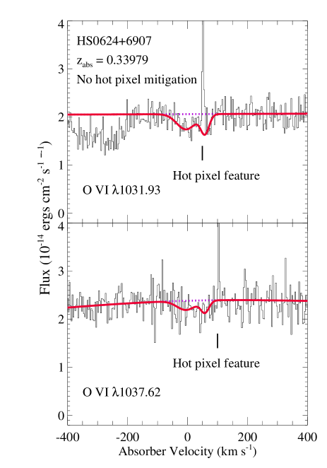
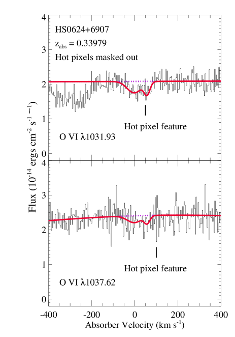
Figure 43.— Demonstration of hot pixel alleviation by masking (rejection) of affected regions in individual exposures. The panels show the regions of the O VI $\lambda$1031.93 line (top panels) and the O VI $\lambda$1037.62 line (bottom panels) at $z_{\rm abs}$ = 0.33979 in the spectrum of HS0624+6907. The left panels show the line profiles without any hot pixel alleviation; hot pixels are clearly evident near both profiles. The HS0624+6907 observations were recorded in Jan. 2002 and Feb. 2002 (see Table 1), and the spectrum position on the detector was shifted between the two dates. Consequently, the hot pixels are only present in the February data and can be masked and rejected from the final coadded spectrum as shown at right.

(17.) HS0624+6907, $z_{abs}$ = 0.33979. H I Ly$\beta$ is mildly blended with an unrelated line. However, most of the Ly$\beta$ profile is free from the blend, and the unblended portion of Ly$\beta$ was included in the fit. As shown in the left panel of Figure 43, hox pixel features are present within the O VI $\lambda$1031.93 line and at the red edge of the O VI $\lambda$1037.62 profile. Fortunately, in this case the QSO was observed on two different dates (in January 2002 and February 2002, see Table 1), and the position of the spectrum on the detector was shifted between these two dates. Inspection of the data reveals that the hot pixel features are only present in the February 2002 data. As shown in the right panel of Figure 43, by masking and rejecting the affected hot pixels in the February data, we can suppress this problem with a minimal loss of the signal-to-noise.

(18.) HS0624+6907, $z_{abs}$ = 0.37053. In this proximate absorber, H I Ly$\alpha$ is not detected despite good signal-to-noise (see Figure 8). As shown in Figure 8, the O VI identification is quite secure; both lines of the O VI doublet show multiple components and are in excellent agreement.

(19.) PG0953+415, $z_{abs}$ = 0.06807. We have carried out extensive investigations of this absorber in previous papers (Savage et al. 2002; Tripp et al. 2006). Comparison of the O VI $\lambda$1031.93 and $\lambda$1037.62 lines indicates moderate saturation, and application of the method of Jenkins (1996) indicates that $N$(O VI) could be 0.25 dex higher.

(20.) PG0953+415, $z_{abs}$ = 0.14231. The Ly$\beta$ profile is partially blended with an H I Ly$\delta$ line from $z_{\rm abs}$ = 0.23351. The blended part of the Ly$\beta$ line was not used in the fit. However, the Ly$\alpha$ line has a complex profile with many components (see Tripp & Savage 2000), and the unblended portion of the Ly$\beta$ line provides useful constraints for the fit.

(21.) PG0953+415, $z_{abs}$ = 0.22974. In this proximate absorber of PG0953+415, H I Ly$\alpha$ is not detected despite good signal-to-noise. The O VI identification is based on the good agreement of the O VI lines over a large portion of both profiles: the $\lambda$1031.93 and $\lambda$1037.62 profiles agree well over $\approx 20$ pixels between $v=-30$ km s^-1 and $v=40$ km s^-1. However, the O VI profiles are discrepant at $v<-30$ km s^-1. While this discrepancy has the appearance of a hot pixel feature, comparison of the data from 1998 December 4 and 1998 December 11 shows the same profile structure. The location of the spectrum on the detector was shifted between 1998 December 4 and 1998 December 11, so this discrepancy cannot be due to hot pixels. We conclude that the O VI $\lambda$1031.93 line is blended with an unrelated Ly$\alpha$ line on the blue side of the profile. This part of the $\lambda$1031.93 profile was excluded from the Voigt profile fit.

(22.) PG0953+415, $z_{abs}$ = 0.23351. A Ly$\delta$ line with approximately correct strength is detected at this redshift but was not used in the fit due to blending with Ly$\beta$ from the complex, multicomponent absorber at $z_{\rm abs}$ = 0.14231.

(23.) PG1116+215, $z_{abs}$ = 0.05927. Both lines of the O VI doublet are detected and in excellent agreement at $v=0$ km s^-1 (see Figure 33). The O VI $\lambda$1031.93 line is also detected at $v=-84$ km s^-1, but the O VI $\lambda$1037.62 line is not significantly detected at that velocity. A small portion of the detected O VI $\lambda$1031.93 component at $v=-84$ km s^-1 is blended with Galactic H₂ (see Sembach et al. 2004). The $v=-84$ km s^-1 component is also identified as O VI based on the good agreement of the O VI and H I Ly$\alpha$ line shapes at $v=-84$ km s^-1 (not including the portion blended with H₂, which was also excluded from the fit), as shown in Figure 20.

(24.) PG1116+215, $z_{abs}$ = 0.13849. The O VI doublet at this redshift is detected with both FUSE and STIS (see Sembach et al. 2004). The fit reported here is based on the STIS data. This system, which has a high H I column and is detected in many Lyman series lines, has been analyzed in detail by Sembach et al. (2004). The O VI lines are aligned with the H I lines, but analysis of the many low-ionization metal absorption lines detected in this system clearly establishes that this is a complex multiphase absorber (see Sembach et al. 2004).

(25.) PG1116+215, $z_{abs}$ = 0.16553. The H I components at $v=-12,143,170,$ and 342 km s^-1 are well-constrained by the detected absorption lines. Additional absorption is clearly and significantly detected in other velocity ranges in the Ly$\alpha$ profile, e.g., at $v\approx$ 70 km s^-1, and components were added to the fit to account for this additional absorption. However, these components are not well-constrained due to blending with the adjacent features.

(26.) PG1116+215, $z_{abs}$ = 0.17340. The O VI $\lambda$1031.93 line is detected at 5.8$\sigma$ significance and is well-aligned with an H I line at the same redshift. In addition, the O VI $\lambda$1037.62 line is detected with the expected wavelength and relative strength at 2.9$\sigma$.

(27.) PG1216+069, $z_{abs}$ = 0.12360. The Ly$\alpha$ profile has good signal-to-noise and shows clear inflections and asymmetries that reveal the complicated component structure including at least eight components; four of the components are clearly evident in the Ly$\beta$ profile as well (see Figure 4). However, all of the components are either strong and significantly saturated (in both Ly$\alpha$ and Ly$\beta$) or are highly blended with adjacent strong components. Moreover, some of the saturated components show that there are errors in the flux zero level of the Ly$\alpha$ line, and the Ly$\beta$ line is relatively noisy. Ly$\gamma$ lines are also evident (see Tripp et al. 2005), but the Ly$\gamma$ data are too noisy to usefully constrain the fits. The H I component parameters are highly uncertain due to these combined problems. Both lines of the O VI doublet are strong and are clearly detected with component structure similar to the Ly$\beta$ components. The apparent column density profiles of the O VI doublet are in good agreement (see Figure 4), which suggests that the O VI lines are not badly saturated. However, the O VI profiles are also relatively noisy.

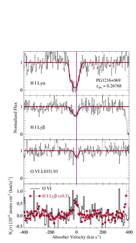
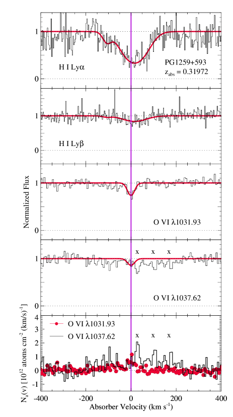
Figure 44.— Left panels: Continuum-normalized absorption profiles of the H I Ly$\alpha$, Ly$\beta$, and O VI $\lambda$1031.93 lines at $z_{\rm abs}$ = 0.26768 in the spectrum of PG1216+069 (upper three panels), and comparison of the O VI $\lambda$1031.93 and Ly$\beta$ $N_{\rm a}(v)$ profiles (lowest panel). Voigt-profile fits (see Table 3) are overplotted with smooth lines. As in other figures, unrelated lines are marked with an ‘x’. Right panels: Absorption profiles of the H I and O VI lines detected at $z_{\rm abs}$ = 0.31972 in the spectrum of PG1259+593. In this stack, the lowest panel compares the $N_{\rm a}(v)$ profiles of the O VI $\lambda$1031.93 and $\lambda$1037.62 lines. In this figure, the $N_{\rm a}(v)$ profiles are binned to 7 km s^-1 pixels.

(28.) PG1216+069, $z_{abs}$ = 0.26768. The O VI $\lambda$1037.62 line cannot be measured because it is lost in a blend with a strongly saturated H I Ly$\beta$ absorption line from $z_{\rm abs}$ = 0.28189. As shown in Figure 44, the O VI identification at $z_{\rm abs}$ = 0.26768 is based on the alignment of O VI $\lambda$1031.93 with Ly$\alpha$ and Ly$\beta$ at the same redshift. At this redshift, initial inspection indentified a candidate C III $\lambda$977.02 line that is somewhat blended with N V $\lambda$1238.82 absorption from the Milky Way. The C III candidate cannot be a second component of Galactic N V absorption because it is not evident in the profile of the other line of the N V doublet. However, closer inspection reveals that this line is not C III but rather is the H I Ly$\gamma$ line from the strong H I system at $z_{\rm abs}$ = 0.27353, so we can only place an upper limit on C III absorption at this redshift.

(29.) PG1259+593, $z_{abs}$ = 0.04637. Only the O VI $\lambda$1031.93 line is detected at this redshift (O VI $\lambda$1037.62 is redshifted into a relatively noisy region of the FUSE spectrum that is only recorded by the SiC channels). Nevertheless, the identification is secure because the O VI $\lambda$1031.93 profile has a distinctive two-component structure that matches the component structure seen in the C III and C IV lines detected at the same redshift. An unrelated O IV $\lambda$787.71 line is located near the Ly$\gamma$ profile; the region affected by the O IV feature was excluded from the fit.

(30.) PG1259+593, $z_{abs}$ = 0.21949. Several components due to Galactic S II $\lambda$1250.58 are located on the blue side of the Ly$\beta$ line (see Richter et al. 2004); the velocity range affected by the Milky Way S II absorption was excluded from the fit.

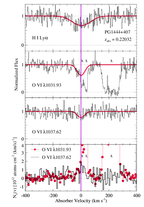
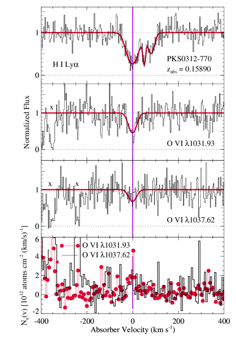
Figure 45.— Left panels: Continuum-normalized absorption profiles of the H I Ly$\alpha$ and O VI $\lambda\lambda$1031.93, 1037.62 lines at $z_{\rm abs}$ = 0.22032 in the spectrum of PG1444+407 (upper three panels), and comparison of the O VI $\lambda$1031.93 and $\lambda$1037.62 $N_{\rm a}(v)$ profiles (lowest panel). Voigt-profile fits (see Table 3) are overplotted with smooth lines. Unrelated lines are marked with an ‘x’. The O VI $\lambda$1031.93 line is blended with Milky Way S II $\lambda$1259.52 absorption, but excess absorption is present in the blend that cannot be attributed to S II. As shown, the excess absorption is consistent with the expected strength of the O VI $\lambda$1031.93 line. Right panels: The same data for the O VI absorber at $z_{\rm abs}$ = 0.15890 in the spectrum of PKS0312-770. In this figure, the $N_{\rm a}(v)$ profiles are binned to 7 km s^-1 pixels.

(31.) PG1259+593, $z_{abs}$ = 0.31972. The O VI $\lambda$1037.62 line is quite weak and mildly blended with high-velocity Ni II absorption from the Milky Way (see Richter et al. 2004). As shown in the right panels of Figure 44, the O VI $\lambda 1031.93$ line is clearly detected, and an absorption feature with the right relative strength (compared to $\lambda$1031.93) is present at the expected wavelength of O VI $\lambda$1037.62, but because it is weak and blended with Galactic Ni II, our fit is based on the O VI $\lambda$1031.93 line only.

(32.) PG1444+407, $z_{abs}$ = 0.22032. The H I Ly$\alpha$ and O VI $\lambda\lambda$1031.93, 1037.62 lines for this absorption system are shown in the left panels of Figure 45. The O VI $\lambda$1031.93 line at $z_{abs}$ = 0.22032 is blended with the Galactic S II $\lambda$1259.52 line. However, comparison of the Galactic S II 1253.81 and S II $\lambda$1259.52 profiles shows a clear and significant excess of absorption at the expected velocity of O VI $\lambda$1031.93 at $z_{\rm abs}$ = 0.22032. Moreover, the excess absorption has precisely the expected strength compared to the (unblended) O VI $\lambda$ 1037.62 line, as can be seen in the comparison of the O VI $N_{\rm a}(v)$ profiles shown in Figure 45. Only the unblended portion of O VI $\lambda$1031.93 was included in the fit.

(33.) PG1444+407, $z_{abs}$ = 0.26738. The Ly$\beta$ line is slightly blended with an unrelated weak line; the region affected by the blend was excluded from the fit. More importantly, the Ly$\alpha$ line is located at the peak of the broad Ly$\alpha$ emission line, and this introduces significant continuum placement uncertainty. We note that a broad and shallow feature is located just blueward of the Ly$\alpha$ line. This feature could be due to additional weak H I absorption, but its significance is highly dependent on the uncertain continuum placement. Consequently, we did not include the broad, shallow feature in the fit.

(34.) PHL1811, $z_{abs}$ = 0.07765. Only the stronger O VI $\lambda$1031.93 line is detected at $>3\sigma$ significance. However, many metals are detected at this redshift including C II $\lambda 1334.53$, Si II $\lambda 1260.42$, C III $\lambda 977.02$, C IV $\lambda 1548.20$, (marginal) Si IV $\lambda 1393.76$, and several H I Lyman series lines. The strongest C IV component shows a $\approx-25$ km s^-1 offset from the lower ionization metals, but the O VI $\lambda$1031.93 line is aligned with the C IV $\lambda$1548.20 transition.

(35.) PHL1811, $z_{abs}$ = 0.15786. The Ly$\alpha$ profile at $z_{\rm abs}$ = 0.15786 is blended with O I $\lambda$1302.17 absorption from the Lyman-limit system at $z_{\rm abs}$ = 0.08092 (see Jenkins et al. 2005 and Figure 39). The narrow core in this blend is predominantly due to the Lyman-limit O I line. However, close inspection of this profile (see Figure 39) reveals weak component absorption straddling the narrow core on the short- and long-wavelength sides. We cannot corroborate that the weaker components are also O I; similar component structure is not clearly evident in the other profiles of low-ionization metals in this Lyman-limit absorber, which suggests that these weaker components could be unrelated to the O I and could be Ly$\alpha$ at $z_{\rm abs}$ = 0.15786. However, better S/N data are needed to reliably determine the origin of the weak components and to accurately deblend and measure their parameters, so we flag this absorption with a colon in Table 3 to reflect the substantial uncertainty of this Ly$\alpha$ case.

(36.) PHL1811, $z_{abs}$ = 0.17650. At this redshift, O VI $\lambda 1031.93$ falls in the saturated core of the Milky Way damped Ly$\alpha$ line. The O VI $\lambda 1037.62$ line is identified based on its alignment with multiple Lyman series lines, and this is supported by the detection of C III $\lambda 977.02$ and Si III $\lambda 1206.5$ in this absorber. However, we note that the O VI is offset by $\sim-25$ km s^-1 compared to the C III and Si III lines.

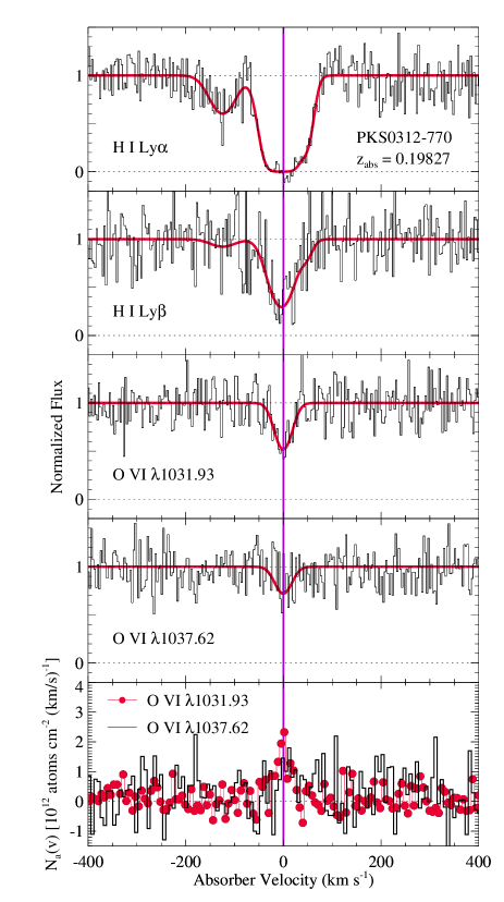
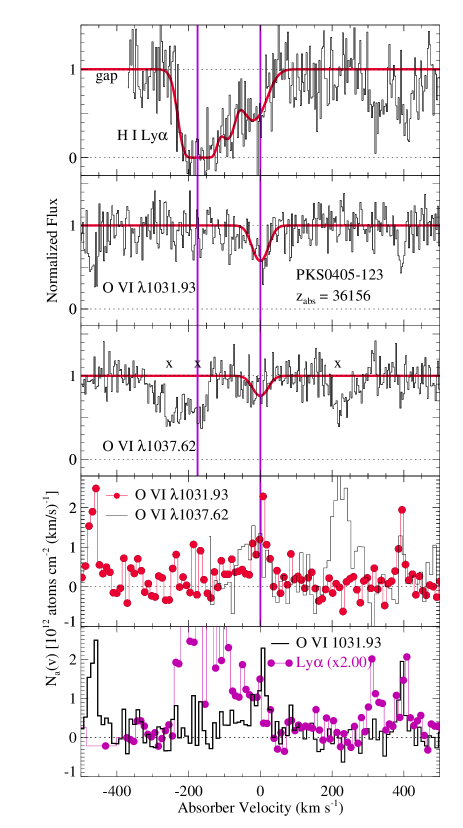
Figure 46.— Left panels: Continuum-normalized absorption profiles of the H I Ly$\alpha$, Ly$\beta$, and O VI $\lambda\lambda$1031.93, 1037.62 lines at $z_{\rm abs}$ = 0.19827 in the spectrum of PKS0312-770 (upper four panels), and comparison of the O VI $\lambda$1031.93 and $\lambda$1037.62 $N_{\rm a}(v)$ profiles (lowest panel). Voigt-profile fits (see Table 3) are overlaid with smooth lines. Right panels: Same data for the absorber at $z_{\rm abs}$ = 0.36156 in the spectrum of PKS0405-123. In this stack, the lowest two panels show the comparison of the $N_{\rm a}(v)$ profiles of the two lines of the O VI doublet (second panel from bottom) and a comparison of the O VI $\lambda 1031.93$ and H I Ly$\alpha$ $N_{\rm a}(v)$ profiles (lowest panel). Unrelated lines are marked with an ‘x’. In this figure, the $N_{\rm a}(v)$ profiles are binned to 7 km s^-1 pixels.

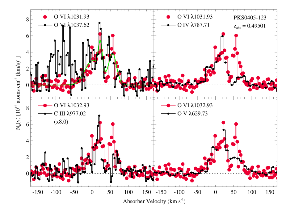
Figure 47.— Comparison of apparent column density profiles of several metals in the O VI absorption system at $z_{\rm abs}$ = 0.49501 in the spectrum of PKS0405-123. Upper left: O VI $\lambda$1031.93 (red large circles) vs. O VI $\lambda$1037.62 (small black circles). The thick green line shows the O VI profile implied by the Voigt-profile fit listed in Table 3. Upper right: O VI $\lambda$1031.93 (red large circles) vs. O IV $\lambda$787.71. Lower left: O VI $\lambda$1031.93 (red large circles) vs. C III $\lambda$977.02. Lower right: O VI $\lambda$1031.93 (red large circles) vs. O V $\lambda$629.73. Several pixels are not plotted in the core of the O V profile because it is saturated in that region. The O IV and O V profiles are from the FUSE observations reported by Prochaska et al. (2004), and the C III and O VI data are measured from the STIS E140M spectrum. Most of these profiles show two weaker components flanking the deepest central component, but as discussed in the text, an offset is apparent between the peak of the O VI $\lambda$1031.93 and $\lambda$1037.62 lines in the reddest component.

(37.) PKS0312-770, $z_{abs}$ = 0.15890. O VI $\lambda$1031.93 is detected at 5.6$\sigma$ significance, and the corresponding O VI $\lambda$1037.62 line is also detected, but only at 2.4$\sigma$ significance. As shown in Figure 45, the $N_{\rm a}(v)$ profiles of the two lines of the O VI doublet are in good agreement, and the marginal detection of the $\lambda$1037.62 line supports the O VI identification. The O VI identification is also supported by the precise alignment of the O VI $\lambda$1031.93 line with H I Ly$\alpha$ at the same redshift.

(38.) PKS0312-770, $z_{abs}$ = 0.19827. O VI $\lambda$1031.93 is detected at 4.7$\sigma$ significance, but the O VI $\lambda$1037.62 line is not significantly detected in the data at full resolution. However, as shown in the left panels of Figure 46, if we mildly bin the data to 7 km s^-1 pixels to improve the S/N, we find a feature in the spectrum at the expected wavelength of the $\lambda$1037.62 line that is fully consistent with the detected O VI $\lambda$1031.93 line (compare the $N_{\rm a}(v)$ profiles shown in the lowest left-hand panel of Figure 46). The O VI identification is bolstered by the close alignment of O VI $\lambda$1031.93 with Ly$\alpha$ and Ly$\beta$ at the same redshift (see the left panels in Figure 46).

(39.) PKS0312-770, $z_{abs}$ = 0.20266. All accessible H I lines in the STIS bandpass (Ly$\alpha$, Ly$\beta$, Ly$\gamma$) are strong and highly saturated. Moreover, the Ly$\beta$ and Ly$\gamma$ profiles show complex component structure with at least five distinct components. Since most of the H I components are black in the line cores, the H I profile parameters are poorly constrained, and we have not attempted to fit the H I lines. Brief inspection of an archival FUSE spectrum reveals that this is an optically thick Lyman limit absorber. While the H I component properties are poorly constrained, comparison of the low- and high-ionization metal lines reveals that this is a complex multiphase system (see §2.4.1 and Figure 3). In addition, the individual components are spread over a large velocity range with low- and high-ionization components detected at velocities ranging from $-204$ to +135 km s^-1.

(40.) PKS0405-123, $z_{abs}$ = 0.16692. Many Lyman series lines are available for constraining the H I column density at this redshift, and the absence of strong Lyman limit absorption places a firm upper limit on the total H I column density (Prochaska et al. 2004). Nevertheless, the parameters of the individual H I components are highly uncertain in this system. The Lyman series lines clearly require a multicomponent fit, but the close spacing and blending of the components causes the component parameter uncertainties to be substantial. Thus, the degree of alignment of the H I and O VI components is highly uncertain. Nevertheless, comparison on the low- and high-ionization metal lines shows that this is a complex multiphase case (see Chen & Prochaska 2000).

(41.) PKS0405-123, $z_{abs}$ = 0.36156. The H I Ly$\alpha$ and O VI $\lambda\lambda$1031.93, 1037.62 absorption profiles and apparent column densities are compared in the right-hand stack of Figure 46. The O VI $N_{\rm a}(v)$ profiles are seen to be in reasonable agreement. We note that the O VI $\lambda$1037.62 profile shows a small excess of absorption on the blue side compared to the $\lambda$1031.93 line; this could be due to blending with an unrelated line (several unrelated lines are readily apparent in the vicinity of $\lambda$1037.62), but this could also simply be a noise feature. An inflection is also evident in the Ly$\alpha$ profile at the velocity of the O VI lines. It is interesting to note that this system has a relatively high $N$(H I) and is detected in several Lyman series lines, but no O VI absorption is evident at the velocity of the main component where the strong H I lines are found (see Figure 46). Instead, the O VI is in the wing of the profile near the weak H I inflection component. Several other absorbers show similar offsets between the strong main H I absorption component and the O VI lines (see Figure 20).

(42.) PKS0405-123, $z_{abs}$ = 0.36335. The O VI $\lambda$1031.93 line is detected at the 4.5$\sigma$ level, but O VI $\lambda$1037.62 is measured at only 1.7$\sigma$ significance. However, the apparent column density profiles of the two O VI lines agree precisely; the wavelength separation and relative strength of the lines makes the O VI identification compelling. The corresponding H I absorption is relatively weak, and moreover, the H I Ly$\alpha$ line is strongly blended with Galactic C I and C I* absorption lines from the C I $\lambda$1656 multiplet. We can see that H I Ly$\alpha$ absorption is present at this redshift because the Galactic C I* $\lambda$1657.38 line is clearly too strong compared to other C I* lines in the PKS0405-123 spectrum. However, the H I Ly$\alpha$ line is difficult to measure reliably due to this strong blending with Galactic C I* $\lambda$1657.38.

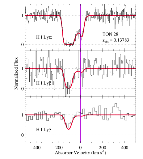
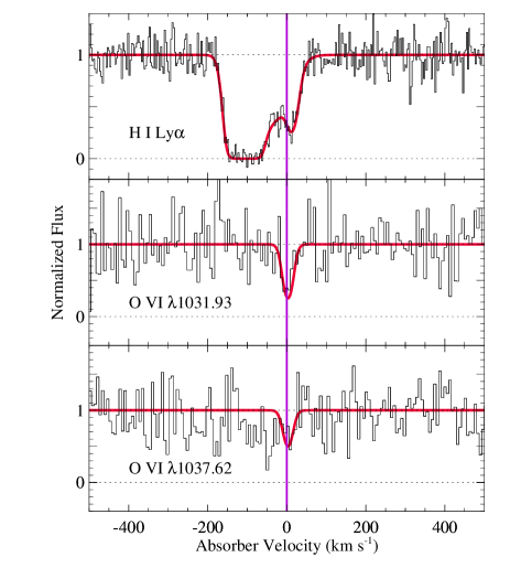
Figure 48.— Left panels: Continuum-normalized absorption profiles of the H I Ly$\alpha,\beta,\gamma$ and O VI $\lambda\lambda$1031.93,1037.62 lines in the absorption system at $z_{\rm abs}$ = 0.13783 toward TON28.

(43.) PKS0405-123, $z_{abs}$ = 0.49501. In this case, the H I Ly$\alpha$ line is redshifted beyond the long wavelength cutoff of the STIS spectrum, but Ly$\beta$ and Ly$\gamma$ are detected at the 4.1$\sigma$ and 2.0$\sigma$ levels, respectively. This absorber is detected in a variety of metals (Prochaska et al. 2004), and many of the metal profiles, including the O VI lines, show evidence of multiple components. However, it should be noted that there is a discrepancy evident in one of the components of the O VI $\lambda\lambda$1031.93,1037.62 lines. To show this, we compare the apparent column density profiles of the O VI $\lambda\lambda$1031.93,1037.62 lines in Figure 47. We also compare the O VI $\lambda$1031.93 $N_{\rm a}(v)$ profile to those of C III $\lambda$977.02, O IV $\lambda$787.71, and O V $\lambda$629.73 in Figure 47. The O VI The O VI $\lambda$1031.93 and $\lambda$1037.62 profiles agree well in the stronger component at $v\approx$ 0 km s^-1. Looking closely at the strongest component, we can see that the profile is asymmetric with a sharp edge on the red side and a more gradually decreasing apparent column density on the blue side. This asymmetry suggests that the main feature is a blend of two components, and this is corroborated by the C III and O IV profiles, which also show an extra component on the blue side. A third component is evident at $v\approx$ 70 km s^-1 in the C III and O IV transitions. This component appears to be present in the O V and O VI profiles as well, but at a somewhat lower velocity ($v=57$ km s^-1). However, there is a $2-3$ pixel offset between the peak of the O VI $\lambda$1031.93 and O VI $\lambda$1037.62 profiles in the $v=57$ km s^-1 component (see Figure 47), in contrast to the $v\approx$ 0 km s^-1 component in which the O VI profiles agree well. Initially, this offset appeared to be due to a hot pixel feature falling in the middle of the O VI $\lambda$1031.93 line, but this cannot be the cause because the PKS0405-123 observations were obtained on two separate occasions (see Table 1), and the spectrum detector position was shifted between the two visits. The same component structure is evident in the O VI profiles extracted separately from the two visits, so this problem is not due to a hot-pixel feature. Apart from this small offset, the $N_{\rm a}(v)$ profiles of the O VI lines at $v=57$ km s^-1 appear to be quite consistent: the relative strength and shape of the two lines are in agreement. This suggests that the offset could be caused by an instrumental calibration problem. For example, the STIS geometric distortion can cause offsets of this magnitude if not properly corrected (Walsh et al. 2001; Maíz-Apellániz & Úbeda 2004), and some problems with the distortion correction have been noted (Maíz-Apellániz & Úbeda 2004). Evidence of wavelength calibration problems have also been noted when comparing lines that should have identical component structure (e.g., Jenkins & Tripp 2001; Tripp et al. 2005). While we have found these problems to be relatively rare, the stability of the STIS gemometric distortion correction has not been studied systematically, and it remains possible that the discrepancy in the $v=57$ km s^-1 component is caused by a calibration problem such as this. Nevertheless, we flag the O VI lines in the $v=57$ km s^-1 component with a colon in Table 3 because of this disagreement, and we treat this component as an insecure identification. With the new Cosmic Origins Spectrograph, it will be possible to reobserve PKS0405-123 to determine if the offset is due to a STIS instrumental problem. The O VI $\lambda$1037.62 line at this redshift falls close to Galactic C IV $\lambda$1550.78 (which is the source of the extra absorption evident at $v<-40$ km s^-1 in Figure 47), but from the corresponding Galactic C IV $\lambda$1548.20 line, we can see that the Milky Way C IV has little impact on the redshifted O VI $\lambda$1037.62 profile. We give this system an uncertain classification due to the insecure identification of the O VI component at $v=57$ km s^-1 and the fact that the Ly$\alpha$ profile, which is needed to detect low-$N$(H I) components, has not been observed at high resolution.

(44.) PKS1302-102, $z_{abs}$ = 0.19159. The profile fitting code obtains its best fit to the H I lines with a narrow and deep component superimposed on a broad and shallow component at the same velocity. The absorption that requires the broad component could be nearly as well-fit with multiple narrower components, and higher S/N is required to break this degeneracy. Only O VI $\lambda$1031.93 is detected, but the O VI line is precisely aligned with the H I lines, and C III $\lambda$977.02 and Si III $\lambda$1206.50 are also detected with good significance at this redshift.

(45.) PKS1302-102, $z_{abs}$ = 0.22563. Some parts of the Ly$\beta$ profile are affected by blends; those regions of Ly$\beta$ were excluded from the fit. The O VI $\lambda$1037.62 line is also located next to an unrelated strong line. However, the O VI 1031.93 and 1037.62 $N_{\rm a}(v)$ profiles show excellent agreement over most of the velocity range where $\lambda$1031.93 is clearly detected, and the velocity range of the O VI $\lambda$1037.62 line that is affected by the adjacent interloper was excluded from the fit.

(46.) TON28, $z_{abs}$ = 0.13783. The O VI $\lambda$1037.62 line is only detected at the 2.2$\sigma$ level, but as shown in Figure 48, its wavelength and relative strength agree with the corresponding O VI $\lambda$1031.93 line. In addition, we can see from this figure that the O VI lines are aligned with a clearly detected component in the corresponding H I Ly$\alpha$ line.

(47.) TON28, $z_{abs}$ = 0.27340. The H I Ly$\alpha$ line is strongly blended with Milky Way C IV $\lambda$1548.20. However, the H I at this redshift is securely identified and measured based on the well-detected Ly$\beta$ and Ly$\gamma$ lines, and comparison of the Galactic C IV $\lambda$1548.20 and $\lambda$1550.78 apparent column density profiles verifies that substantial extra optical depth (due to the blended Ly$\alpha$ line) is present in the Galactic C IV $\lambda$1548.20 profile.

Table 1Sight Line Properties and Log of STIS E140M Echelle Observations

		Galactic Coords. and Column Densities				STIS Observations
QSO	$z_{\rm QSO}$	$l$	$b$	log $N$(H I)	log $N$(H2)	Dates	Integration	STIS	S/N
Sight Line		(deg)	(deg)			(yr.mn.dy)	Time (ksec)	Aperture	Ratio
(1)	(2)	(3)	(4)	(5)	(6)	(7)	(8)	(9)	(10)
3C 249.1	0.3115	130.4	38.5	20.45	19.09	2002.04.16	8.888	0.06$\times$0.2	12
						2002.10.03	12.168
						2002.10.04	14.496
						2002.10.05	12.168
						2002.10.08	12.168
						2002.10.09	8.888
3C 273.0	0.1583	290.0	64.4	20.22	15.92	2000.05.02	4.987	0.2$\times$0.2	33
						2000.06.21	4.987
						2000.06.22	8.697
3C 351.0	0.3719	90.1	36.4	20.2	$\cdots$	1999.06.27	19.770	0.06$\times$0.2	12
						1999.06.29	14.428
						2000.02.10	19.770
						2000.07.25	24.230
H1821+643	0.2970	94.0	27.4	20.58	15.99	1999.06.25	25.466	0.06$\times$0.2	19
						2000.03.31	25.466
HE0226–4110	0.4950	253.9	$-65.8$	20.27	14.56	2002.12.25	2.106	0.06$\times$0.2	11
						2002.12.26	16.300
						2002.12.27	6.044
						2002.12.29	8.150
						2002.12.31	11.172
HS0624+6907	0.3700	145.7	23.3	20.90	19.73	2002.01.02	14.490	0.06$\times$0.2	13
						2002.02.23	32.970
						2002.02.24	14.490
PG0953+415	0.2341	179.8	51.7	20.09	15.25	1998.12.04	10.743	0.2$\times$0.2	12
						1998.12.11	13.735
PG1116+215	0.1765	223.4	68.2	20.07	15.30	2000.05.15	7.299	0.06$\times$0.2	16
						2000.05.20	12.619
						2000.06.22	1.979
						2000.06.23	7.980
						2000.06.30	9.959
PG1216+069	0.3313	281.1	68.1	20.21	$\cdots$	2003.05.23	12.613	0.06$\times$0.2	11
						2003.05.24	10.655
						2003.06.05	7.756
						2003.06.14	7.756
						2003.06.17	15.512
						2003.06.21	7.756
						2003.06.22	7.756
PG1259+593	0.4778	120.6	58.0	20.22	14.92	2001.01.17	28.880	0.06$\times$0.2	14
						2001.01.18	28.880
						2001.01.19	23.560
						2001.12.19	14.440
PG1444+407	0.2673	69.9	62.7	20.03	$\cdots$	2002.09.09	8.104	0.06$\times$0.2	12
						2002.09.19	8.104
						2002.09.24	5.082
						2002.09.25	16.208
						2002.09.26	11.126
PHL1811	0.1900	47.5	$-44.8$	20.59	19.36	2002.10.07	10.654	0.06$\times$0.2	16
						2002.10.09	7.755
						2003.07.08	4.856
						2003.07.09	10.654
PKS0312–770	0.2230	293.4	$-37.6$	20.90	$\cdots$	2001.03.07	12.629	0.2$\times$0.2	10
						2001.05.12	12.629
						2001.10.16	12.650
PKS0405–123	0.5726	204.9	$-41.8$	20.54	16.01	1999.01.24	13.604	0.06$\times$0.2	14
						1999.03.07	13.604
PKS1302–102	0.2784	308.6	52.2	20.50	16.30	2001.08.20	11.079	0.2$\times$0.2	11
						2001.08.21	11.040
TON28	0.3297	200.1	53.2	20.25	$\cdots$	2003.04.17	7.743	0.06$\times$0.2	10
						2003.04.18	7.743
						2003.04.19	15.486
						2003.05.27	9.686
						2003.05.29	7.743

Note. — (1) Target QSO, (2) - (4) QSO redshift and Galactic coordinates from the NASA Extragalactic Database (NED), (5) total Galactic H I column density determined from 21 cm emission; all measurements are from Wakker et al. (2003) except 3C 351.0 (from Lockman & Savage 1995) and PKS0312-770 (from Smoker et al. 2005), (6) total Galactic H₂ column density from Wakker (2006); independent measurements of $N$(H₂) from the FUSE data can be found in Gillmon et al. (2006); in most cases, the Wakker (2006) and Gillmon et al. (2006) measurements are in good agreement, but in a few instances (e.g., H1821+643), there are large discrepancies, (7) STIS observation date, (8) total integration time of exposures obtained on the date in column 7, (9) the STIS aperture used for the observations (aperture dimensions in arcsec), and (10) the mean signal-to-noise ratio per resolution element in a 2 Å continuum region at $\lambda_{\rm ob}\approx$ 1300 Å.

Table 2O VI Absorbers: Integrated Total Equivalent Widths and Column Densities

Sight line	$z_{\rm abs}$	Species	$W_{\rm r}$	log $N$	Component Velocities	Spectrograph
			(mÅ)		(km s-1)
(1)	(2)	(3)	(4)	(5)	(6)	(7)
3C 249.1	0.24676	H I Ly$\alpha$	468.3$\pm$24.5	$>14.19$	$-79,0$	STIS
		O VI 1031.93	86.7$\pm$9.1	13.93$\pm$0.05	0	STIS
		O VI 1037.62	32.6$\pm$7.0	13.81$\pm$0.10	0	STIS
3C 249.1	0.30811	H I Ly$\alpha$	318.7$\pm$13.5	13.99$\pm$0.03	$-14,12$	STIS
		O VI 1031.93	274.5$\pm$12.8	$>14.61$	$-43,0$	STIS
		O VI 1037.62	203.1$\pm$8.0	14.76$\pm$0.04	$-43,0$	STIS
3C 249.1	0.31364	H I Ly$\alpha$	148.1$\pm$7.8	$>13.78$	$-3$	STIS
		O VI 1031.93	58.8$\pm$10.6	13.75$\pm$0.08	0	STIS
		O VI 1037.62	(22.1$\pm$11.4)	$\cdots$	$\cdots$	STIS
3C 273.0	0.00334	H I Ly$\alpha$	390.1$\pm$10.9	$>14.17$	$-8,10$	STIS
		O VI 1031.93	30.8$\pm$6.8	13.41$\pm 0.11$	0	FUSE
3C 273.0	0.09022	H I Ly$\alpha$	161.0$\pm$7.6	13.53$\pm$0.02	$-129,-57,-28$	STIS
		O VI 1031.93	16.0$\pm$3.2	13.13$\pm 0.10$	0	FUSE
		O VI 1037.62	12.7$\pm$3.8	13.33${}^{+0.11}_{-0.15}$	0	FUSE
3C 273.0	0.12003	H I Ly$\alpha$	125.1$\pm$5.1	13.51$\pm$0.02	0	STIS
		O VI 1031.93	24.2$\pm$3.3	13.33$\pm$0.06	0	FUSE
		O VI 1037.62	14.8$\pm$3.2	13.40$\pm$0.10	0	FUSE
3C 273.0	0.15779	H I Ly$\alpha$	25.0$\pm$3.0	12.68$\pm$0.06	$-1$	STIS
		O VI 1031.93	28.2$\pm$6.3	13.39$\pm$0.11	0	STIS
3C 351.0	0.21811	H I Ly$\alpha$	142.6$\pm$25.6	13.50$\pm$0.08	$71$	STIS
		O VI 1031.93	96.4$\pm$17.5	13.96$\pm$0.08	$-86,-52,0$	STIS
		O VI 1037.62	51.0$\pm$13.9	13.99$\pm$0.12	$-86,-52,0$	STIS
3C 351.0	0.22111	H I Ly$\alpha$	939.6$\pm$22.9	$>14.56$	$\cdots$	STIS
		O VI 1037.62	90.5$\pm$11.2	14.25$\pm$0.06	0	STIS
3C 351.0	0.31658	H I Ly$\alpha$	789.7$\pm$32.2	$>14.29$	$-59,2,64$	STIS
		O VI 1031.93	231.6$\pm$14.4	14.39$\pm$0.03	$-51,0,70$	STIS
		O VI 1037.62	119.7$\pm$13.4	14.37$\pm$0.05	$-51,0,70$	STIS
H1821+643	0.02438	H I Ly$\alpha$	309.7$\pm$10.9	$>14.14$	1	STIS
		O VI 1031.93	26.5$\pm$8.3	13.38${}^{+0.12}_{-0.16}$	0	FUSE
H1821+643	0.12143	H I Ly$\alpha$	564.4$\pm$14.5	14.31$\pm$0.04	$-85,-48,17$	STIS
		O VI 1031.93	97.0$\pm$14.1	13.94$\pm$0.07	0	FUSE
H1821+643	0.21331	H I Ly$\alpha$	480.2$\pm$15.6	$>14.29$	11,12	STIS
		O VI 1031.93	39.2$\pm$9.2	13.57$\pm$0.10	0	STIS
H1821+643	0.22496	H I Ly$\alpha$	860.4$\pm$21.1	$>14.56$	$-96,-40,18,71$	STIS
		O VI 1031.93	190.5$\pm$9.6	14.30$\pm$0.02	0,60	STIS
		O VI 1037.62	125.0$\pm$9.3	14.37$\pm$0.03	0,60	STIS
H1821+643	0.22638	H I Ly$\alpha$	151.8$\pm$10.8	13.52$\pm$0.03	$-53$	STIS
		O VI 1031.93	31.5$\pm$3.8	13.47$\pm$0.06	0	STIS
		O VI 1037.62	21.1$\pm$3.9	13.56$\pm$0.09	0	STIS
H1821+643	0.24531	H I Ly$\alpha$	54.6$\pm$9.6	13.06$\pm$0.08	$-1$	STIS
		O VI 1031.92	51.4$\pm$6.6	13.69$\pm$0.06	0	STIS
		O VI 1037.62	28.4$\pm$7.5	13.71$\pm$0.12	0	STIS
H1821+643	0.26656	H I Ly$\alpha$	169.5$\pm$10.6	13.61$\pm$0.03	6	STIS
		O VI 1031.926	44.7$\pm$6.9	13.62$\pm$0.07	0	STIS
		O VI 1037.62	28.6$\pm$6.2	13.70$\pm$0.10	0	STIS
H1821+643	0.29666	H I Ly$\alpha$	664.0$\pm$17.0	$>14.59$	2,46	STIS
		O VI 1031.93	185.7$\pm$8.2	14.29$\pm$0.02	$-23,0,54$	STIS
		O VI 1037.62	108.2$\pm$7.9	14.31$\pm$0.03	$-23,0,54$	STIS
HE0226-4110	0.01747	H I Ly$\alpha$	90.8$\pm$12.3	13.33$\pm$0.06	0	STIS
		O VI 1031.93	54.2$\pm$9.7	13.75$\pm$0.08	0	FUSE
HE0226-4110	0.20701	H I Ly$\alpha$	589.8$\pm$17.8	$>14.33$	$-27,3$	STIS
		O VI 1031.93	205.1$\pm$11.4	14.42$\pm$0.04	0	STIS
		O VI 1037.62	107.5$\pm$11.7	14.39$\pm$0.05	0	STIS
HE0226-4110	0.34035	H I Ly$\alpha$	117.7$\pm$19.3	13.46$\pm$0.09	$-5$	STIS
		O VI 1031.93	73.9$\pm$6.9	13.90$\pm$0.05	0	STIS
		O VI 1037.62	59.1$\pm$8.8	14.08$\pm$0.07	0	STIS
HE0226-4110	0.35525	H I Ly$\alpha$	262.0$\pm$37.0	13.83$\pm$0.06	$-4$	STIS
		O VI 1031.93	54.9$\pm$5.8	13.72$\pm$0.06	0	STIS
		O VI 1037.62	(18.1$\pm$6.8)	$\cdots$	0	STIS
HE0226-4110	0.42670	O VI 1031.93	$\cdots$	$\cdots$	0,93	STIS
		O VI 1037.62	116.9$\pm$18.8	14.34$\pm$0.08	0,93	STIS
HE0226-4110	0.49246	H I Ly$\beta$	137.6$\pm$8.0	$>14.57$	0	STIS
		O VI 1031.93	470.3$\pm$19.3	14.83$\pm$0.05	$-57,0,56,79,99,125$	STIS
HS0624+6907	0.31796	H I Ly$\alpha$	82.5$\pm$14.8	13.30$\pm$0.08	$-12$	STIS
		O VI 1031.93	46.0$\pm$7.4	13.65$\pm$0.07	0	STIS
		O VI 1037.62	28.7$\pm$7.5	13.71${}^{+0.10}_{-0.13}$	0	STIS
HS0624+6907	0.33979	H I Ly$\alpha$	479.2$\pm$16.3	$>14.23$	$-7$	STIS
		O VI 1031.93	54.0$\pm$9.7	13.68$\pm$0.09	0,57	STIS
		O VI 1037.62	36.7$\pm$12.0	13.83${}^{+0.12}_{-0.16}$	0,57	STIS
HS0624+6907	0.37053	H I Ly$\alpha$	(27.4$\pm$12.2)	$\cdots$	$\cdots$	STIS
		O VI 1031.93	108.4$\pm$9.9	14.00$\pm$0.04	$-49,0,86$	STIS
		O VI 1037.62	52.6$\pm$10.6	13.98$\pm$0.09	$-49,0,86$	STIS
PG0953+415	0.05885	H I Ly$\alpha$	264.9$\pm$11.5	13.94$\pm$0.03	$-26,-18$	STIS
		O VI 1031.93	62.9$\pm$16.9	13.74${}^{+0.10}_{-0.13}$	0	FUSE
		O VI 1037.62	46.8$\pm$12.5	13.90${}^{+0.10}_{-0.13}$	0	FUSE
PG0953+415	0.06807	H I Ly$\alpha$	290.1$\pm$12.1	$>14.05$	1	STIS
		O VI 1031.93	130.7$\pm$9.4	$>14.19$	0	FUSE
		O VI 1037.62	90.6$\pm$9.1	$\geq 14.30$	0	FUSE
PG0953+415	0.14231	H I Ly$\alpha$	404.4$\pm$26.8	13.99$\pm$0.03	$-138,5,83,166,208,268$	STIS
		O VI 1031.93	163.5$\pm$14.6	14.25$\pm$0.04	$0,84$	STIS
		O VI 1037.62	164.1$\pm$38.2	14.50${}^{+0.10}_{-0.12}$	$0,84$	STIS
PG0953+415	0.22974	O VI 1031.93	63.0$\pm$4.2	13.78$\pm$0.03	0	STIS
		O VI 1037.62	32.5$\pm$5.3	13.77$\pm 0.08$	$0$	STIS
PG0953+415	0.23351	H I Ly$\alpha$	317.3$\pm$7.4	$>14.24$	$-3$	STIS
		O VI 1031.93	37.8$\pm$5.8	13.55$\pm$0.07	0	STIS
		O VI 1037.62	23.5$\pm$4.9	13.62$\pm$0.10	0	STIS
PG1116+215	0.05927	H I Ly$\alpha$	187.0$\pm$13.6	13.64$\pm$0.03	$-145,-88,2$	STIS
		O VI 1031.93	62.5$\pm$8.7	13.77$\pm$0.06	$-84,6$	STIS
		O VI 1037.62	20.8$\pm$9.6	13.60${}^{+0.15}_{-0.23}$	$-84,6$	STIS
PG1116+215	0.13849	H I Ly$\alpha$	478.6$\pm$11.6	$>14.35$	$-5,3$	STIS
		O VI 1031.93	83.2$\pm$16.0	13.95$\pm$0.09	$0$	STIS
		O VI 1037.62	44.5$\pm$14.9	13.98${}^{+0.11}_{-0.15}$	$0$	STIS
PG1116+215	0.16553	H I Ly$\alpha$	765.3$\pm$18.3	$>14.43$	$-12,83,143,170,342,441$	STIS
		O VI 1031.93	111.0$\pm$9.0	14.08$\pm$0.04	$-28,0,163$	STIS
		O VI 1037.62	61.2$\pm$9.9	14.11$\pm$0.07	$-28,0,163$	STIS
PG1116+215	0.17340	H I Ly$\alpha$	254.5$\pm$8.3	$>14.05$	$3,53$	STIS
		O VI 1031.93	59.5$\pm$10.3	13.74$\pm$0.08	$0$	STIS
		O VI 1037.62	(30.4$\pm$18.4)	$\cdots$	$0$	STIS
PG1216+069	0.12360	H I Ly$\alpha$	1432.8$\pm$34.5	$>14.78$	$-78,-36,2,66,108,243,273,291,357$	STIS
		O VI 1031.93	378.4$\pm$85.8	14.70$\pm$0.10	$0,79,274,341$	FUSE
		O VI 1037.62	327.2$\pm$98.6	14.93${}^{+0.10}_{-0.13}$	$0,79,274,341$	FUSE
PG1216+069	0.26768	H I Ly$\alpha$	263.2$\pm$14.2	$>13.86$	$-45,-8$	STIS
		O VI 1031.93	21.6$\pm$6.0	13.30${}^{+0.11}_{-0.14}$	0	STIS
PG1216+069	0.28189	H I Ly$\alpha$	798.5$\pm$25.9	$>14.33$	30,90	STIS
		O VI 1031.93	94.4$\pm$13.7	13.95$\pm$0.07	0,100	STIS
		O VI 1037.62	76.0$\pm$14.4	14.15$\pm 0.09$	0,100	STIS
PG1259+593	0.00210	H I Ly$\alpha$	292.1$\pm$23.3	13.87$\pm 0.05$	$-2,62$	STIS
		O VI 1031.93	39.7$\pm$5.4	13.53$\pm$0.07	0,70	FUSE
		O VI 1037.62	26.3$\pm$5.9	13.65$\pm 0.11$	0,70	FUSE
PG1259+593	0.04637	H I Ly$\alpha$	1064.2$\pm$25.3	$>14.55$	$-160,-76,9,66,107$	STIS
		O VI 1031.93	146.4$\pm$14.0	14.16$\pm$0.05	$-64,0$	FUSE
PG1259+593	0.21949	H I Ly$\alpha$	558.2$\pm$15.8	$>14.34$	$-61,-5$	STIS
		O VI 1031.93	109.5$\pm$9.5	14.04$\pm$0.04	$-83,-41,0$	STIS
		O VI 1037.62	43.2$\pm$9.9	13.92$\pm 0.10$	$-83,-41,0$	STIS
PG1259+593	0.25980	H I Ly$\alpha$	253.5$\pm$10.5	13.87$\pm 0.03$	$-37,6$	STIS
		O VI 1031.93	89.5$\pm$8.5	13.92$\pm$0.05	$-43,0$	STIS
		O VI 1037.62	45.1$\pm$9.1	13.92$\pm 0.09$	$-43,0$	STIS
PG1259+593	0.31972	H I Ly$\alpha$	412.5$\pm$33.3	14.04$\pm 0.04$	$-106,16$	STIS
		O VI 1031.93	33.4$\pm$5.8	13.92$\pm$0.05	0	STIS
		O VI 1037.62	(9.8$\pm$4.2)	$\cdots$	0	STIS
PG1444+407	0.22032	H I Ly$\alpha$	185.1$\pm$29.0	13.63$\pm$0.07	3	STIS
		O VI 1037.62	46.3$\pm$12.0	13.95${}^{+0.09}_{-0.12}$	0	STIS
PG1444+407	0.26738	H I Ly$\alpha$	213.1$\pm$14.2	13.73$\pm$0.03	$-42,26$	STIS
		O VI 1031.93	190.7$\pm$11.5	14.34$\pm$0.03	$-126,-112,-71,-25,0,23$	STIS
		O VI 1037.62	114.2$\pm$15.7	14.36$\pm$0.06	$-126,-112,-71,-25,0,23$	STIS
PHL1811	0.07765	H I Ly$\alpha$	448.3$\pm$8.9	$>$14.29	24,32	STIS
		O VI 1031.93	45.8$\pm$10.0	13.61$\pm 0.11$	0	FUSE
PHL1811	0.13240	H I Ly$\alpha$	486.9$\pm$15.7	$>$14.30	$-26,103,190$	STIS
		O VI 1031.93	224.8$\pm$32.6	14.39$\pm 0.07$	0,110,192	STIS
		O VI 1037.62	129.3$\pm$27.6	14.39$\pm 0.10$	0,110,192	FUSE
PHL1811	0.15786	H I Ly$\alpha$	$\approx 91$	$\approx 13.26$	$-4$	STIS
		O VI 1031.93	120.2$\pm$15.0	14.08$\pm 0.06$	$-91,0$	STIS
		O VI 1037.62	60.3$\pm$14.9	14.07$\pm 0.11$	$-91,0$	STIS
PHL1811	0.17650	H I Ly$\alpha$	479.3$\pm$14.3	$>$14.27	$-47,10$	STIS
		O VI 1037.62	128.8$\pm$19.6	14.44$\pm$0.07	0	STIS
PHL1811	0.19186	H I Ly$\alpha$	33.8$\pm$8.9	12.85${}^{+0.10}_{-0.12}$	$-2$	STIS
		O VI 1031.93	341.7$\pm$16.1	$>14.67$	$-62,0,33,72$	STIS
		O VI 1037.62	230.6$\pm$19.5	14.81$\pm 0.04$	$-62,0,33,72$	STIS
PKS0312-770	0.15890	H I Ly$\alpha$	280.3$\pm$18.5	13.90$\pm$0.04	$-1,50,81$	STIS
		O VI 1031.93	86.4$\pm$15.3	13.94$\pm$0.10	0	STIS
		O VI 1037.62	(38.0$\pm$16.1)	$\cdots$	0	STIS
PKS0312-770	0.19827	H I Ly$\alpha$	538.2$\pm$28.8	$>14.26$	$-124,-3,49$	STIS
		O VI 1031.93	63.7$\pm$13.6	13.84$\pm$0.10	0	STIS
		O VI 1037.62	(23.7$\pm$14.4)	$\cdots$	0	STIS
PKS0312-770	0.20266	H I Ly$\alpha$	1682.2$\pm$42.2	$>14.72$	$\cdots$	STIS
		O VI 1031.93	537.8$\pm$37.7	$>14.91$	$-204$,0,66	STIS
		O VI 1037.62	375.0$\pm$28.2	$14.96\pm 0.03$	$-204$,0,66	STIS
PKS0405-123	0.16692	H I Ly$\alpha$	885.5$\pm$28.0	$>14.45$	$-75,-9,12,21,58,60$	STIS
		O VI 1031.93	412.1$\pm$44.3	14.64$\pm$0.06	$0,64$	STIS
		O VI 1037.62	200.1$\pm$44.1	14.62$\pm$0.11	$0,64$	STIS
PKS0405-123	0.18292	H I Ly$\alpha$	685.3$\pm$19.0	$>14.40$	$-79,-1$	STIS
		O VI 1031.93	84.3$\pm$19.9	13.94${}^{+0.10}_{-0.13}$	0	STIS
		O VI 1037.62	39.4$\pm$12.1	13.93${}^{+0.10}_{-0.14}$	0	STIS
PKS0405-123	0.36156	H I Ly$\alpha$	766.8$\pm$41.2	$>14.14$	$-170,-167,-89,-20$	STIS
		O VI 1031.93	96.1$\pm$15.7	14.00$\pm 0.08$	0	STIS
		O VI 1037.62	42.7$\pm$15.4	13.93${}^{+0.12}_{-0.17}$	0	STIS
PKS0405-123	0.36335	H I Ly$\alpha$	$\cdots$	$\cdots$	$\cdots$	STIS
		O VI 1031.93	37.6$\pm$8.3	13.61$\pm$0.10	0	STIS
		O VI 1037.62	(15.0$\pm$8.6)	$\cdots$	0	STIS
PKS0405-123	0.49501	H I Ly$\beta$	98.2$\pm$24.1	14.29$\pm$0.10	29	STIS
		O VI 1031.93	212.5$\pm$14.3	14.44$\pm$0.04	0,22,56	STIS
		O VI 1037.62	157.5$\pm$16.9	14.50$\pm$0.06	0,22,56	STIS
PKS1302-102	0.19159	H I Ly$\alpha$	423.1$\pm$16.3	$>$14.17	1,1	STIS
		O VI 1031.93	79.7$\pm$13.1	13.93$\pm$0.08	0	STIS
PKS1302-102	0.22563	H I Ly$\alpha$	366.3$\pm$20.3	14.03$\pm$0.03	$-18$	STIS
		O VI 1031.93	82.0$\pm$13.1	13.93$\pm$0.07	0	STIS
		O VI 1037.62	60.0$\pm$11.8	14.07$\pm$0.09	0	STIS
PKS1302-102	0.22744	H I Ly$\alpha$	51.4$\pm$10.8	13.04$\pm$0.11	3	STIS
		O VI 1031.93	39.5$\pm$6.6	13.59$\pm$0.08	0	STIS
		O VI 1037.62	21.1$\pm$6.7	13.60${}^{+0.12}_{-0.16}$	0	STIS
TON28	0.13783	H I Ly$\alpha$	676.3$\pm$19.4	$>$14.37	$-147,-41,14$	STIS
		O VI 1031.93	82.0$\pm$22.6	13.99${}^{+0.12}_{-0.17}$	0	STIS
		O VI 1037.62	(50.3$\pm$23.1)	$\cdots$	0	STIS
TON28	0.27340	H I Ly$\beta$	95.8$\pm$9.1	14.24$\pm$0.05	$-4$	STIS
		O VI 1031.93	24.3$\pm$6.1	13.34${}^{+0.10}_{-0.12}$	0	STIS
		O VI 1037.62	(14.1$\pm$7.1)	$\cdots$	0	STIS
TON28	0.33021	H I Ly$\alpha$	(27.0$\pm$13.1)	$\cdots$	$-6$	STIS
		O VI 1031.93	82.8$\pm$7.7	$14.12\pm$0.05	0	STIS
		O VI 1037.62	58.5$\pm$10.0	$14.15\pm$0.07	0	STIS

Note. — (1) Target QSO, (2) absorber systemic redshift, which in this paper is defined by the centroid of the strongest component detected in the O VI profiles, (3) species and transition used to measure the integrated equivalent width and column density in columns 4 and 5, (4) rest-frame equivalent width (measurements of marginally detected lines listed in parentheses), (5) directly integrated apparent column density, (6) velocity centroids of each component derived from Voigt-profile fitting (see Table 3), and (7) the spectrograph used to make the measurement.

Table 3Profile-Fitting Parameters for Intervening and Proximate O VI Absorbers

Sight line	$z_{\rm abs}$	Species	Fitted	$v$	$b$	log [$N$(cm-2)]	Component	Notes
	(Class)		Lines	(km s-1)	(km s-1)		Number (type)
(1)	(2)	(3)	(4)	(5)	(6)	(7)	(8)	(9)
3C 249.1	0.24676	H I	Ly$\alpha,\beta$	$-79\pm$3	8${}^{+9}_{-4}$	12.57$\pm$0.18	1 (offset)	1
	(Int-simple*)			$0\pm$1	36$\pm$2	14.52$\pm$0.02	2 (aligned)
		O VI	1031.93,1037.62	$0\pm$3	32$\pm$3	13.94$\pm$0.04	2 (aligned)
3C 249.1	0.30811	H I	Ly$\alpha,\beta$	$-14\pm$2	47$\pm 2$	13.91$\pm$0.03	1 (offset)	2
	(Prox-complex)			$12\pm$2	15$\pm$4	13.32$\pm$0.11	2 (offset)
		O VI	1031.93,1037.62	$-43\pm$1	16$\pm$2	13.84$\pm$0.04	3 (offset)
				0$\pm$1:	22$\pm$1:	$\gtrsim$14.68:	4 (offset:)
3C 249.1	0.31364	H I	Ly$\alpha,\beta,\gamma$	$-3\pm$1	12$\pm 1$	14.05$\pm$0.03	1 (aligned)	3
	(Prox-simple)	O VI	1031.93	$0\pm$2	18$\pm$2	13.63$\pm$0.04	1 (aligned)
3C 273.0	0.00334	H I	Ly$\alpha,\beta$	$-8\pm$18	75${}^{+66}_{-35}$	13.40$\pm$0.29	1 (aligned)	4
	(Int-complex)			$10\pm$1	33$\pm$2	14.22$\pm$0.05	2 (aligned)
		O VI	1031.93	$0\pm$7	51${}^{+11}_{-9}$	13.44$\pm$0.07	1 & 2 (aligned)
3C 273.0	0.09022	H I	Ly$\alpha$	$-129\pm$6	33${}^{+11}_{-8}$	12.98$\pm$0.31	1 (offset)
	(Int-complex)			$-57\pm$32:	67${}^{+41}_{-25}$:	13.20$\pm$0.17:	2 (offset:)
				$-28\pm$2	19$\pm$3	12.95$\pm$0.11	3 (offset)
		O VI	1031.93,1037.62	$0\pm$3	22$\pm$6	13.18$\pm$0.06	4 (offset)
3C 273.0	0.12003	H I	Ly$\alpha,\beta$	$0\pm$1	22$\pm 1$	13.51$\pm$0.01	1 (aligned)	5
	(Int-simple)	O VI	1031.93,1037.62	$0\pm$1	8$\pm$3	13.37$\pm$0.04	1 (aligned)
3C 273.0	0.15779	H I	Ly$\alpha$	$-1\pm$1	21$\pm 2$	12.62$\pm$0.03	1 (aligned)	6
	(Prox-simple)	O VI	1031.93	$0\pm$3	15$\pm$5	13.14$\pm$0.08	1 (aligned)
3C 351.0	0.21811	H I	Ly$\alpha$	$10\pm$6	71$\pm 9$	13.50$\pm$0.04	1 (aligned:)	7
	(Int-complex)	O VI	1031.93, 1037.62	$-86\pm$3:	10${}^{+6}_{-4}$:	13.26$\pm$0.14:	2 (offset:)
				$-52\pm$3:	13$\pm$5:	13.47$\pm$0.13:	3 (offset:)
				$0\pm$8:	35${}^{+15}_{-11}$:	13.58$\pm$0.12:	1 (aligned:)
3C 351.0	0.22111	H I	$\cdots$	$\cdots$	$\cdots$	$\cdots$	$\cdots$	8
	(Int-complex)	O VI	1037.62	$0\pm$4	43$\pm$5	14.27$\pm$0.04	1 (no H I)
3C 351.0	0.31658	H I	Ly$\alpha,\beta$	$-59\pm$3	31$\pm$3	14.39$\pm$0.04	1 (aligned)
	(Int-simple)			2$\pm$2	26$\pm$3	14.47$\pm$0.04	2 (aligned)
				64$\pm$4	26$\pm$4	13.81$\pm$0.07	3 (aligned)
		O VI	1031.93, 1037.62	$-51\pm$3	21$\pm$4	13.65$\pm$0.07	1 (aligned)
				0$\pm$1	21$\pm$2	14.02$\pm$0.04	2 (aligned)
				70$\pm$2	35$\pm$4	13.98$\pm$0.04	3 (aligned)
H1821+643	0.02438	H I	Ly$\alpha,\beta$	$1\pm$1	28$\pm 1$	14.22$\pm$0.02	1 (aligned)	9
	(Int-simple)	O VI	1031.93	0$\pm$5	21${}^{+9}_{-6}$	13.44$\pm$0.10	1 (aligned)
H1821+643	0.12143	H I	Ly$\alpha,\beta,\gamma$	$-85\pm$4	25$\pm 4$	13.80$\pm$0.33	1 (offset)	10
	(Int-complex)			$-48\pm$15	41${}^{+14}_{-11}$	13.97$\pm$0.29	2 (offset)
				17$\pm$20	86$\pm$12	13.75$\pm$0.15	3 (aligned)
		O VI	1031.93	0$\pm$8	76${}^{+13}_{-11}$	13.97$\pm$0.06	3 (aligned)
H1821+643	0.21331	H I	Ly$\alpha,\beta,\gamma$	$11\pm$5:	67${}^{+25}_{-18}$:	13.67$\pm$0.33:	1 (aligned:)	11
	(Int-complex)			12$\pm$1	36$\pm$2	14.40$\pm$0.07	2 (offset)
		O VI	1031.93	0$\pm$3	28$\pm$5	13.54$\pm$0.06	1 (aligned:)
H1821+643	0.22496	H I	Ly$\alpha,\beta,\gamma,\epsilon,\theta,\iota$	$-96\pm$9	42$\pm 6$	14.12$\pm$0.12	1 (offset)
	(Int-complex)			$-40\pm$1	26$\pm$2	15.18$\pm$0.03	2 (offset)
				$18\pm$1	18$\pm$1	15.28$\pm$0.03	3 (offset)
				$71\pm$1	30${}^{+15}_{-10}$	13.05$\pm$0.21	4 (offset)
		O VI	1031.93,1037.62	$0\pm 1$	45$\pm$2	14.27$\pm$0.02	5 (offset)
				60$\pm$2	10$\pm$3	13.16$\pm$0.11	6 (offset)
H1821+643	0.22638	H I	Ly$\alpha$	$-53\pm 3$	56$\pm$4	13.52$\pm$0.02	1 (offset)
	(Int-complex)	O VI	1031.93,1037.62	$0\pm 1$	16$\pm$2	13.51$\pm$0.04	2 (offset)
H1821+643	0.24531	H I	Ly$\alpha$	$-1\pm 4$	35$\pm$5	13.08$\pm$0.05	1 (aligned)
	(Int-simple)	O VI	1031.93,1037.62	$0\pm 1$	26$\pm$2	13.71$\pm$0.03	1 (aligned)
H1821+643	0.26656	H I	Ly$\alpha,\beta$	$6\pm 1$	44$\pm$2	13.63$\pm$0.02	1 (aligned)
	(Int-simple)	O VI	1031.93,1037.62	$0\pm 2$	25$\pm$3	13.63$\pm$0.04	1 (aligned)
H1821+643	0.29666	H I	Ly$\alpha,\beta,\gamma$	$2\pm$2	33$\pm 2$	14.91$\pm$0.03	1 (aligned)
	(Prox-complex)			46$\pm$2	25$\pm$1	14.76$\pm$0.05	2 (offset)
		O VI	1031.93,1037.62	$-23\pm 1$	10$\pm$1	13.53$\pm$0.06	3 (offset)
				$0\pm$2	36$\pm$2	14.07$\pm$0.02	1 (aligned)
				$54\pm$1	16$\pm$1	13.64$\pm$0.04	4 (offset)
HE0226-4110	0.01747	H I	Ly$\alpha$	$0\pm 2$	23$\pm$3	13.32$\pm$0.04	1 (aligned)	12
	(Int-simple)	O VI	1031.93	$0\pm 2$	13$\pm$4	13.83$\pm$0.05	1 (aligned)
HE0226-4110	0.20701	H I	Ly$\alpha,\beta,\gamma,\delta,\epsilon,\zeta$	$-27\pm 1$	14$\pm$1	15.06$\pm$0.04	1 (offset)	13
	(Int-complex)			$3\pm$1	36$\pm$1	15.01$\pm$0.03	2 (aligned)
		O VI	1031.93,1037.62	$0\pm 1$	36$\pm$2	14.42$\pm$0.02	2 (aligned)
HE0226-4110	0.34035	H I	Ly$\alpha,\beta$	$-5\pm 3$	26$\pm$4	13.59$\pm$0.06	1 (aligned)
	(Int-simple)	O VI	1031.93,1037.62	$0\pm 1$	17$\pm$2	13.91$\pm$0.03	1 (aligned)
HE0226-4110	0.35525	H I	Ly$\alpha,\beta$	$-4\pm 2$	29$\pm$3	13.75$\pm$0.05	1 (aligned)	14
	(Int-simple)	O VI	1031.93,1037.62	$0\pm 3$	24$\pm$7	13.69$\pm$0.08	1 (aligned)
HE0226-4110	0.42670	H I	$\cdots$	$\cdots$	$\cdots$	$\cdots$	$\cdots$	15
	(Int-uncertain)	O VI	1031.93,1037.62	$0\pm 4$	51$\pm$6	14.17$\pm$0.04	1 (no H I)
				$93\pm$11:	25${}^{+27}_{-13}$:	13.27$\pm$0.24:	2 (no H I:)
HE0226-4110	0.49246	H I	Ly$\beta,\gamma,\delta,\epsilon$	$0\pm 1$	16$\pm$1	14.74$\pm$0.02	1 (aligned:)	16
	(Prox-complex)	O VI	1031.93,1037.62	$-57\pm 3$	25$\pm$4	14.17$\pm$0.05	2 (offset)
				$0\pm$9:	24$\pm 6$:	$\gtrsim$14.63:	1 (aligned:)
				$56\pm$1	7$\pm$1	14.08$\pm$0.05	3 (offset)
				$79\pm$1	6$\pm$3	13.37$\pm$0.12	4 (offset)
				$99\pm$1	4$\pm$2	13.50$\pm$0.13	5 (offset)
				$125\pm$5	30$\pm$7	13.92$\pm$0.08	6 (offset)
HS0624+6907	0.31796	H I	Ly$\alpha$	$-12\pm 4$	30$\pm$6	13.30$\pm$0.07	1 (offset)
	(Int-complex)	O VI	1031.93,1037.62	$0\pm 2$	23$\pm 3$	13.63$\pm$0.05	2 (offset)
HS0624+6907	0.33979	H I	Ly$\alpha,\beta,\gamma,\delta,\epsilon$	$-7\pm 1$	40$\pm$1	14.49$\pm$0.02	1 (aligned)	17
	(Int-complex)	O VI	1031.93,1037.62	$0\pm 11$	45${}^{+19}_{-13}$	13.58$\pm$0.13	1 (aligned)
				$57\pm$6	18${}^{+16}_{-8}$	$13.23\pm 0.25$	2 (offset)
HS0624+6907	0.37053	H I	$\cdots$	$\cdots$	$\cdots$	$\cdots$	$\cdots$	18
	(Prox-uncertain)	O VI	1031.93,1037.62	$-49\pm 2$:	7${}^{+5}_{-3}$:	12.91$\pm$0.13:	1 (no H I:)
				$0\pm$2	23$\pm$3	13.67$\pm$0.04	2 (no H I)
				$86\pm$2	26$\pm$3	13.67$\pm$0.04	3 (no H I)
PG0953+415	0.05885	H I	Ly$\alpha$	$-26\pm 1$	25$\pm$3	13.82$\pm$0.07	1 (offset)
	(Int-complex)			$-18\pm$7	63${}^{+19}_{-14}$	13.41$\pm$0.16	2 (aligned)
		O VI	1031.93,1037.62	$0\pm 7$	53${}^{+11}_{-9}$	13.74$\pm$0.06	2 (aligned)
PG0953+415	0.06807	H I	Ly$\alpha,\beta$	$1\pm 1$	21$\pm$1	14.46$\pm$0.03	1 (aligned)	19
	(Int-simple)	O VI	1031.93,1037.62	$0\pm 1$	13$\pm 1$	14.29$\pm$0.02	1 (aligned)
PG0953+415	0.14231	H I	Ly$\alpha,\beta$	$-138\pm 2$	10$\pm$5	12.68$\pm$0.10	1 (offset)	20
	(Int-complex)			$5\pm$2	28$\pm$2	13.58$\pm$0.03	2 (aligned)
				$83\pm$2	31$\pm$4	13.45$\pm$0.04	3 (aligned)
				$166\pm$9	17${}^{+23}_{-10}$	12.63$\pm$0.27	4 (offset)
				$208\pm$4	22${}^{+9}_{-6}$	13.05$\pm$0.11	5 (offset)
				$268\pm$4	15${}^{+9}_{-6}$	12.77$\pm$0.14	6 (offset)
		O VI	1031.93,1037.62	$0\pm 1$	18$\pm 2$	14.13$\pm$0.04	2 (aligned)
				$84\pm$8	46${}^{+21}_{-14}$	13.73$\pm$0.11	3 (aligned)
PG0953+415	0.22974	H I	$\cdots$	$\cdots$	$\cdots$	$\cdots$	$\cdots$	19
	(Prox-uncertain)	O VI	1031.93,1037.62	$0\pm 2$	31$\pm 3$	13.84$\pm$0.03	1 (no H I)
PG0953+415	0.23351	H I	Ly$\alpha,\beta$	$-3\pm 1$	22$\pm$1	14.62$\pm$0.02	1 (aligned)	22
	(Prox-simple)	O VI	1031.93,1037.62	$0\pm 1$	16$\pm 2$	13.58$\pm$0.04	1 (aligned)
PG1116+215	0.05927	H I	Ly$\alpha$	$-145\pm 5$	28$\pm 8$	13.05$\pm$0.10	1 (offset)	23
	(Int-simple*)			$-88\pm$2	26$\pm 3$	13.45$\pm$0.04	2 (aligned)
				$2\pm$7	33${}^{+14}_{-10}$	12.72$\pm$0.12	3 (aligned)
		O VI	1031.93,1037.62	$-84\pm 6$	36${}^{+11}_{-8}$	13.52$\pm$0.08	2 (aligned)
				$0\pm$1	5${}^{+3}_{-2}$	13.67$\pm$0.12	3 (aligned)
PG1116+215	0.13849	H I	Ly$\alpha,\beta,\gamma,\epsilon,\zeta,$	$-5\pm 1$	15$\pm$1	16.02$\pm$0.03	1 (aligned)	24
	(Int-complex)		$\eta,\iota,\kappa,\lambda,\mu$	$3\pm$1	24$\pm 1$	15.73$\pm$0.05	2 (aligned)
		O VI	1031.93,1037.62	$0\pm 4$	36$\pm 7$	13.97$\pm$0.06	1 & 2 (aligned)
PG1116+215	0.16553	H I	Ly$\alpha,\beta,\epsilon$	$-12\pm 1$	22$\pm$2	13.25$\pm$0.04	1 (aligned)	25
	(Prox-complex)			83$\pm$10:	126$\pm$11:	13.57$\pm$0.04:	2 (offset)
				$143\pm$2	16$\pm 2$	14.48$\pm$0.06	3 (offset)
				$170\pm$5	16$\pm 2$	13.95$\pm$0.17	4 (aligned)
				$342\pm$1	40$\pm 2$	13.72$\pm$0.02	5 (offset)
				$441\pm$8	52$\pm 12$	12.95$\pm$0.08	6 (offset)
		O VI	1031.93,1037.62	$-28\pm 20$	32${}^{+21}_{-13}$	13.77$\pm$0.31	1 (aligned)
				$0\pm$2	15$\pm 5$	13.86$\pm$0.25	7 (offset)
				$163\pm$8	40${}^{+14}_{-10}$	13.47$\pm$0.10	4 (aligned)
PG1116+215	0.17340	H I	Ly$\alpha,\beta,\gamma,\delta$	$3\pm 1$	14$\pm$1	13.10$\pm$0.02	1 (aligned)	26
	(Prox-complex)			$53\pm$1	14$\pm 1$	14.32$\pm$0.02	2 (offset)
		O VI	1031.93,1037.62	$0\pm 4$	39$\pm 7$	13.72$\pm$0.06	1 (aligned)
PG1216+069	0.12360	H I	Ly$\alpha,\beta$	$-78\pm 31$:	59${}^{+55}_{-29}$:	13.23$\pm$0.29:	1 (offset:)	27
	(Int-uncertain)			$-36\pm 10$:	11${}^{+8}_{-5}$:	13.83$\pm$0.62:	2 (offset:)
				2$\pm 10$:	22${}^{+11}_{-8}$:	$\gtrsim$14.51:	3 (aligned:)
				66$\pm 2$:	13${}^{+7}_{-4}$:	$\gtrsim$15.47:	4 (aligned:)
				108$\pm 5$:	16$\pm$5:	13.37$\pm 0.14$:	5 (offset:)
				243$\pm 4$:	17$\pm$6:	13.59$\pm$0.17:	6 (offset:)
				273$\pm 6$:	68$\pm$6:	$\gtrsim$14.23:	7 (aligned:)
				291$\pm 2$:	6${}^{+14}_{-4}$:	$\gtrsim$15.89:	8 (offset:)
				357$\pm 1$:	14$\pm$2:	$\gtrsim$14.32:	9 (offset:)
		O VI	1031.93,1037.62	$0\pm 3$	17$\pm 6$	$14.39\pm 0.14$	3 (aligned:)
				$79\pm$7	32${}^{+13}_{-9}$	14.21$\pm$0.11	4 (aligned:)
				$274\pm$6	6${}^{+41}_{-6}$	13.78$\pm$0.50	7 (aligned:)
				$341\pm$6	31${}^{+10}_{-7}$	14.31$\pm$0.10	10 (offset:)
PG1216+069	0.26768	H I	Ly$\alpha,\beta$	$-45\pm$3	6${}^{+21}_{-5}$	12.75$\pm$0.38	1 (offset)	28
	(Int-simple*)			$-8\pm$2	28$\pm$3	13.98$\pm$0.04	2 (aligned)
		O VI	1031.93	$0\pm 4$	17$\pm 7$	13.38$\pm$0.11	2 (aligned)
PG1216+069	0.28189	H I	Ly$\alpha,\beta,\gamma,\epsilon,\eta,\iota,\kappa,$	$30\pm 5$	35$\pm$3	14.80$\pm$0.07	1 (offset)
	(Int-complex)		$\lambda,\mu,\nu,\xi,o,\pi$	$90\pm$1	22$\pm$1	16.70$\pm$0.04	2 (offset)
		O VI	1031.93,1037.62	$0\pm 6$	56$\pm 9$	13.87$\pm$0.05	3 (offset)
				$100\pm$2	11$\pm$3	13.49$\pm$0.07	3 (offset)
PG1259+593	0.00210	H I	Ly$\alpha$	$-2\pm 24$	42${}^{+43}_{-21}$	13.46$\pm$0.34	1 (aligned)
	(Int-simple)			$62\pm$10	33${}^{+12}_{-9}$	13.67$\pm$0.20	2 (aligned:)
		O VI	1031.93,1037.62	$0\pm 2$	17$\pm 4$	13.35$\pm$0.06	1 (aligned)
				$70\pm$4:	20${}^{+9}_{-6}$:	13.14$\pm$0.10:	2 (aligned:)
PG1259+593	0.04637	H I	Ly$\alpha,\beta,\gamma,\epsilon,\eta,\kappa$	$-160\pm 4$	14${}^{+10}_{-6}$	12.64$\pm$0.15	1 (offset)	29
	(Int-complex)			$-76\pm$1	28$\pm 1$	15.65$\pm$0.02	2 (offset)
				$9\pm$1	27$\pm 2$	14.57$\pm$0.02	3 (aligned)
				$66\pm$2:	10$\pm 4$:	13.08$\pm$0.14:	4 (offset)
				$107\pm$3	33$\pm 4$	13.65$\pm$0.04	5 (offset)
		O VI	1031.93	$-64\pm 3$	14$\pm 7$	13.75$\pm$0.08	6 (offset)
				$0\pm$4	29$\pm 7$	13.92$\pm$0.06	3 (aligned)
PG1259+593	0.21949	H I	Ly$\alpha,\beta,\gamma,\delta,\eta,\theta$	$-61\pm 13$	34${}^{+10}_{-8}$	13.76$\pm$0.20	1 & 3 (aligned)	30
	(Int-simple*)			$-5\pm$1	26$\pm 1$	15.32$\pm$0.01	2 (aligned)
		O VI	1031.93,1037.62	$-83\pm 2$:	6${}^{+6}_{-3}$:	12.85$\pm$0.16:	3 (aligned:)
				$-41\pm$2	17$\pm$3	13.69$\pm$0.05	1 (aligned)
				$0\pm$2	15$\pm$2	13.70$\pm$0.05	2 (aligned)
PG1259+593	0.25980	H I	Ly$\alpha,\beta$	$-37\pm 7$	30$\pm 6$	13.68$\pm$0.11	1 (aligned)
	(Int-simple)			$6\pm$6	23$\pm 5$	13.47$\pm$0.17	2 (aligned)
		O VI	1031.93,1037.62	$-43\pm 2$	12$\pm 3$	13.52$\pm$0.07	1 (aligned)
				$0\pm$3	21$\pm$5	13.54$\pm$0.07	2 (aligned)
PG1259+593	0.31972	H I	Ly$\alpha,\beta$	$-106\pm 8$:	24${}^{+16}_{-9}$:	12.90$\pm$0.18:	1 (offset:)	31
	(Int-complex)			$16\pm$4	70$\pm 5$	14.01$\pm$0.03	2 (offset)
		O VI	1031.93	$0\pm 3$	21$\pm 5$	13.51$\pm$0.07	3 (offset)
PG1444+407	0.22032	H I	Ly$\alpha$	$3\pm 8$	86$\pm 15$	13.65$\pm$0.05	1 (aligned)	32
	(Int-simple)	O VI	1037.62	$0\pm 5$	36$\pm 8$	13.94$\pm$0.07	1 (aligned)
PG1444+407	0.26738	H I	Ly$\alpha,\beta,\gamma$	$-42\pm 2$	16$\pm 4$	12.90$\pm$0.07	1 (offset)	33
	(Prox-complex)			$26\pm$1	33$\pm 2$	13.69$\pm$0.02	2 (aligned)
		O VI	1031.93,1037.62	$-126\pm 16$	17${}^{+28}_{-11}$	13.46$\pm$0.48	3 (offset)
				$-112\pm$1	6$\pm$2	13.63$\pm$0.24	4 (offset)
				$-71\pm$14:	33${}^{+34}_{-17}$:	13.36$\pm$0.25:	5 (offset:)
				$-25\pm$1	8$\pm$2	13.44$\pm$0.08	6 (offset)
				$0\pm$1	8$\pm$1	13.97$\pm$0.04	7 (offset)
				$23\pm$2	9$\pm$3	13.39$\pm$0.08	2 (aligned)
PHL1811	0.07765	H I	Ly$\alpha,\beta,\delta,\eta$	$24\pm 5$:	71$\pm 12$:	13.56$\pm$0.09:	1 (offset:)	34
	(Int-complex)			$32\pm$1	19$\pm$1	16.03$\pm$0.07	2 (offset)
		O VI	1031.93,1037.62	$0\pm 6$	26${}^{+12}_{-8}$	13.56$\pm$0.10	3 (offset)
PHL1811	0.13240	H I	Ly$\alpha,\beta,\delta$	$-26\pm 1$	31$\pm 1$	14.66$\pm$0.03	1 (offset)
	(Int-complex)			$103\pm$12	45${}^{+24}_{-16}$	12.94$\pm$0.15	2 (aligned)
				$190\pm$17:	36${}^{+42}_{-19}$:	12.65$\pm$0.26:	3 (aligned:)
		O VI	1031.93,1037.62	$0\pm 7$	58${}^{+11}_{-9}$	14.15$\pm$0.06	4 (offset)
				$110\pm$4	19$\pm$8	13.71$\pm$0.11	2 (aligned)
				$192\pm$5	31$\pm$9	13.84$\pm$0.09	3 (aligned:)
PHL1811	0.15786	H I	Ly$\alpha,\beta$	$-4\pm 8:$	63${}^{+37}_{-23}$:	13.26$\pm$0.09:	1 (aligned:)	35
		O VI	1031.93,1037.62	$-91\pm 4$	24$\pm 8$	13.62$\pm$0.10	2 (offset)
				0$\pm$5	42$\pm$8	13.92$\pm$0.06	1 & 1 (aligned:)
PHL1811	0.17650	H I	Ly$\alpha,\gamma,\delta,\epsilon$	$-47\pm 15$	23${}^{+14}_{-9}$	13.28$\pm$0.35	1 (offset)	36
	(Prox-complex)			$10\pm$2	27$\pm$1	14.92$\pm$0.03	2 (offset)
		O VI	1037.62	$0\pm 2$	21$\pm 3$	14.29$\pm$0.05	3 (offset)
PHL1811	0.19186	H I	Ly$\alpha$	$-2\pm 3$	21$\pm 5$	12.83$\pm$0.07	1 (aligned:)
	(Prox-uncertain)	O VI	1031.93,1037.62	$-62\pm 4$	39$\pm 8$	13.76$\pm$0.06	2 (offset)
				$0\pm$1	10$\pm$1:	$\gtrsim$14.50:	1 (aligned:)
				$33\pm$1	12$\pm$1:	$\gtrsim$14.44:	3 (offset:)
				$72\pm$5	30$\pm$6	13.94$\pm$0.08	4 (offset)
PKS0312-770	0.15890	H I	Ly$\alpha,\beta$	$-1\pm 2$	31$\pm$3	13.74$\pm$0.03	1 (aligned)	37
	(Int-complex)			$50\pm$1	7$\pm$2	13.18$\pm$0.09	2 (offset)
				$81\pm$3	17$\pm$5	13.22$\pm$0.07	3 (offset)
		O VI	1031.93,1037.62	$0\pm 3$	22$\pm 5$	13.95$\pm$0.07	1 (aligned)
PKS0312-770	0.19827	H I	Ly$\alpha,\beta$	$-124\pm 4$	34$\pm$6	13.37$\pm$0.06	1 (offset)	38
	(Int-complex)			$-3\pm$3	32$\pm$3	14.52$\pm$0.05	2 (aligned)
				$49\pm$7	15$\pm$7	13.36$\pm$0.30	3 (offset)
		O VI	1031.93	$0\pm 3$	22$\pm 4$	13.88$\pm$0.06	2 (aligned)
PKS0312-770	0.20266	H I	$\cdots$	$\cdots$	$\cdots$	$\cdots$	$\cdots$	39
	(Int-complex)	O VI	1031.93,1037.62	$-204\pm 5$	24${}^{+15}_{-9}$	13.76$\pm$0.14	1 (no H I)
				$0\pm 8$	48$\pm 7$	14.74$\pm$0.08	1 (no H I)
				$66\pm$7	35$\pm$6	14.47$\pm$0.15	2 (no H I)
PKS0405-123	0.16692	H I	Ly$\alpha,\beta,\eta,\kappa,\lambda,\mu,\nu$	$-75\pm 1$	9$\pm 3$	13.31$\pm$0.10	1 (offset)	40
	(Int-complex)			$-9\pm 3$:	4${}^{+3}_{-2}$:	14.97$\pm$0.18:	2 (aligned:)
				12$\pm$10:	108$\pm$10:	14.18$\pm$0.07:	3 (aligned:)
				21:	16$\pm$8:	15.33$\pm$0.21:	4 (aligned:)
				58$\pm$2:	29$\pm$1:	16.35$\pm$0.08:	5 (aligned:)
				60:	9${}^{+7}_{-4}$:	16.07$\pm$0.11:	6 (aligned:)
		O VI	1031.93,1037.62	$0\pm 23$	46${}^{+26}_{-17}$	14.47$\pm$0.29	2, 3, & 4 (aligned:)
				$64\pm$16	36${}^{+14}_{-10}$	14.40$\pm$0.34	5 & 6 (aligned:)
PKS0405-123	0.18292	H I	Ly$\alpha,\gamma,\delta$	$-79\pm 2$	31$\pm$1	14.90$\pm$0.02	1 (offset)
	(Int-complex)			$-1\pm$2	25$\pm$3	14.12$\pm$0.05	2 (aligned)
		O VI	1031.93,1037.62	$0\pm 3$	24$\pm 5$	13.96$\pm$0.07	2 (aligned)
PKS0405-123	0.36156	H I	Ly$\alpha,\beta,\gamma,\delta,\epsilon,\zeta$	$-170\pm 3$	38$\pm$5	14.68$\pm$0.14	1 (offset)	41
	(Int-complex)			$-167\pm$1	18$\pm$2	15.10$\pm$0.06	2 (offset)
				$-89\pm$6	23${}^{+11}_{-8}$	13.63$\pm$0.17	3 (offset)
				$-20\pm$9	44${}^{+13}_{-10}$	13.71$\pm$0.10	4 (offset)
		O VI	1031.93,1037.62	$0\pm 3$	28$\pm 4$	13.89$\pm$0.05	5 (offset)
PKS0405-123	0.36335	H I	$\cdots$	$\cdots$	$\cdots$	$\cdots$	$\cdots$	42
	(Int-uncertain)	O VI	1031.93,1037.62	$0\pm 1$	7$\pm 2$	13.55$\pm$0.06	1 (no H I)
PKS0405-123	0.49501	H I	Ly$\beta,\gamma$	$29\pm 9$	70${}^{+16}_{-13}$	14.31$\pm$0.07	1 (aligned)	43
	(Int-uncertain)	O VI	1031.93,1037.62	$0\pm 8$	28$\pm 9$	14.18$\pm$0.14	2 (offset)
				$22\pm$1	7${}^{+4}_{-3}$	13.81$\pm$0.22	1 (aligned)
				$56\pm$2:	15$\pm 2$:	14.03$\pm$0.07:	3 (offset:)
PKS1302-102	0.19159	H I	Ly$\alpha,\beta,\gamma,\delta,\epsilon$	$1\pm 11$:	85${}^{+50}_{-31}$:	13.47$\pm$0.17:	1 (aligned:)	44
	(Int-simple*)			$1\pm$1	22$\pm 1$	15.16$\pm$0.04	2 (aligned)
		O VI	1031.93	$0\pm 3$	24$\pm 5$	13.87$\pm$0.07	1 & 2 (aligned)
PKS1302-102	0.22563	H I	Ly$\alpha,\beta,\gamma$	$-18\pm 2$	49$\pm 3$	14.05$\pm$0.02	1 (offset)	45
	(Int-complex)	O VI	1031.93,1037.62	$0\pm 3$	31$\pm 5$	13.99$\pm$0.05	2 (offset)
PKS1302-102	0.22744	H I	Ly$\alpha$	$3\pm 7$	30${}^{+16}_{-11}$	13.05$\pm$0.13	1 (aligned)
	(Int-simple)	O VI	1031.93,1037.62	$0\pm 2$	12$\pm 3$	13.59$\pm$0.06	1 (aligned)
TON28	0.13783	H I	Ly$\alpha,\beta,\gamma$	$-107\pm 3$	30$\pm$2	14.98$\pm$0.08	1 (offset)	46
	(Int-complex)			$-41\pm$32:	56${}^{+25}_{-17}$:	13.89$\pm$0.27:	2 (aligned:)
				$14\pm$3	17$\pm 6$	13.37$\pm$0.17	3 (offset)
		O VI	1031.93,1037.62	$0\pm 3$	15$\pm$5	14.04$\pm$0.10	2 (aligned:)
TON28	0.27340	H I	Ly$\beta,\gamma$	$-4\pm 2$	27$\pm 3$	14.26$\pm 0.04$	1 (aligned)	47
	(Int-simple)	O VI	1031.93,1037.62	$0\pm 4$	19$\pm 6$	13.33$\pm$0.09	1 (aligned)
TON28	0.33021	H I	Ly$\alpha$	$\cdots$	$\cdots$	$\cdots$	$\cdots$
	(Prox-uncertain)	O VI	1031.93,1037.62	$0\pm 1$	9$\pm$1	14.22$\pm$0.04	1 (no H I)

Table 4Intervening O VI Absorbers: Number per Redshift Interval

Limiting $W_{\rm r}$	Number of	Total $\Delta z$	$dN/dz$	$dN/dz$
(mÅ)	O VI Systems		(Systems)	(Components)
(1)	(2)	(3)	(4)	(5)
30	41	2.623	15.6${}^{+2.9}_{-2.4}$	21.0${}^{+3.2}_{-2.8}$
70	27	3.063	8.8${}^{+2.1}_{-1.7}$	9.5${}^{+2.1}_{-1.8}$
100	14	3.121	4.5${}^{+1.5}_{-1.2}$	4.2${}^{+1.5}_{-1.2}$
200	6	3.177	2.2${}^{+1.2}_{-0.8}$	1.9${}^{+1.1}_{-0.8}$
300	3	3.179	0.9${}^{+1.0}_{-0.5}$	0.3${}^{+0.7}_{-0.3}$

Note. — (1) Limiting rest-frame equivalent width of the sample (the corresponding quantities listed in columns 2-4 are for all absorbers in the 16 QSO sight lines with rest-frame equivalent width greater than the limiting $W_{\rm r}$); (2) number of absorption systems in the sample (as discussed in the text, absorption “systems” can include multiple discrete components); (3) total redshift path (summed over all 16 sight lines) over which the spectra have sufficient S/N and resolution to detect lines with equivalent width greater than the limiting $W_{\rm r}$; (4) number of O VI systems per unit redshift; (5) number of discrete O VI components per unit redshift. Uncertainties in the $dN/dz$ measurements in columns (4) and (5) were calculated using the small-number statistics tables of Gehrels (1986).

Table 5Proximate O VI Absorbers: Number per Redshift Interval

Limiting $W_{\rm r}$	Number of	Total $\Delta z$	$dN/dz$	$dN/dz$
(mÅ)	O VI Systems		(Systems)	(Components)
(1)	(2)	(3)	(4)	(5)
Absorbers within 5000 km s-1 of $z_{\rm QSO}$
30	12	0.357	33.6${}^{+12.8}_{-9.6}$	72.8${}^{+17.3}_{-14.2}$
70	9	0.387	23.3${}^{+10.6}_{-7.6}$	25.8${}^{+11.1}_{-8.0}$
100	8	0.389	20.6${}^{+10.1}_{-7.2}$	18.0${}^{+9.7}_{-6.6}$
200	4	0.390	10.3${}^{+8.1}_{-5.0}$	7.7${}^{+7.5}_{-4.2}$
300	2	0.391	5.1${}^{+6.8}_{-3.3}$	$<4.7(1\sigma)$
Absorbers within 2500 km s-1 of $z_{\rm QSO}$
30	11	0.214	51.4${}^{+20.7}_{-15.3}$	107.5${}^{+27.4}_{-22.3}$
70	7	0.228	30.7${}^{+16.2}_{-11.3}$	39.5${}^{+18.0}_{-12.9}$
100	6	0.230	26.1${}^{+15.6}_{-10.4}$	26.1${}^{+15.6}_{-10.4}$
200	3	0.230	13.0${}^{+12.7}_{-7.1}$	8.7${}^{+11.5}_{-5.6}$
300	2	0.232	8.6${}^{+11.4}_{-5.5}$	$<7.9(1\sigma)$

Note. — The quantities in columns 1 - 5 are described in the notes of Table 4. The 3C 351.0 sight line was not included in the sample used to derive the proximate absorber quantities listed in this table because the 3C 351.0 spectrum has a prominent mini-BAL type proximate absorption system (see Yuan et al. 2002 and discussion in text). Inclusion of this sight line would dramatically increase the proximate system $dN/dz$ measurements listed here.

Table 6Statistics of O VI Column Density and Doppler Parameter Distributions

		$N$(O VI)				$b$(O VI)
	No.	($10^{13}$ cm-2)		KS Test		(km s-1)		KS Test
Sample	Components	Median	Mean$\pm\sigma$	D	Prob	Median	Mean$\pm\sigma$	D	Prob
(1)	(2)	(3)	(4)	(5)	(6)	(7)	(8)	(9)	(10)
Int (Robust)	70	6.5	9.2$\pm$8.8	$\cdots$	$\cdots$	24	27$\pm$14	$\cdots$	$\cdots$
Int (Full)	77	5.6	8.7$\pm$8.6	$\cdots$	$\cdots$	24	26$\pm$14	$\cdots$	$\cdots$
Asc (Robust,$v_{\rm displ}<5000$ km s-1)	28	5.2	6.7$\pm$4.6	0.171	0.558	17	20$\pm$11	0.307	0.036
Asc (Robust,$v_{\rm displ}<2500$ km s-1)	24	4.7	6.3$\pm$4.1	0.185	0.533	16	19$\pm$11	0.355	0.016
Asc (Full,$v_{\rm displ}<5000$ km s-1)	34	5.8	10.0$\pm$11.4	0.079	0.998	17	19$\pm$11	0.270	0.053
Asc (Full,$v_{\rm displ}<2500$ km s-1)	30	5.2	10.1$\pm$11.9	0.097	0.981	16	18$\pm$11	0.306	0.027

Note. — For six samples of intervening and proximate absorption lines, the columns list the following information: (1) The name of the sample (see §3.2 for the sample definitions). (2) The number of individual components in the sample. (3) The median O VI column density and (4) the mean $N$(O VI) $\pm$ the standard deviation. (5) The Kolmogorov-Smirnov D statistic and (6) the probability of the null hypothesis (i.e., the probability that the two distributions are drawn from the same parent distribution) found from comparing the intervening absorber column density distribution to the corresponding proximate absorber distribution (e.g., the robust intervening sample is always compared to the robust proximate sample). (7) The median O VI Doppler parameter and (8) the mean Doppler parameter $\pm$ the standard deviation. (9) The KS test D and (10) KS test probability of the null hypothesis from the comparison of the intervening and proximate $b-$value distributions.

Table 7Column Density Ratios and Temperature Constraints of Well-Aligned Components in Intervening O VI Absorbers

			Temperature: O VI only		Temperature: H I+O VI
Sightline	$z_{\rm abs}$	$v$ (km s-1)	log $T_{\rm best}$	log $T_{3\sigma}$	log $T_{\rm best}$	log $T_{3\sigma}$	$b_{\rm nt}$ (km s-1)	log $\frac{N({\rm H\ I})}{N({\rm O\ VI})}$	log $\frac{N({\rm C\ III})}{N({\rm O\ VI})}$	Class
(1)	(2)	(3)	(4)	(5)	(6)	(7)	(8)	(9)	(10)	(11)
3C 249.1	0.24676	0	$<$6.02	$<$6.26	4.26	$<$4.89	33	0.58	$\cdots$	Simple*
3C 273.0	0.00334	0	$<$6.40	$<$6.76	5.29	$<$6.33	49	0.75	$<-0.79$	Complex
3C 273.0	0.12003	0	$<$4.79	$<$5.30	4.43	$<$4.60	6	0.14	$-0.61$	Simple
3C 351.0	0.31658	$-51$	$<$5.63	$<$5.96	4.53	$<$4.92	20	0.74	$<-1.13$	Simple
		0	$<$5.63	$<$5.82	4.18	$<$4.70	21	0.45	$<-1.28$
		70	$<$6.07	$<$6.30	$\cdots$	$\cdots$	$\cdots$	$-0.17$	$\cdots$
H1821+643	0.02438	0	$<$5.63	$<$6.18	4.35	$<$4.86	20	0.78	$<-0.52$	Simple
H1821+643	0.12143	0	$<$6.74	$<$7.05	5.02	$<$5.79	75	$-0.22$	$<-0.95$	Complex
H1821+643	0.24531	0	$<$5.81	$<$5.98	4.55	$<$5.03	25	$-0.63$	$\cdots$	Simple
H1821+643	0.26656	0	$<$5.78	$<$6.01	4.93	$<$5.11	23	0.00	$<-0.91$	Simple
HE0226-4110	0.01747	0	$<$5.21	$<$5.67	4.37	$<$4.75	12	$-0.51$	$<-0.82$	Simple
HE0226-4110	0.20701	0	$<$6.10	$<$6.22	$\cdots$	$\cdots$	$\cdots$	0.59	$>-1.37$	Complex
HE0226-4110	0.34035	0	$<$5.44	$<$5.68	4.40	$<$4.83	16	$-0.32$	$-1.29$	Simple
HE0226-4110	0.35525	0	$<$5.74	$<$6.18	4.23	$<$4.96	24	0.06	$<-1.04$	Simple
HS0624+6907	0.33978	0	$<$6.29	$<$6.84	$\cdots$	$\cdots$	$\cdots$	0.95	$<-0.97$	Complex
PG0953+415	0.05885	0	$<$6.43	$<$6.78	4.88	$<$5.76	52	$-0.33$	$\cdots$	Complex
PG0953+415	0.06807	0	$<$5.21	$<$5.38	4.25	$<$4.43	12	0.19	$>-1.06$	Simple
PG0953+415	0.14231	0	$<$5.49	$<$5.72	4.47	$<$4.74	17	$-0.55$	$-1.48$	Complex
		84	$<$5.97	$<$6.21	$\cdots$	$\cdots$	$\cdots$	$-0.28$	$\cdots$
PG1116+215	0.05927	$-84$	$<$6.10	$<$6.55	$\cdots$	$\cdots$	$\cdots$	$-0.07$	$<-0.96$	Simple
		0	$<$4.38	$<$5.04	$\cdots$	$\cdots$	$\cdots$	$-0.95$	$<-1.29$
PG1116+215	0.13849	0	$<$6.10	$<$6.55	$\cdots$	$\cdots$	$\cdots$	1.76	$>-0.47$	Complex
PG1216+069	0.26768	0	$<$5.44	$<$5.98	4.51	$<$4.95	16	0.60	$<-0.32$	Simple*
PG1259+593	0.00210	0	$<$5.44	$<$5.83	4.98	$<$5.90	14	0.11	$<-0.75$	Simple
PG1259+593	0.04637	0	$<$5.91	$<$6.30	$\cdots$	$\cdots$	$\cdots$	0.65	$>-0.45$	Complex
PG1259+593	0.21949	$-41$	$<$5.44	$<$5.76	4.75	$<$5.28	15	0.07	$<-1.11$	Simple*
		0	$<$5.34	$<$5.59	4.46	$<$4.65	14	1.63	$>-0.01$
PG1259+593	0.25980	$-43$	$<$5.14	$<$5.54	4.69	$<$5.08	10	0.16	$<-0.92$	Simple
		0	$<$5.63	$<$6.01	3.76	$<$4.82	21	$-0.07$	$<-1.04$
PG1444+407	0.22032	0	$<$6.10	$<$6.46	5.60	$<$5.96	30	$-0.29$	$<-0.89$	Simple
PHL1811	0.13240	110	$<$5.54	$<$6.09	5.03	$<$5.72	16	$-0.77$	$\cdots$	Complex
PKS0312-770	0.15890	0	$<$5.67	$<$6.04	4.49	$<$4.94	21	$-0.21$	$\cdots$	Complex
PKS0312-770	0.19827	0	$<$5.67	$<$5.99	4.54	$<$4.93	21	0.64	$>-0.25$	Complex
PKS0405-123	0.18292	0	$<$5.74	$<$6.10	3.51	$<$4.76	24	0.16	$<-0.56$	Complex
PKS0405-123	0.49508	0	$<$4.67	$<$5.32	$\cdots$	$\cdots$	$\cdots$	$-0.03$	13.24	Uncertain
PKS1302-102	0.19159	0	$<$5.74	$<$6.10	$\cdots$	$\cdots$	$\cdots$	1.29	$>-0.58$	Simple*
PKS1302-102	0.22744	0	$<$5.14	$<$5.54	4.69	$<$5.37	10	$-0.54$	$<-0.73$	Simple
TON28	0.27340	0	$<$5.54	$<$6.00	4.38	$<$4.89	18	0.93	$<-0.66$	Simple

Note. — Columns in this table list the following data for components with O VI and H I components that have aligned centroids (see §2.3.2): (1) sightline, (2) absorption system redshift, (3) velocity of the particular component from which the temperature and column density ratios were measured, (4) temperature upper limit implied by the best-fit O VI $b-$value (equation 7), (5) $3\sigma$ upper limit on $T$ indicating by propagating the uncertainty in $b$(O VI) through equation 7, (6) the best measurement of the gas temperature found by solving equation 8 using the O VI and H I $b-$values (log $T$, with $T$ measured in Kelvins), (7) the $3\sigma$ upper limit on the temperature found by propagating the $b-$value uncertainties through equation 8, (8) the nonthermal broadening component corresponding to the best temperature in column 6, (9) log of the H I/O VI column-density ratio, (10) log of the C III/O VI column-density ratio, and (11) the absorber classification (§2.4.1).