Large Deviations in the Free-Energy of Mean-Field Spin-Glasses

Abstract

We compute analytically the probability distribution of large deviations in the spin-glass free energy for the Sherrington-Kirkpatrick mean field model, i.e. we compute the exponentially small probability of finding a system with intensive free energy smaller than the most likely one. This result is obtained by computing the average value of the partition function to the power $n$ as a function of $n$. At zero temperature this absolute prediction displays a remarkable quantitative agreement with the numerical data.

In the study of disordered systems nearly all predictions concern the most likely behavior, but there is also considerable interest in developing techniques to compute the probability distribution of rare events, i.e. the probability of finding systems that have properties different from the typical ones. The motivations are various:

• Systems with behavior different form the most likely one may have some special interest.

• The comparison between analytic predictions in the large deviations region and numerical or experimental data may provide a clear-cut test of the theoretical approach used to compute the most likely properties.

• The properties of large fluctuations may be related to other more interesting properties of the system.

Unfortunately even in the simplest non-trivial case, i.e. the Sherrington-Kirkpatrick (SK) infinite range model for spin glasses, there is no consensus on the procedure to perform such a computation. Everybody agrees that as a first step we need to compute the thermodynamic function

$$\Phi(n,\beta)=-{1\over\beta nN}\ln\overline{Z_{J}(\beta)^{n}}\ ,$$ (1)

where different systems (or samples) are labeled by $J$, $Z_{J}(\beta)$ is the partition function and the bar denotes the average over different disordered samples. Indeed it is well known that the probability of large deviations is related to the function $\Phi(n,\beta)$.

The disagreement is in the computation of $\Phi(n,\beta)$. At $n=0$ it can be done using the approach of broken replica symmetry (that is known to give the exact results), where it coincides with the most likely free energy $\Phi(0,\beta)=f_{typ}$ or equivalently with the average equilibrium free energy $f_{eq}=f_{typ}$.

For $n>0$ Kondor Kon1 in 1983 presented a first computation of $\Phi(n,\beta)$ in the region near $T_{c}$ using the most natural ansatz for replica symmetry breaking (RSB) obtaining $\Phi(n,\beta)=f_{typ}+An^{5}$. However it was not possible to test directly Kondor prediction because all numerical data concern the fluctuations of the ground state energy, i.e. the system is at zero temperature.

Many efforts has been concentrated on the scaling of the small deviations of the free energy. Indeed based on Kondor’s result it was argued in CPSV that the small deviations of the free energy per spin from its mean scale as $N^{-5/6}$. This prediction has been put to test in a series of numerical works B1 ; BKM ; CMPP ; PALA ; B2 ; KKLJH ; PAL and although all estimates are smaller than $5/6$ nobody has claimed that this value is definitively ruled out. However it was difficult to test the theory in absence of a quantitative prediction (the only prediction being on the exponent, a quantity that it is rather difficult to measure in a reliable way).

More recently a different replica symmetry breaking ansatz was proposed by Aspelmeier and Moore AM ; DDF , who found $\Phi(n)=f_{typ}$; in their approach the probability of large deviations goes to zero faster than $\exp(-\Delta\Sigma(f)N)$ and the small deviations has to be computed with an approach that is not related to large deviations.

In this letter we concentrate on large deviations. We follow Kondor’s approach and we extend his computation to all temperatures, including $T=0$; in this way we obtain an absolute prediction for the large deviations distribution. We compare our analytic results with the numerical simulations done at zero temperature and we find a remarkable agreement.We also find that the alternative approach AM ; DDF cannot be valid for large positive $n$ and there are no compelling reasons for which it should be valid at fixed positive $n$ when $N$ goes to infinity. The problem of computing the large deviations for the SK model at all temperatures is thus solved.

We start our analysis by defining the sample complexity $\Delta\Sigma(f)$ as the logarithm divided by $N$ of the probability density of finding a sample of size $N$ with free energy per spin $f$ in the thermodynamic limit CPSV , i.e.

$$\Delta\Sigma(f)=\lim_{N\to\infty}{\log(P_{N}(f))\over N}\ .$$ (2)

For large $N$ the majority of the samples has free energy per spin equal to $f_{typ}$, and all other values have exponentially small probability. Consistently $\Delta\Sigma(f)$ is less or equal than zero, the equality holding for $f=f_{typ}$, i.e. $\Delta\Sigma(f_{typ})=0$. For some values of $f$ it is possible that $\Delta\Sigma(f)=-\infty$, signalling that the probability of large deviations goes to zero faster than exponentially with $N$.

It is evident that $\Phi(n)$ is the Legendre transform of $\Delta\Sigma(f)$:

$$-\beta n\Phi(n)=-\beta nf+\Delta\Sigma(f)\ ,\ \ \ \beta n={\partial\Sigma\over\partial f}$$ (3)

Equivalently we have:

$$\Delta\Sigma(f)=\beta nf-\beta n\Phi(n)\ ,\ \ \ f={\partial(n\Phi(n))\over\partial n}.$$ (4)

Figure 1: The dAT line in the $(T,\beta n)$ plane. The value of $\beta n$ diverges in the zero-temperature limit as $\beta n\simeq\sqrt{-2\ln T}$, as a consequence the function $\Delta\Sigma(\Delta e)$ at zero temperature is described by the RSB solution at any value of $\Delta e$

Generally speaking for positive $n$ one must distinguish two regions in the $T-n$ plane separated by the so called de Almeida Thouless (dAT) line, see fig. (1). In the region above the dAT line, the phase is replica-symmetric, while replica symmetry is broken below.

In the Replica-Symmetric (RS) region the order parameter is the overlap $q$. The corresponding value of the potential $\Phi(n,q)$ is given by

$$F_{n}(q) = -{\beta\over 4}\left(1-2q+(1-n)q^{2}\right)+$$

$$- {1\over\beta n}\ln\int_{-\infty}^{+\infty}{dy\over\sqrt{2\pi q}}e^{-{y^{2}\over 2q}}(2\cosh\beta y)^{n}\ .$$

The overlap $q$ can be computed by solving the equation $\partial\Phi(n,q)/\partial q=0$, that is equivalent to :

$$q={\int e^{-{y^{2}\over 2q}}(\cosh\beta y)^{n}\tanh^{2}\beta y\,dy\over\int e^{-{y^{2}\over 2q}}(\cosh\beta y)^{n}\,dy}$$ (5)

In the low temperature phase the RS solution is unstable at small values of $n$. In the $(n,T)$ plane the dAT line is specified by the condition MPV :

$$T^{2}={\int e^{-{y^{2}\over 2q}}(\cosh\beta y)^{n}(1-\tanh^{2}\beta y)^{2}\,dy\over\int e^{-{y^{2}\over 2q}}(\cosh\beta y)^{n}\,dy}$$ (6)

On the dAT line the value of $n$ is $n_{dAT}(T)=4\tau/3$ for small $\tau=1-T$ while $n_{dAT}(T)$ vanishes in the zero-temperature limit as $n=T\sqrt{-2\ln T}$. As a consequences in the rescaled $(T,n\beta)$ plane the dAT line never touches the $T=0$ line and $\Delta\Sigma(e)$ at $T=0$ is always in the RSB phase, see fig (1).

For small $n$ the RS solution is not only unstable but also inconsistent, indeed near the critical temperature (for $T<T_{c}$) we find an unphysical positive value of the complexity difference. At any finite temperature $\Phi(n)$ is described by the RS solution at large values of $n$. Both above and below the critical temperature, the behavior of $\Phi(n)$ for large values of $n$ is $\Phi(n)=-\beta n/4-\ln 2/(\beta n)+O(e^{-2\beta n})$. This leads to $\Delta\Sigma(f)=-f^{2}+\ln 2+o(1)$ for large negative $f$, note that this is the same behavior of the Random-Energy-Model REM .

Figure 2: Free energy vs. temperature at equilibrium (solid) CR and on the dAT line (dashed), for small $\tau=T_{c}-T$ the difference is $f_{eq}-f_{dAT}=2\tau^{5}/45+O(\tau^{6})$. The free energy on the dAT line diverges as $-\sqrt{-(\ln T)/2}$ at low temperatures.

Below the dAT line we must break the replica symmetry. Since the free energy at the dAT line is not equal to the most likely free energy ($f_{typ}$), see fig. (2), we must look for a free energy that shows some dependence on $n$ also in this region and the one suggested by Kondor is the most natural one.

In Kondor’s approach for $n<n_{dAT}(T)<1$ one introduces a function $q(x)$ defined for $n\leq x\leq 1$ that describes the breaking of replica symmetry in the low temperature phase; A functional $F_{n}[q]$ is obtained such that $\Phi(n)=\max_{q}F_{n}[q]$. The function $q(x)$ that maximizes $F_{n}[q]$ can be found by solving the stationarity equation $\delta F/\delta q(x)=0$. This generalizes the standard approach that is proved to give the correct value of $\Phi(n)$ at $n=0$ .

The form of the free energy functional is the usual one, the only difference being that all functions are defined in the interval $n\leq x\leq 1$. One finds that

$$F_{n}[q]=-{\beta\over 4}\left(1-2q(1)+\int_{n}^{1}q^{2}(x)\,dx\right)+$$

$$-{1\over\beta n}\ln\int_{-\infty}^{+\infty}{dy\over\sqrt{2\pi q(n)}}\exp\left(-{(y-h)^{2}\over 2q(n)}\right)\exp(\beta nf(n,y))\ .$$

The function $f(x,y)$ is defined in the strip $n\leq x\leq 1$ and obeys the following equation:

$$\dot{f}=-{\dot{q}\over 2}(f^{\prime\prime}+\beta x(f^{\prime})^{2})\ .$$ (7)

where dots and primes mean respectively derivatives with respect to $x$ and $y$. The initial condition is on the right boundary of the strip, at $x=1$, where $\beta f(1,y)=\log 2\cosh\beta y$. There are many ways in which one can compute the maximum of $F_{n}[q]$. Here we follow SD ; CR and introduce Lagrange multipliers $P(x,y)$ to enforce equation (7). The resulting equations are:

$$q(x)=\int_{-\infty}^{\infty}P(x,y)m^{2}(x,y)dy$$ (8)

$$m=f^{\prime}\,;\ \ \ \dot{m}=-{\dot{q}\over 2}(m^{\prime\prime}+2x\beta\,m\,m^{\prime})$$ (9)

$$\dot{P}={\dot{q}\over 2}(P^{\prime\prime}-2x\beta\,(m\,P)^{\prime})$$ (10)

These are the same equations of the standard $n\rightarrow 0$ case, the only difference being in the initial condition for $P(x,y)$ that reads:

$$P(0,y)=c\,\exp\left[-{(y-h)^{2}\over 2\,q(n)}+\beta\,n\,f(n,y)\right]$$ (11)

where $c$ is a normalization constant in order to have $\int P(x,y)dy=1$. Since $F_{n}[q]$ is extremized with respect to $q(x)$, the conjugate variable $f$ can be obtained as the partial derivative of $nF_{n}[q]$ with respect to $n$ evaluated at the saddle point:

$$f=-{\beta\over 4}\left(1-2q(1)+\int_{n}^{1}q^{2}(x)\,dx-nq^{2}(n)\right)-\langle f(n,y)\rangle\ ,$$ (12)

where square brackets represent average with respect to the measure $d\mu=\exp(-(y-h)^{2}/2q(n)+\beta nf(n,y))$.

Kondor Kon1 found that near the critical temperature $\Phi(n)=f_{typ}-9n^{5}/5120$. We have solved the RSB equations and computed $q(n,x)$ and $\Phi(n)$ as a series in powers of $n$ and $\tau=1-T$ CR up to the 18th order, the series is reported in appendix. It can be proved (and it is confirmed by the explicit computation) that the lowest power of $n$ in the expansion of $\Phi(n)$ is $n^{5}$ and that there is no $n^{6}$ term. For negative $n$ the saddle point of the $F_{n}[q]$ is the standard $q(x)$ corresponding to $n=0$, thus $\Phi(n)=f_{typ}$ for $n<0$ DFM . The corresponding sample complexity as a function of $\Delta f=f-f_{typ}$ reads:

$$\Delta\Sigma(f) = -\infty\ \ \ \ \ \ \ \ \ \ \ \ \ \ \ \ \ \ \ \ \ \ \ \ \ \ \ \ \ \ \ {\rm for}\ \Delta f>0$$

$$\Delta\Sigma(f) = a_{6/5}|\Delta f|^{6/5}+O(|\Delta f|^{8/5})\ \ \ {\rm for}\ \Delta f\leq 0$$

Where $a_{6/5}=-5\beta|c_{5}|^{-{1/5}}6^{-{6/5}}$ and $c_{5}$ is the coefficient of $n^{5}$ in the expansion of $\Phi(n)$.

We have verified by an expansion in powers of $n$ at finite temperature that the $O(n^{5})$ scaling of $\Phi(n)$ holds true at all temperatures as follows from an analytic argument that for reasons of space will be reported elsewhere PRprep .

It is interesting to note that from the third order on, all derivatives of $\Phi(n)$ (with respect to $n$,$T$ and both) are discontinuous on the dAT line i.e. the transition is third order. This is the same behavior of the free energy on the dAT line in the $(h,T)$ plane CRT .

When $\beta\rightarrow\infty$ the complexity $\Delta\Sigma(f)$ goes to a well-defined limit. Therefore from eq. (3) $\Phi(n)$ is actually a function of $\beta n$ and the coefficient $c_{a}$ of $n^{a}$ in the power series of $\Phi(n)$ diverges as $\beta^{a}$ in the zero temperature limit.

The series in powers of $\tau$ of $c_{5}$ (the $n^{5}$ coefficient in $\Phi(n)$) can be used to obtain its behavior in the whole low temperature phase provided one uses the information that $c_{5}\sim\beta^{5}$ in the zero-temperature limit. Indeed the series can be resummed using Padé approximants with estimated errors not greater that 1% in the whole temperature range.

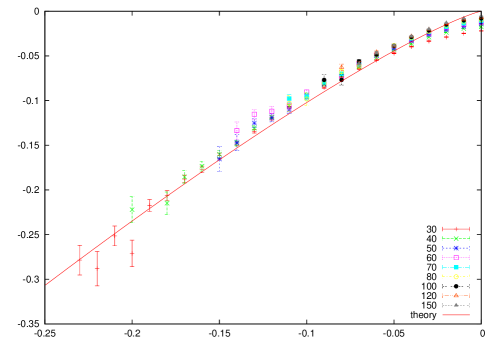
Figure 3: Comparison between the numerical and analytical sample complexity at zero temperature, see text. The data are those of Ref. CMPP .

From the Padé approximants of $c_{5}\beta^{-5}$ and $c_{7}\beta^{-7}$ we estimate $c_{5}\simeq-0.0060(1)\,\beta^{5}$ near $T=0$ and $c_{7}\simeq-0.0150(5)\beta^{7}$ in the SK model. The zero temperature complexity then reads:

$$\Delta\Sigma=-1.62(1)\,|\Delta e|^{6/5}+3.1(1)\,|\Delta e|^{8/5}+O(\Delta e^{8/5})\ ,$$ (13)

Unfortunately the second term yields a big correction to the first one, indeed: i) the exponents of the series grow slowly (as $(6+i)/5$, $i=0,2,3,\dots$ because there is no $n^{6}$ term in $\Phi(n)$) and ii) the coefficients of the series grow quickly with order, actually we expect the series to be asymptotic as is usually the case in this context CR .

In order to bypass this problem and have a good control on $\Delta\Sigma(\Delta e)$ we have adopted a method introduced in CR to obtain $q(x,\tau)$ from its series in powers of $x$ and $\tau$. We have transformed the series of $\Delta\Sigma(\Delta f)$ in powers of $\Delta f$ and $\tau$ in a power series of just $\tau$ by setting $\Delta f=({2\over 45}s^{5}+{1\over 4}\tau^{7})c$ with $c$ a parameter in the range $[0,1]$. The corresponding series in powers of $\tau$ were resummed for any given $c$ through Padé approximants obtaining the curve $\Delta\Sigma(\Delta e)$ in parametric form. By resumming the series of $\Phi(n,\tau)$ as a function of $\tau$ we have been able to obtain the sample complexity in the whole low-temperature phase using the technique of Padé approximants: 18 orders of the Taylor expansion give us a very good control on the function.

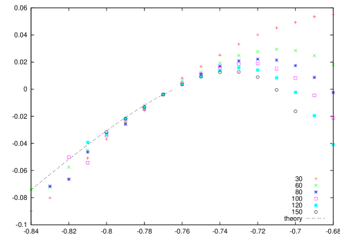
Figure 4: Plot of the numerical complexity (from CMPP ) as a function of the energy density for different sample sizes at zero temperature. The data have been shifted vertically by an amount $\Delta_{N}$ so that the complexity vanishes at the typical energy $E_{typ}=-.7633$.

Using this technique we find that, for not too large $\Delta e$, the zero temperature result shown in fig. (3) differs by less than $1\%$ from the first term of eq.(13) in this range of energy differences. We compared the sample complexity with the numerical data at zero temperature of Ref. CMPP as a function $\Delta e$ and find a very good agreement. For each $N$ we have plotted $\Delta\Sigma_{N}=\ln(P(\Delta e_{N})/N^{5/6})/N$ with $\Delta e_{N}=e-e_{N}$ (the average energy at size $N$): we put the $N^{5/6}$ factor in the definition so that that $\Delta\Sigma$ goes to a constant for $\Delta e_{N}=0$. Unfortunately the dependence of $e_{N}$ on the size is not negligible and the reader may wonder what happens if we plot the data at fixed energy. This has been done in fig.(4), where data (from CMPP ) have been shifted vertically by an amount $\Delta_{N}$ so that the complexity vanishes at the typical energy $E_{typ}=-.7633$, as it should do in the infinite volume limit. This correction ($\Delta_{N}$) goes to zero at large $N$ but it is important for having a good scaling for finite $N$. It is interesting to note that for $E<E_{typ}$ the numerical data approach the theoretical prediction from below, thus strongly suggesting that $\Delta\Sigma(\Delta e)$ is finite at variance with the alternative scenario where $\Delta\Sigma$ goes to $-\infty$ when $N$ goes to infinity.

Using the standard hierarchical ansatz we have computed the large deviations function at all temperatures. In this way we have been able to confirm that the sample complexity $\Delta\Sigma(\Delta f)$ is proportional to $|\Delta f|^{6/5}$ for small negative $\Delta f$, this result strongly suggests that the sample-to-sample fluctuations are proportional to $N^{-5/6}$. We have verified that the numerical data of CMPP are in remarkably good agreement with our absolute prediction. We believe that our results solves the problem of computing the large deviations function for negative $\Delta f$. One could therefore start to study more difficult problems, like the large deviation function for positive $\Delta f$ in the SK model. One could also try to extend our results to other models, such as Bethe lattices or large dimensions short range models, work is in progress in these directions PRprep .

Aknowledgements - We thank the Authors of Ref. CMPP for giving us their numerical data.

Appendix A Power Series of $\Phi(n)$

In this appendix we report the power series of $\Phi(n)$ of the SK model in the low temperature phase up to the 18th order in $n$ and $\tau=1-T$. At all order in $\tau$ the smallest power of $n$ is $n^{5}$ and there is no $n^{6}$ term.

$$\Phi(n) = -\frac{1}{4}-\ln 2-\frac{\tau}{4}+\tau\ln 2-\frac{{\tau}^{2}}{4}-\frac{{\tau}^{3}}{12}+\frac{{\tau}^{4}}{24}-\frac{{\tau}^{5}}{120}+\frac{3\,{\tau}^{6}}{20}-\frac{79\,{\tau}^{7}}{140}+\frac{1679\,{\tau}^{8}}{560}-\frac{13679\,{\tau}^{9}}{720}+\frac{1728361\,{\tau}^{10}}{12600}+$$ (14)

$$-\frac{19214684\,{\tau}^{11}}{17325}+\frac{2741593487\,{\tau}^{12}}{277200}-\frac{3939806687\,{\tau}^{13}}{40950}+\frac{773933492429\,{\tau}^{14}}{764400}-\frac{86662083146207\,{\tau}^{15}}{7567560}+$$

$$+\frac{139738065304401461\,{\tau}^{16}}{1009008000}-\frac{45875375549246420713\,{\tau}^{17}}{25729704000}+\frac{11276190176083149262457\,{\tau}^{18}}{463134672000}+$$

$$n^{5} \left(-\frac{9}{5120}-\frac{99\,\tau}{5120}-\frac{27\,{\tau}^{2}}{320}-\frac{279\,{\tau}^{3}}{1280}-\frac{981\,{\tau}^{4}}{2560}-\frac{351\,{\tau}^{5}}{400}+\frac{2799\,{\tau}^{6}}{12800}-\frac{344241\,{\tau}^{7}}{22400}+\frac{47010861\,{\tau}^{8}}{358400}+\right.$$

$$\left.-\frac{36684189\,{\tau}^{9}}{25600}+\frac{830566899\,{\tau}^{10}}{51200}-\frac{1928757352257\,{\tau}^{11}}{9856000}+\frac{98506298782713\,{\tau}^{12}}{39424000}-\frac{8635947355938261\,{\tau}^{13}}{256256000}\right)+$$

$$n^{7} \left(\frac{81}{143360}-\frac{2673\,\tau}{143360}-\frac{7047\,{\tau}^{2}}{35840}-\frac{35559\,{\tau}^{3}}{35840}-\frac{75573\,{\tau}^{4}}{35840}-\frac{1943757\,{\tau}^{5}}{179200}+\frac{7442847\,{\tau}^{6}}{179200}+\right.$$

$$\left.-\frac{762113853\,{\tau}^{7}}{1254400}+\frac{17011569051\,{\tau}^{8}}{2508800}-\frac{210723811119\,{\tau}^{9}}{2508800}+\frac{13663823711841\,{\tau}^{10}}{12544000}-\frac{1027400967213903\,{\tau}^{11}}{68992000}\right)+$$

$$n^{8} \left(\frac{243}{32768}+\frac{4131\,\tau}{32768}+\frac{15309\,{\tau}^{2}}{16384}+\frac{34263\,{\tau}^{3}}{8192}+\frac{429381\,{\tau}^{4}}{32768}+\frac{2740311\,{\tau}^{5}}{81920}+\frac{11253573\,{\tau}^{6}}{163840}+\right.$$

$$\left.+\frac{107945217\,{\tau}^{7}}{573440}-\frac{669127959\,{\tau}^{8}}{4587520}+\frac{12126319893\,{\tau}^{9}}{2293760}-\frac{183401224893\,{\tau}^{10}}{3276800}\right)+$$

$$n^{9} \left(-\frac{60021}{5734400}-\frac{1720683\,\tau}{5734400}-\frac{3703563\,{\tau}^{2}}{1433600}-\frac{48430143\,{\tau}^{3}}{2867200}-\frac{213993819\,{\tau}^{4}}{5734400}-\frac{2813451327\,{\tau}^{5}}{7168000}+\right.$$

$$\left.+\frac{2765750427\,{\tau}^{6}}{1146880}-\frac{1836578874951\,{\tau}^{7}}{50176000}+\frac{379740674928681\,{\tau}^{8}}{802816000}-\frac{189083279254923\,{\tau}^{9}}{28672000}\right)+$$

$$n^{10} \left(\frac{155277}{3276800}+\frac{911979\,\tau}{819200}+\frac{36721917\,{\tau}^{2}}{3276800}+\frac{110699379\,{\tau}^{3}}{1638400}+\frac{1837467099\,{\tau}^{4}}{6553600}+\frac{2973858543\,{\tau}^{5}}{3276800}+\right.$$

$$\left.+\frac{76627955097\,{\tau}^{6}}{32768000}+\frac{104357662929\,{\tau}^{7}}{16384000}+\frac{853398339489\,{\tau}^{8}}{131072000}\right)+$$

$$n^{11} \left(-\frac{829433601}{5046272000}-\frac{22603330989\,\tau}{5046272000}-\frac{7219643481\,{\tau}^{2}}{180224000}-\frac{20133254457\,{\tau}^{3}}{57344000}-\frac{1149209550873\,{\tau}^{4}}{2523136000}+\right.$$

$$\left.-\frac{218994700592277\,{\tau}^{5}}{12615680000}+\frac{1073108844538299\,{\tau}^{6}}{6307840000}-\frac{61281594304289307\,{\tau}^{7}}{22077440000}\right)+$$

$$n^{12} \left(\frac{131410269}{183500800}+\frac{2903445891\,\tau}{183500800}+\frac{4533651\,{\tau}^{2}}{25600}+\frac{22510325169\,{\tau}^{3}}{18350080}+\right.$$

$$\left.+\frac{1165811276367\,{\tau}^{4}}{183500800}+\frac{5189828163921\,{\tau}^{5}}{229376000}+\frac{89579196304317\,{\tau}^{6}}{917504000}\right)+$$

$$n^{13} \left(-\frac{15299148393873}{5651824640000}-\frac{14089860473859\,\tau}{209924915200}-\frac{330886579531671\,{\tau}^{2}}{565182464000}-\frac{13990469422488399\,{\tau}^{3}}{1836843008000}+\right.$$

$$\left.+\frac{20015370592779843\,{\tau}^{4}}{1335885824000}-\frac{9384066047520578313\,{\tau}^{5}}{10496245760000}\right)+$$

$$n^{14} \left(\frac{66042560169}{5138022400}+\frac{580058908857\,\tau}{2569011200}+\frac{15101741931291\,{\tau}^{2}}{5138022400}+\right.$$

$$\left.+\frac{125170590832281\,{\tau}^{3}}{6422528000}+\frac{7885818877083003\,{\tau}^{4}}{51380224000}\right)+$$

$$n^{15} \left(-\frac{1557529661529486369}{29389488128000000}-\frac{13663672258178594727\,\tau}{14694744064000000}-\frac{107529809054090820291\,{\tau}^{2}}{14694744064000000}+\right.$$

$$\left.-\frac{46100805957050412573\,{\tau}^{3}}{262406144000000}\right)+$$

$$n^{16} \left(\frac{190687314873528513}{723433553920000}+\frac{320621966627776497\,\tau}{180858388480000}+\frac{18912071856450181023\,{\tau}^{2}}{361716776960000}\right)+$$

$$n^{17} \left(-\frac{126373462658844234883011}{111915170791424000000}-\frac{92659942781039607442731\,\tau}{55957585395712000000}\right)+$$

$$n^{18} \frac{10254234479592769713}{1808583884800000}$$

References

• (1) I. Kondor, J. Phys. A 16 L127 (1983)
• (2) A. Crisanti, G. Paladin, H.-J. Sommers and A. Vulpiani, J. PHys. I France 2, 1325 (1992)
• (3) S. Boettcher, Europhys. Lett. 67, 453 (2004)
• (4) J.-P. Bouchaud, F. Krzakala and O. C. Martin, Phys. Rev. B 68, 224404 (2003).
• (5) A. Andreanov, F. Barbieri and O. C. Martin, Eur. Phys. J. B. 41 (3), 365 (2004)
• (6) M. Palassini, cond-mat/0307713
• (7) S. Boettcher, Eur. Phys. J. B 46, 501 (2005)
• (8) H. G. Katzgraber, M. Korner, F. Liers, M. Junger and A. K. Hartmann, Phys. Rev. B 72, 094421 (2005)
• (9) K. F. Pal, Physica A 367, 261 (2006)
• (10) T. Aspelmeier and M.A. Moore, Phys. Rev. Lett. 90, 177201 (2003).
• (11) C. De Dominicis and P. Di Francesco, cond-mat/0301066.
• (12) M. Mezard, G. Parisi and M. A. Virasoro, Spin Glass Theory and Beyond (World Scientific, Singapore, 1987)
• (13) B. Derrida, Phys. Rev. B 24 2613 (1981).
• (14) M. Talagrand Large deviations, Guerra’s and A.S.S. Schemes, and the Parisi hypothesis, to appear in the proceedings of the conference Mathematical Physics of Spin-Glasses, Cortona (2005).
• (15) A. Crisanti and T. Rizzo, Phys. Rev. E 65, 046137 (2002)
• (16) H. J. Sommers, W. Dupont, J. Phys. C 17 (1984) 5785-5793.
• (17) Vik. Dotsenko, S. Franz and M. Mezard, J. Phys. A. Math. Gen. 27 (1994) 2351-2365.
• (18) G. Parisi and T. Rizzo, in preparation.
• (19) A. Crisanti, T. Rizzo and T. Temesvari, Eur. Phys. J. B 33, 203-207 (2003).