Non adiabatic quantum search algorithms

Abstract

We present two new continuous time quantum search algorithms similar to the adiabatic search algorithm, but now without an adiabatic evolution. We find that both algorithms work for a wide range of values of the parameters of the Hamiltonian, and one of them has, as an additional feature that, for values of time larger than a characteristic one, it will converge to a state which can be close to the searched state.

I Introduction

Quantum computation has attracted the attention of researchers from several different areas Chuang . This field of knowledge presents new scientific challenges to learn how to work with quantum properties to obtain more efficient algorithms. However, relatively few quantum algorithms were created; among them, Shor’s and Grover’s Shor ; Grover algorithms are the best known. Grover’s search algorithm locates a marked item in an unsorted list of $N$ elements in a number of steps proportional to $\sqrt{N}$, instead of $O(N)$ as in the classical case. It performs a unitary transformation of the initial quantum state so as to increase the likelihood that the marked state of interest will be measured at the output (amplification technique). It has been proved that there are neither quantum nor classical algorithms that can perform faster such an unstructured search Boyer . This search algorithm has also a continuous time version Farhi that has been described as the analogue of the original Grover algorithm. From this continuous time version, and using the quantum adiabatic theorem, adiabatic search algorithms have been developed Farhi2 ; Farhi3 ; Roland , that consist in guessing a time-dependent Hamiltonian whose dynamics evolves slowly enough so that it remains always near its instantaneous ground state. They solve the search problem in a time proportional to $\sqrt{N}/\delta$, where $\delta$ is a precision parameter that depends on the energy difference between the two lowest states.

Another way to generate a continuous time quantum search algorithm alejo has been recently developed, that finds a discrete eigenstate of a given Hamiltonian $H_{0}$. This algorithm behaves like Grovers’s, and explicitly shows that the search algorithm is essentially a resonance phenomenon between the initial and the searched states Grover2 .

In this work we present two new continuous time search algorithms that are controlled by a time dependent Hamiltonian, similarly to the case of the quantum adiabatic search algorithm, but now the evolution is non adiabatic; then it is not necessary to impose slowness to the dynamics in order to preserve the system in the fundamental state. These algorithms provide new insights to search algorithms, in particular: a connection between the resonant and the adiabatic search algorithms (for the first case), or the possibility to generate a new type of search algorithm in which one does not need to pick up a particular instant of time when the measure has to be performed (for the second case), provided the parameters characterizing the Hamiltonian are conveniently chosen. In this second case, one reaches an asymptotic form for the searching probability, which is rather independent on the size of the database $N$, at the cost of increasing the energy resources in the Hamiltonian as $N$ grows.

The paper is organized as follows. In the next two sections we develop the two models of non adiabatic algorithms. In the last section we draw the conclusions of this work.

II Non adiabatic algorithm I

Consider $N$ items in the database, each associated with a vector in the complete orthonormal set $\left\{|n\rangle,\text{ }n=1,2,...,N\right\}$ in a Hilbert space. Let us call $|s\rangle$ the unknown searched state that is associated with the marked item belonging to the previous group. We assume that the initial state is the symmetric normalized state

$$\left|\psi_{0}\right\rangle=\frac{1}{\sqrt{N}}\sum\limits_{n=1}^{N}|n\rangle,$$ (1)

and define the two Hamiltonians

$$H_{0}=I-\left|\psi_{0}\right\rangle\left\langle\psi_{0}\right|,$$ (2)

$$H_{s}=I-\left|s\right\rangle\left\langle s\right|,$$ (3)

where $I$ is the identity matrix, their ground states being $\left|\psi_{0}\right\rangle$ and $\left|s\right\rangle$ respectively. The algorithm is built on the following time-dependent Hamiltonian

$$H(t)=f(t)H_{0}+g(t)H_{s}\,,$$ (4)

where $f(t)$ and $g(t)$ are time dependent functions that will be defined later. Notice that $H_{s}$ plays the equivalent role to ’marking’ the searched state in Grover’s algorithm. The goal of the search algorithm is to change $\left|\psi_{0}\right\rangle$ into $|s\rangle$ or some approximation there of, following the dynamics generated by the Schrödinger equation. In this problem, we can restrict the analysis to the two-dimensional space spanned by $|s\rangle$ and $|p\rangle=$ $\frac{1}{\sqrt{N-1}}\sum\limits_{n=1,n\neq s}^{N}|n\rangle$. The wave function is then expressed as

$$\left|\psi(t)\right\rangle=a_{s}(t)|s\rangle+a_{p}(t)|p\rangle\,,$$ (5)

for some $a_{s}(t)$, $a_{p}(t)$ such that  $\left|a_{s}(t)\right|^{2}+\left|a_{p}(t)\right|^{2}=1$ with $a_{s}(0)=\sqrt{1/N}$ and $a_{p}(0)=\sqrt{1-1/N}$. In the $\{|s\rangle$, $|p\rangle\}$ basis we have the following matrix for the Hamiltonian

$$H(t)=\frac{1}{N}\left[\begin{array}[]{cc}\left(N-1\right)f(t)&-\sqrt{N-1}f(t)\\ -\sqrt{N-1}f(t)&\text{ \ \ \ }f(t)+Ng(t)\end{array}\right].$$ (6)

The above matrix can be rewritten under the form

$$H(t)=\frac{1}{2}(f+g)I+\frac{1}{2}\omega(t)\vec{n}\cdot\vec{\sigma}$$ (7)

where $\omega(t)=\sqrt{(f-g)^{2}+4fg/N}$, $\vec{n}=\frac{1}{\omega(t)}(-2\sqrt{N-1}f/N,0,f-g-2f/N)$ is an unitary vector and $\vec{\sigma}$ stands for the Pauli matrices. Defining $\vec{n}=(\sin\theta,0,\cos\theta)$, one can easily obtain the functions $f$ and $g$ as a function of $\theta$, with the following result:

$$f(t) = -\frac{N}{2\sqrt{N-1}}\omega(t)\sin\theta$$ (8)

$$g(t) = -\frac{N}{2\sqrt{N-1}}\omega(t)\cos(\theta+\beta)$$ (9)

with $\sin\beta\equiv(2-N)/N$, $\cos\beta\equiv 2\sqrt{N-1}/N$.

The first term in Eq. (7) is proportional to the identity, and therefore amounts to a common (time dependent) phase that can be ignored if one only wants to evaluate probabilities. We will concentrate on the second term, which has eigenvalues $E_{\pm}(t)=\pm\frac{1}{2}\omega(t)$ with corresponding time-dependent eigenvectors $|E_{+},t>=(\cos\frac{\theta}{2},\sin\frac{\theta}{2})$ and $|E_{-},t>=(-\sin\frac{\theta}{2},\cos\frac{\theta}{2})$, with respect to the basis $\{|s\rangle,p\rangle\}$. In this form, it becomes evident that the evolution originated from the Hamiltonian amounts to a (time-dependent) rotation in the space spanned by the states $\{|s\rangle,p\rangle\}$ with the goal of maximizing the probability of the $|s\rangle$ state.

The Schrödinger equation in this basis, in units such that $\hbar=1$, becomes

$$\left[\begin{array}[]{c}\frac{da_{s}(t)}{dt}\\ \frac{da_{p}(t)}{dt}\end{array}\right]=-iH(t)\left[\begin{array}[]{c}a_{s}(t)\\ a_{p}(t)\end{array}\right].$$ (10)

Now we take the following steps: first, we change to a new basis where this Hamiltonian is diagonal; second, we solve the Schrödinger equation in that basis, and third, we return to the original basis, where we are searching the state $|s\rangle$. The wave function, $\left|\psi(t)\right\rangle$ can be expressed as a combination of the time-dependent eigenstates $|E_{+},t\rangle$, $|E_{-},t\rangle,$

$$\left|\psi(t)\right\rangle = a_{+}(t)\exp(-i\int\limits_{0}^{t}E_{+}(t)dt)|E_{+},t\rangle$$ (11)

$$+a_{-}(t)\exp(-i\int\limits_{0}^{t}E_{-}(t)dt)|E_{-},t\rangle.$$

We have two expressions for the wave function, one in the $\{|s\rangle$, $|p\rangle\}$ basis, Eq. (5), and the other one in the $\{|E_{+},t\rangle,|E_{-},t\rangle\}$ basis, Eq. (11). The relation between both basis can be expressed as a relation between its coefficients, that is

$$\left[\begin{array}[]{c}a_{s}(t)\\ a_{p}(t)\end{array}\right]=U^{\dagger}(t)\left[\begin{array}[]{c}a_{+}(t)\exp(-i\int\limits_{0}^{t}E_{+}(t)dt)\\ a_{-}(t)\exp(-i\int\limits_{0}^{t}E_{-}(t)dt)\end{array}\right]\text{,}$$ (12)

where

$$U^{\dagger}(t)=\left(\begin{array}[]{cc}\cos\frac{\theta}{2}&-\sin\frac{\theta}{2}\\ \sin\frac{\theta}{2}&\cos\frac{\theta}{2}\end{array}\right),$$ (13)

The Schrödinger equation in the new coordinates is

$$\left[\begin{array}[]{c}\frac{da_{+}(t)}{dt}\\ \frac{da_{-}(t)}{dt}\end{array}\right]=-M^{\dagger}(t)U(t)\frac{dU^{\dagger}(t)}{dt}M(t)\left[\begin{array}[]{c}a_{+}(t)\\ a_{-}(t)\end{array}\right],$$ (14)

where $M_{11}(t)=\exp(-i\int\limits_{0}^{t}E_{+}(t)dt)$, $M_{22}(t)=\exp(-i\int\limits_{0}^{t}E_{+}(t)dt)$ and $M_{12}(t)=M_{21}(t)=0$. From here, one easily arrives to

$$\frac{da_{+}(t)}{dt} =-\Omega(t)\text{ \ }a_{-}(t),$$ (15)

$$\frac{da_{-}(t)}{dt} =\Omega^{\ast}(t)\text{ }a_{+}(t),$$ (16)

where

$$\Omega(t)\equiv-\frac{1}{2}\dot{\theta}\exp(i\int\limits_{0}^{t}\omega(t)dt),$$ (17)

with $\dot{\theta}=\frac{d\theta}{dt}$. Alternatively, we can rewrite Eq. (17) as

$$\Omega(t) = \frac{\sqrt{N-1}}{N\omega{{}^{2}}}\left(\frac{dg(t)}{dt}f(t)-g(t)\frac{df(t)}{dt}\right)$$ (18)

$$\times \exp(i\int\limits_{0}^{t}\omega(t)dt);$$

we shall take $f(0)=1$ and $g(0)=0$ in this section, then the initial condition in the new coordinates are $a_{+}(0)=0$ and $a_{-}(0)=1$. Up to this point, our treatment of the problem is similar to that of the adiabatic algorithm. Now to proceed further we shall choose the function $\theta(t)$ (or, equivalently, the functions $f(t)$ and $g(t)$) for the non adiabatic approach that has similarities with the resonant search algorithm. As seen in Eq. (17), if we choose $\theta(t)$ so as to cancel the time dependence of the modulus of $\Omega$, the system Eqs. (15, 16) will have an oscillatory solution between the amplitudes $a_{+}(t)$ and $a_{-}(t)$, with a period proportional to $\sqrt{N}$, which can be identified with the Grover search time. This situation reminds us of the resonant search algorithm alejo , but now these amplitudes are not the amplitudes $a_{s}(t)$ and $a_{p}(t)$.

In order to solve analytically the system Eqs. (15, 16) we shall impose the conditions:

$$\frac{dg(t)}{dt}f(t)-g(t)\frac{df(t)}{dt}\equiv\varepsilon\left(\alpha t+\gamma\right)^{2},$$ (19)

$$\omega(t)=\left|\alpha t+\gamma\right|.$$ (20)

In these expressions $\varepsilon$ is a coupling parameter between the states $a_{+}(t)$ and $a_{-}(t)$, $\alpha$ is the velocity parameter associated to the energy gap and $\gamma=1$ is dictated by our choice of $f(0)$ and $g(0)$. One can check that Eqs. (19,20) are equivalent to imposing

$$\dot{\theta}=2\Omega_{0}$$ (21)

with $\Omega_{0}$ a constant, which we rewrite as $\Omega_{0}=\frac{\sqrt{N-1}}{N}\varepsilon$. In this way conditions (19,20) simply imply both a mixing angle $\theta$(t) and a gap $\omega(t)$ which evolve linearly with time, and thus determine the time evolution of functions $f(t)$ and $g(t)$, see Eqs. (8,9).

We can decouple Eqs. (15, 16) to obtain a differential equations for $a_{{-}}(t)$ (and similarly for $a_{{+}}(t)$)

$$\frac{d^{2}a_{-}}{dt^{2}}+i\omega(t)\frac{da_{-}}{dt}+\Omega_{0}{}^{2}a_{-}=0.$$ (22)

This equation can be solved in the same way as was done in Zener . The change of variable

$$W=\exp\left[\frac{i}{4}(\alpha t^{2}+2\gamma t)\right]a_{-},$$ (23)

leads to

$$\frac{d^{2}W}{dz^{2}}+\left(\eta+\frac{1}{2}-\frac{1}{4}z^{2}\right)W=0,$$ (24)

where

$$z=\sqrt{\alpha}\exp(-i\pi/4)(t+\gamma/\alpha)$$ (25)

and

$$\eta=i\frac{\Omega_{0}^{2}}{\alpha}.$$ (26)

The solutions of the Eqs. (24) are the parabolic cylinder function $D_{\eta}(z)$ Gradshteyn . In our case the general solution is

$$W(z)=A_{1}D_{\eta}(z)+A_{2}D_{\eta}(-z),$$ (27)

where the coefficients are determined by the initial conditions $a_{-}(0)=1$, and $\frac{da_{-}(0)}{dt}=0$. These coefficients are

$$A_{1}=\frac{D_{\eta-1}(-z_{0})}{D_{\eta-1}(z_{0})D_{\eta}(-z_{0})+D_{\eta}(z_{0})D_{\eta-1}(-z_{0})},$$ (28)

$$A_{2}=\frac{D_{\eta-1}(z_{0})}{D_{\eta-1}(z_{0})D_{\eta}(-z_{0})+D_{\eta}(z_{0})D_{\eta-1}(-z_{0})}.$$ (29)

Finally, the amplitude $a_{+}(t)$ can be calculated using the above result for $a_{-}(t)$ and Eq. (16).

Let us discuss in more detail the qualitative behavior of the results we have obtained so far. For large $N$ and finite $\varepsilon$ in such a way that $\Omega_{0}\simeq\frac{\varepsilon}{\sqrt{N}}\ll 1$ it follows from the Eqs. (23, 25, 26, 27, 28, 29) that $\left|a_{{-}}(t)\right|\simeq 1$, $\left|a_{{+}}(t)\right|\simeq 0$. On the other hand, for large $N$ one can approximate $\theta\simeq 2\Omega_{0}t$. Then using Eq. (12), the following approximation for the probabilities of the searched and the orthogonal states are obtained

$$P_{s}(t)\simeq\sin^{2}(\Omega_{0}t),$$ (30)

$$P_{p}(t)\simeq\cos^{2}(\Omega_{0}t),$$ (31)

which are valid whenever $t$ satisfies $(\alpha t+\gamma)>0$. Note that the Eqs. (30, 31) are independent of the value of $\alpha$ if the previous conditions are verified. Then, if we let the system evolve during a time $\tau\equiv\frac{\pi\sqrt{N}}{2\varepsilon}$, and we measure immediately after that, the probability to obtain the searched state is equal to one. In this case our method behaves qualitatively like Grover’s. The parameter $\varepsilon$ allows us for a faster search (relatively to the standard Grover’s algorithms): one can even obtain a characteristic time $\tau\sim 1$. This speedup is allowed because the energy scale in the Hamiltonian, defined by the functions $f(t)$ and $g(t)$ is large enough (c.f. Eq. (22) in Das ), provided that $\Omega_{0}\ll 1$. For concreteness, we will adopt the value $\varepsilon=1$. Additionally we have recovered our interpretation of the search algorithm as a quantum resonance between states alejo ; alejo1 ; alejo2 ; alejo3 ; now the resonance is between the searched and the orthogonal states.

The above result shows that the non adiabatic algorithm works correctly for $\alpha>0$ (remember that $\gamma=1$). We have verified this situation for several values of $N$ and $\alpha>0$ using the exact equation in Fig. 1. The figure shows a periodic behavior with the Grover characteristic time and the correctness of the approximation in Eqs. (30, 31) as $N$ increases.

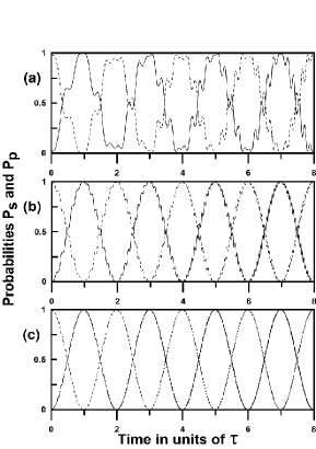
Figure 1: Probabilities as a function of time in units of the characteristics time $\tau\equiv\frac{\pi\sqrt{N}}{2\varepsilon}$. The the full line corresponds to the searched state $P_{s}$, the dashed line to the orthogonal state $P_{p}$. In all cases $\alpha>0$, but the probabilities are independent of the value of $\alpha$. The sizes of the searched set are: (a) $N=50$, (b) $N=500$, (c) $N=5000.$

When $\alpha=0$ (see Eq. (22)) $a_{-}$ and $a_{+}$ can be easily obtained analytically

$$a_{-}(t) = \exp(-i\frac{\gamma}{2}t)\biggl{[}\cos\phi(t)$$ (32)

$$+ \frac{i\gamma}{\sqrt{\left(\frac{\gamma}{2}\right)^{2}+\Omega_{0}^{2}}}\sin\phi(t)\biggr{]}$$

$$a_{+}(t)=\frac{\Omega_{0}\exp(-i\frac{3\gamma}{2}t)}{\sqrt{\left(\frac{\gamma}{2}\right)^{2}+\Omega_{0}^{2}}}\sin\phi(t)$$ (33)

with $\phi(t)=\sqrt{\left(\frac{\gamma}{2}\right)^{2}+\Omega_{0}^{2}}t$. From these expressions, and for large $N$, $\Omega_{0}\ll 1$, $\left|a_{+}(t)\right|\simeq 0$, $\left|a_{-}(t)\right|\simeq 1$ and using the same arguments as before, it can be shown that the search algorithm also works in this case. For $\alpha<0$ the behavior of the system is quite more complex. If, additionally, $\left|\alpha\right|\simeq 0$ (then both $\left|z_{0}\right|$ and $\left|z\right|$ go to infinity) using Eqs. (25, 27, 28, 29, 12) and the asymptotic property of the parabolic cylinder functions, it can be shown that $P_{-}(t)=\left|a_{-}(t)\right|^{2}\simeq 1$ as before, then for large $N$ and $\Omega_{0}<1$ Eqs. (30, 31) are again obtained, and the search algorithm continues to operate. For the case $\alpha<0$ but finite we shall use another reasoning that could have also be used in the previous cases. Notice that the characteristic frequencies of the probability amplitudes ($\sim\Omega_{0}$) are, in general, very small compared with the time-dependent characteristic frequency of $\Omega(t)$ i.e. $\frac{1}{t}\int\limits_{0}^{t}\omega(t)dt$, then the stationary phase method can be used to integrate approximately the differential equations Eqs. (15, 16) for $\alpha\neq 0$. We have used this method in the case $\alpha<0$ and $\alpha$ finite, to obtain Eqs. (30, 31) with the condition $t<t_{c}\equiv-\frac{\gamma}{\alpha}$. The time $t_{c}$ is the ‘close approach time’, defined as the time when the derivative of the phase of $\Omega(t)$ vanishes (see Eq. (17)) and at the same time the energy levels cross each other. Then the search algorithm operates up to this time if $\Omega_{0}\ll\frac{1}{t}\int\limits_{0}^{t}\omega(t)dt$. Fig. 2 was obtained using the exact results of this paper. It shows the probability $P_{s}$ for several values of $\alpha$, and also that the approximation made in Eqs. (30, 31) remains valid for times $t<t_{c}$. For times $t\geq$ $t_{c}$ our previous argument cannot be applied, and the periodicity of the behavior is not clear because other frequencies are present. This figure establishes that, as $\left|\alpha\right|\$is decreased, the close approach time $t_{c}$ increases; in the limit, the algorithm works for all times.

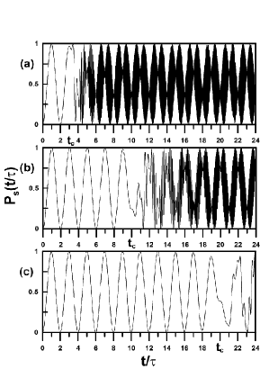
Figure 2: Probability of the searched state $P_{s}$ as a function of time. $N=5000$, in (a) $\alpha=-0.31\gamma/\tau$, in (b) $\alpha=-0.10\gamma/\tau$ in (c) $\alpha=-0.05\gamma/\tau$. Note that the values $t_{c}$ change inversely with $\alpha$.

To close this section, let us remark that the previous results can also be obtained without the use of the mobile base in the following way: Let us substitute the expressions of $f(t)$ and $g(t)$ given by the Eqs. (8,9) in the equations Eq. (10). These equations, together with the normalization of the wave function and the conditions of maximization of the amplitude of the searched state, allow to find the time for which the probability of the search state is maximum. The maximization conditions are $\left|\frac{da_{s}(t)}{dt}\right|=0$ y $\left|a_{s}(t)\right|=1$ and, as a result, we obtain that they are satisfied for those values of $\tau$ such that

$$f(\tau)=\frac{N\left(\alpha\tau+\gamma\right)}{2\sqrt{N-1}}\cos\left(2\Omega_{0}\tau+\beta\right)=0\text{.}$$ (34)

From this equation it is deduced that, if $\alpha\tau+\gamma\neq 0$ then

$$\tau=\frac{\pi N}{2\sqrt{N-1}\epsilon}l\text{,}$$ (35)

with $l=1,2,3,...$. As a result, we see that the algorithm works in an equivalent way to the Grover algorithm for all times, if $\alpha$ is positive, and only until the close approach time if $\alpha$ is negative.

III Non adiabatic algorithm II

In this section we introduce a new idea for the searching Hamiltonian which is based on a different choice of the functions $f(t)$ and $g(t)$ and possesses the characteristic that one does not need to single out a given time in order to find the searched state with a high probability, provided the parameters of the Hamiltonian are chosen appropriately.

Let us return to Eq. (6) and choose now $f(t)=\frac{N}{\sqrt{N-1}}$, then we have:

$$H(t)=\sqrt{N-1}I+\left[\begin{array}[]{cc}0&-1\\ -1&\text{ \ \ \ }g(t)+\frac{2-N}{\sqrt{N-1}}\end{array}\right].$$ (36)

The first term in this expression is constant and proportional to the identity. One can, as done in the previous section, ignore it for the sake of solving the Schrödinger equation. Let us choose the (2,2) matrix element in Eq. (36) so that it changes linearly with time. In this way, the resulting Hamiltonian (in the fixed basis) mimics the evolution of the functions $a_{+}(t)$ and $a_{-}(t)$ obtained in Section 2. To be more precise, we choose

$$g(t)=\frac{N-2}{\sqrt{N-1}}+2(b-at),$$ (37)

with $a$ and $b$ constants. Notice that $f(t)$ and $g(t)$ scale with $N$ in the same way as in the previous section, therefore the same discussion regarding the energy cost will apply. In this second model, the gap energy function takes the simple form $\omega(t)=\sqrt{(at-b)^{2}+1}$.

With the above definitions, apart from a global phase which we will ignore, the Hamiltonian Eq. (36) gives rise to the same evolution as the matrix

$$H^{\prime}(t)=\left[\begin{array}[]{cc}0&-1\\ -1&2b-2at\end{array}\right].$$ (38)

We will allow time to run from $t=0$ to arbitrarily large values ($t\rightarrow\infty)$. As we observe, the above Hamiltonian bears a close resemblance to the usual ones introduced in adiabatic quantum computations, in the sense that it has a time variation which is linear in time. However, in our case we will not start from the ground state of the Hamiltonian, and we will not intend either to force the system to be driven to its ground state for some finite time $T$ by making use of the adiabatic theorem.

The resulting evolution equations for $a_{s}(t)$ and $a_{p}(t)$ can be easily decoupled, leading to

$$\frac{d^{2}a_{s}}{dt^{2}}+2i(b-at)\frac{da_{s}}{dt}+a_{s}=0$$ (39)

This equation has to be supplemented by the initial conditions $a_{s}(0)=\sqrt{1/N}$, $\frac{da_{s}}{dt}(t=0)=ia_{p}(0)=i\sqrt{(N-1)/N}$. With the substitution

$$W=a_{s}\exp[-i(\frac{1}{2}at^{2}-bt)]$$ (40)

we arrive to the same equation as in Eq. (24), but now $z=\sqrt{2ai}(t-b/a)$ and $\eta=-\frac{i}{2a}$. The solution to this equation can still be written in the form (27), with coefficients $A_{1}$ and $A_{2}$ which have to be determined from the initial conditions. After some algebra, we arrive to

$$A_{1}=\frac{1}{\sqrt{N}}\frac{D_{\eta-1}(-z_{0})+\sqrt{N}q_{0}D_{\eta}(-z_{0})}{D_{\eta-1}(z_{0})D_{\eta}(-z_{0})+D_{\eta}(z_{0})D_{\eta-1}(-z_{0})}$$ (41)

$$A_{2}=\frac{1}{\sqrt{N}}\frac{D_{\eta-1}(z_{0})-\sqrt{N}q_{0}D_{\eta}(z_{0})}{D_{\eta-1}(z_{0})D_{\eta}(-z_{0})+D_{\eta}(z_{0})D_{\eta-1}(-z_{0})},$$ (42)

where $q_{0}=\sqrt{2a}\sqrt{\frac{N-1}{N}}\exp(i3\pi/4)$ and $z_{0}=-b\sqrt{\frac{2}{a}}\exp(i\pi/4)$. In order to give a result for the searched probability $P_{s}(t)=|a_{s}(t)|^{2}$, we need to particularize the values of $N$, $a$ and $b$. Using the asymptotic form for the parabolic cylinder functions Gradshteyn , one can obtain the following result for the limit $\lim_{t\rightarrow\infty}P_{s}(t)$:

$$p(a,b)=\lim_{t\rightarrow\infty}P_{s}(t)=|A_{1}e^{k\pi/4}+A_{2}e^{-3\pi k/4}|^{2},$$ (43)

with $k=\frac{1}{2a}$.

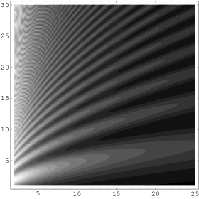
Figure 3: Contour plot for the limiting probability $p(a,b)$ when $N=100$. The horizontal axis corresponds to $a$, and the vertical axis to $b$. Brighter regions represent a higher probability, while dark regions indicate a probability close to zero.

Fig. 3 shows a contour plot of the limiting values of the probability $p(a,b)$ with $N=100$. As readily seen, it reveals a complicated pattern with bands of high probability and low-probability valleys. These patterns depend quite weakly on $N$ and, in fact, it is possible to obtain the limit $N\rightarrow\infty$ in Eqs. (42). Fig. 4 corresponds to this limit. As can be seen, the changes are moderate, showing that the asymptotic probability saturates for large values of $N$.

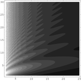
Figure 4: Same as Fig. 3, for the asymptotic $N\rightarrow\infty$ limit.

In order to explicitly show the differences between our proposal and the adiabatic treatment, we have calculated the probability $P_{s}(t)$ for different parameters. The results are shown in Fig. 5. Given the structure seen in Fig. 4, we choose a fixed $b=4.5$, and plot the probability for three values of $a$: 1, 5 and 20. The value of $N$ we used is $=10^{6}$ which, according to the previous discussion, is equivalent to taking $N\rightarrow\infty$.

In this figure, it is apparent that a transition occurs at the time $t_{c}=b/a$, corresponding to the minimum distance between the two eigenvalues of the Hamiltonian. The asymptotic behavior with time is clear from this figure, although the final probability strongly depends on the particular choice of $a$ and $b$, as seen before. It is important to note that the corresponding Grover time would be of the order $\sqrt{N}\sim 10^{3}$, which represents a much larger time scale than the one showed in this figure.

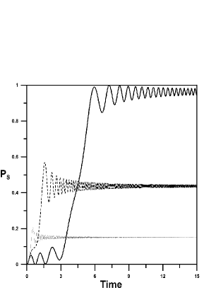
Figure 5: Evolution of the probability for the searched state $P_{s}$ as a function of time, for a fixed $b=4.5$ and three values of the parameter $a$: 1 (solid line), 5 (thick dashes) and 20 (thin dashes).

Therefore, our proposal consists on implementing the Hamiltonian 6 but with the functions $f$ and $g$ as defined above. By an appropriate choice of the parameters $a$ and $b$ appearing in $g(t)$, one can make the probability of the searched state to reach a value close to unity within a scale of time which is much shorter (for large $N$) than the corresponding Grover’s time. At first sight, this appears to be in contradiction with the well-known result that Grover’s algorithm is optimal for quantum searching Boyer . However, it has been discussed that adiabatic search can be done at a shorter time (even with a time scale which is independent of $N$) at the expense of increasing the energy resources Das ; Wei . This, in fact, seems to be the case within our proposal, if one remembers that, in order to obtain the Hamiltonian 36 using the resources defined in 6, the functions $f$ and $g$ will scale as $\sqrt{N}$, thus increasing the energy resources as $N$ grows.

IV Conclusions

We have developed two new continuous time quantum search algorithms using a time-dependent Hamiltonians in a non adiabatic regime. Our approach differs from to the usual (adiabatic) approach, when one starts from the initial ground state and tries to evolve slowly, making use of the adiabatic theorem to stay close to the instantaneous ground state. For the first case, the key of the algorithm is that the derivative of the amplitudes $a_{-}(t)$ and $a_{+}(t)$ have a fast time variation with a vanishing mean value over the characteristic time $\tau$ i.e.$\frac{1}{\tau}\int\limits_{0}^{\tau}\frac{da_{{}_{\pm}}(t)}{dt}dt\sim 0$, then starting from the ground state, in the mobile basis $\left\{|E_{+},t\rangle,|E_{-},t\rangle\right\}$, the system remains near this ground state for all times. This algorithm behaves like the Grover algorithm for non negative values of the parameter $\alpha$, independently of its particular value, for a large $N$ and $\Omega_{0}\lll 1$. The optimal search time is proportional to $\sqrt{N}$, and the probability to find the searched state oscillates periodically. For $\alpha<0$ the algorithm does not work for $t\geq t_{c}$, with $t_{c}$ the close approach time.

The second algorithm makes use of similar resources to build up a Hamiltonian that changes linearly with time. In our proposal, the initial and final states do not correspond to the ground states of the Hamiltonian, and the system is allowed to evolve up to arbitrarily large times, showing a convergence towards a final state after a finite transition time. When the parameters are chosen appropriately, the asymptotic state can overlap with the searched state with high probability, and one does not need to pick up a special value of time to perform the measurement in order to obtain the desired result.

Both algorithms can be used to perform a search within a time which can be made shorter than the standard Grover’s time, at the expense of using also larger than standard energetic resources.

These results open the possibility for the design of new quantum algorithms that perform a search on an unstructured database (and possibly other algorithmic tasks) alternatively to the existing algorithms.

Acknowledgments

We acknowledge the comments made by V. Micenmacher and the support from PEDECIBA and PDT S/C/OP/28/84. This work has also been supported by the Spanish Ministerio de Educación y Ciencia through Projects AYA2004-08067-C01 and FPA2005-00711.

References

- (1) M. Nielssen and I. Chuang, Quantum Computation and Quantum Information, Cambridge University Press, 2000.
- (2) P.W. Shor, Proc. of the 35th Annual Symposium on the Foundations of Computer Science, Ed. S. Goldwasser, Los Alamitos, CA, 1994; ibid. SIAM J. Comp., 26, 1484, (1997).
- (3) L. K. Grover, Proc. 28th STOC, 212, Philadelphia, PA (1996) and L.K. Grover, Phys. Rev. Lett. 79, 325 (1997)
- (4) M. Boyer, G. Brassard, P. Høyer, and A. Tapp, Fortsch. Phys. 46 (1998) 493, arXiv:quant-ph/9605034.
- (5) E. Farhi and S. Gutmann. Phys. Rev. A 57, 2403 (1998)
- (6) A. M. Childs and J. Goldstone Phys. Rev. A 70, 022314 (2004), arXiv:quant-ph/0306054, quant-ph/0405120
- (7) E. Farhi, J. Goldstone, S. Gutmann and M. Sipser, arXiv:quant-ph/0001106
- (8) E. Farhi, J. Goldstone, S. Gutmann and D. Nagaj, arXiv:quant-ph/0512159
- (9) J. Roland and N. J. Cerf Phys. Rev. A 65, 042308-1 (2002)
- (10) A. Romanelli, A. Auyuanet, R. Donangelo. Physica. A, 360, 274. (2006), arXiv:quant-ph/0502161
- (11) L. K. Grover, A.M. Sengupta, Phys. Rev. A 64, 032319 (2002), arXiv:quant-ph/0109123.
- (12) S. Das, R. Kobes and G. Kunstatter, J. Phys. A: Math. Gen. 36 (2003) 2839
- (13) C. Zener, Proc. R. Soc. London, A, 137, 696 (1932)
- (14) I. S. Gradshteyn, I. M. Ryzhik Table of Integrals, Series and Products, Academic Press, (1994)
- (15) A. Romanelli, A. Auyuanet, R. Donangelo. Physica. A, 375, 133. (2007), arXiv:quant-ph/0508142
- (16) A. Romanelli, R. Donangelo, to appear in Physica. A, arXiv:quant-ph/0608019
- (17) A. Romanelli, Physica. A, 379, 545, (2007), arXiv:quant-ph/0609106.
- (18) Zhaohui Wei and Mingsheng Ying, quant-ph/0412117.