The richest superclusters

Abstract

Context. Superclusters are the largest systems in the Universe to give us information about the formation and evolution of structures in the very early Universe. Our present series of papers is devoted to the study of the morphology and internal structure of superclusters of galaxies.

Aims. We study the morphology of the richest superclusters from the catalogues of superclusters of galaxies in the 2dF Galaxy Redshift Survey and compare the morphology of real superclusters with model superclusters in the Millennium Simulation.

Methods. We use Minkowski functionals and shapefinders to quantify the morphology of superclusters: their sizes, shapes, and clumpiness. We generate empirical models of simple geometry to understand which morphologies correspond to the supercluster shapefinders.

Results. Rich superclusters have elongated, filamentary shapes with high-density clumps in their core regions. The clumpiness of superclusters is determined using the fourth Minkowski functional $V_{3}$. In the $K_{1}$-$K_{2}$ shapefinder plane the morphology of superclusters is described by a curve which is characteristic to multi-branching filaments. We also find that the differences between the fourth Minkowski functional $V_{3}$ for the bright and faint galaxies in observed superclusters are larger than in simulated superclusters.

Conclusions. Our results show how the Minkowski functionals and shapefinders describe the morphology of superclusters. We see that the observed superclusters are more diverse than model superclusters. There are a number of differences between observed and model superclusters, especially in the distribution of bright and faint galaxies.

1 Introduction

Superclusters of galaxies with characteristic dimensions of up to 100 $h^{-1}$ Mpc  are the largest relatively isolated density enhancements in the Universe. Superclusters give us information about the early evolution of the structure in the Universe (Kofman et al. kofman87 (1987)) and about the properties of the supercluster – void network at present days.

Early relatively deep all-sky catalogues of superclusters of galaxies were complied by Zucca et al. (z93 (1993)) and Einasto et al. (e1994 (1994), e1997 (1997), e2001 (2001)) on the basis of Abell clusters of galaxies (Abell abell (1958), Abell et al. aco (1989)). New deep redshift surveys of galaxies (the Las Campanas Redshift Survey, the Sloan Digital Sky Survey and the 2 degree Field Galaxy Redshift Survey) cover large regions of sky and allow to investigate the distribution of galaxies and the properties of galaxies up to rather large distances from us. These surveys have served as the basis for compiling catalogues of superclusters of galaxies (Einasto et al. (2003a ; 2003b ); Basilakos (bas03 (2003)); and Erdogdu et al. (erd04 (2004)).

On the basis of the 2dF Galaxy Redshift Survey, we recently compiled a new catalogue of superclusters of galaxies – Einasto et al. (2007a , hereafter Paper I). In this study we also compiled a catalogue of superclusters of the Millennium Simulation by Springel et al. (springel05 (2005)), and used this catalogue to study possible selection effects. In Einasto et al. (2007b , hereafter Paper II) we studied the properties of superclusters. There we characterized overall geometry of superclusters by their sizes, the degree of asymmetry and compactness, and compared those with similar parameters of simulated superclusters. In Einasto et al. (2007c , Paper III) we discussed properties of galaxies in superclusters, compared the density distributions and the properties of galaxy populations in rich and poor superclusters. We also compared the luminosity and multiplicity functions of observed and simulated superclusters (Einasto et al. e06c (2006)).

Our studies showed that there exist several differences between rich and poor superclusters: rich superclusters contain high density cores which are absent in poor superclusters. Rich superclusters have a larger fraction of passive, red, non-star-forming galaxies than poor superclusters. Interestingly, we found that the fraction of very luminous superclusters in observed catalogues is larger than in simulated catalogues.

Therefore, among all superclusters, the richest superclusters deserve special attention. The richest relatively nearby superclusters are the Shapley Supercluster (Proust et al. proust06 (2006) and references therein) and the Horologium–Reticulum Supercluster (Rose et al. rose02 (2002); Fleenor et al. fleenor05 (2005); Einasto et al. 2003d ). Very rich superclusters began to form earlier than other structures, they are sites of early star and galaxy formation (e.g. Mobasher et al. mob05 (2005)) and first places where systems of galaxies form (e.g. Ouchi et al. ouch (2004), Venemans et al. ven (2004) and others). The supercluster environment affects the properties of groups and clusters located there (Plionis pl04 (2004)). The fraction of X-ray clusters in rich superclusters is larger than in poor superclusters (Einasto et al. e2001 (2001)), and the core regions of the richest superclusters may contain merging X-ray clusters (Rose et al. rose02 (2002); Bardelli et al. bar00 (2000)).

One of the goals of the forthcoming Planck satellite is the study of the large scale structure using the Sunyaev-Zeldovich (SZ) effect. Cross-correlation of SZ selected and optically selected superclusters (and rich superclusters in particular) is part of the planned scientific work which will be done with Planck data.

In the present papers our primary goal is to quantify the morphology of individual richest 2dFGRS superclusters in detail (this paper) and to study substructures and galaxy populations in these superclusters (Einasto et al. 2007e , hereafter RII).

In Paper II (Einasto et al. 2007b) we presented a thorough review about earlier studies about the shapes and sizes of superclusters. One possibility to characterize the shape of an object was suggested by Sahni et al. (sah98 (1998)), who introduced shapefinders on the basis of Minkowski functionals. These shapefinders have been used before to estimate the filamentarity of superclusters (Sheth et al. sheth03 (2003), Basilakos bas03 (2003)). In the present paper we shall use the Minkowski functionals and shapefinders to quantify the morphology of observed and simulated rich superclusters. In contrast to most earlier studies we shall calculate the Minkowski functionals for the whole range of threshold densities, starting with the lowest density used in the supercluster search, up to the peak density in the supercluster core. We determine the clumpiness of superclusters using the fourth Minkowski functional $V_{3}$ and quantify the overall shape of superclusters by the $K_{1}$–$K_{2}$ shapefinder curves (the morphological signature). We also compare the Minkowski functionals of bright and faint galaxies. We generate a series of geometrical models which serve us a prototypes of morphology to simulate the morphological signature of observed superclusters.

The paper is composed as follows. In Section 2 we describe the galaxy data, the supercluster catalogue and the data on the richest superclusters. In Section 3 we describe the Minkowski functionals and shapefinders used to study the morphology of superclusters, and present the results on supercluster morphology. In Section 4 we discuss our results and give our conclusions. In the Appendix we introduce geometrical models as prototypes of morphology to study the shapefinders, and describe different kernels used to calculate the density fields of superclusters.

2 Data

2.1 Catalogues of superclusters and groups

We have used the 2dFGRS final release (Colless et al. col01 (2001); col03 (2003)) that contains 245,591 galaxies. This survey has allowed the 2dFGRS Team and many other groups to estimate the fundamental cosmological parameters and to study intrinsic properties of galaxies in various cosmological environments; see Lahav (lahav04 (2004) and lahav05 (2005)) for recent reviews. We used the data about galaxies and groups of galaxies (Tago et al. tago06 (2006), hereafter T06) to compile a catalogue of superclusters of galaxies from the 2dF survey (Paper I). The 2dF sample becomes very diluted at large distances, thus we restrict our sample by a redshift limit $z=0.2$; we apply a lower limit $z\geq 0.009$ to avoid confusion with unclassified objects and stars. When calculating (comoving) distances we use a flat cosmological model with the standard parameters: matter density $\Omega_{m}=0.3$, dark energy density $\Omega_{\Lambda}=0.7$ (both in units of the critical cosmological density).

Galaxies were included in the 2dFGRS, if their corrected apparent magnitude ${\rm b_{j}}$ lied in the interval from $m_{1}=13.5$ to $m_{2}=19.45$. The faint limit actually fluctuates from field to field; these fluctuations have been taken into account in the calculation of weights assigned to galaxies. These weights were used to correct the luminosities of galaxies. In the calculation of weights we used for every galaxy the individual values of the faint end magnitudes of the observational window, $m_{2}$. We also used a correction for the incompleteness factor $c=\gamma(1-\exp(m-\mu))$, where $\gamma=0.99$, $m$ is the observed magnitude of the galaxy, and the parameter $\mu$ varies from field to field (see eq. 5 of Colless et al. col01 (2001)). The weight of the galaxy is proportional to the inverse of the incompleteness factor. To calculate weights, we assumed that galaxy luminosities are distributed according to the Schechter (S76 (1976)) luminosity function. The weights are proportional to the ratio of the expected total luminosity to the luminosity in the observational window of the survey at the distance of the galaxy.

We used the weighted luminosities of galaxies to calculate the luminosity density field on a grid with cell size of 1 $h^{-1}$ Mpc and smoothed with an Epanechnikov kernel of radius 8 $h^{-1}$ Mpc; this density field was used to find superclusters of galaxies. We defined superclusters as connected non-percolating systems with densities above a certain threshold density; the actual threshold density used was 4.6 in units of the mean luminosity density. A detailed description of the supercluster finding algorithm can be found in Paper I.

Later we shall use the data on the luminosities of galaxies to divide galaxies by their luminosity into the populations of bright and faint galaxies. We wanted to use an absolute magnitude limit close to the break luminosity $M^{\star}$ in the Schechter luminosity function. According to the estimates of the luminosity function, the value of $M^{\star}$ is different for different galaxy populations (Madgwick et al. 2003a ; de Propris et al. depr03 (2003); Croton et al. cr05 (2005)); having values from $-19.0$ to $-20.9$. Therefore we used a bright/faint galaxy limit $M_{bj}=-20.0$ as a compromise between the different values (see also Paper III).

For comparison we used simulated galaxy samples of the Millennium Simulation by Springel et al. (springel05 (2005)). This simulation was made using a very large number of dark matter particles ($2130^{3}$) in a periodic box of the size of 500 $h^{-1}$ Mpc, and adopting standard values of cosmological parameters. For identifying superclusters in simulations, we adopted the same selection window as in the case of observed superclusters (Paper I). Using semi-analytic methods, catalogues of simulated galaxies were calculated by Croton et al. (cr06 (2006)). The simulated galaxy catalogue contains almost 9 million objects, for which positions and velocities are given, as well as absolute magnitudes in the Sloan Photometric system (u,g,r,i,z). The limiting absolute magnitude of the catalogue is $-17.4$ in the r band.

The catalogues of observed groups and isolated galaxies can be found at http://www.aai.ee/$\sim$maret/2dfgr.html, the catalogues of observed and model superclusters – at http://www.aai.ee/$\sim$maret/2dfscl.html.

2.2 The richest superclusters in real and simulated catalogues

Table 1: Data on rich superclusters

ID	R.A.	Dec	$D$	$N_{gal}$	$M_{lim}$	$N_{vol}$	$N_{cl}$	$N_{gr}$	$N_{ACO}$	$N_{X}$	$\delta_{m}$	$L_{tot}$
	deg	deg	$h^{-1}$ Mpc
SCL88 (20)	155.11	-2.54	184.5	556	-17.50	484	2	7	1(7)	2	5.7	0.319E+13
SCL126 (152)	194.71	-1.74	251.2	3591	-19.25	1308	18	40,2	9	5	7.7	0.378E+14
SCL10 (5)	1.85	-28.06	177.4	952	-17.50	757	5	5	1 (19)	5	6.2	0.482E+13
SCL9 (34)	9.85	-28.94	326.3	3175	-19.50	1176	24	26,9	12 (25)	6	8.1	0.497E+14
M1 (195)				5437	-19.25	1589	9				8.2	0.204E+14
M2 (1089)				5047	-19.5	4048	25				7.4	0.489E+14
M3 (1386)				2016	-19.5	2007	17				7.2	0.638E+14
M4 (207)				3645	-19.5	1794	9				7.8	0.581E+14

Note: Identity ID after Einasto et al. (2001) with the name of Paper I in parenthesis; with sky coordinates and distance $D$ for our cosmology; the galaxy number $N_{gal}$ for the whole superclusters, and magnitude limit $M_{lim}$ and the galaxy number $N_{vol}$ for volume limited superclusters, $N_{cl}$ and $N_{gr}$ are density field cluster and group numbers according to paper I, $N_{ACO}$ and $N_{X}$ gives the number of Abell and X-ray clusters, respectively, in that part of the supercluster covered by 2dF survey; the number inside parenthesis is the total number of Abell clusters in this supercluster by Einasto et al. (2001) list; $\delta_{m}$ – the mean values of the luminosity density field in superclusters, in units of mean density; $L_{tot}$ – supercluster total luminosity in Solar units.

For the present analysis we select from both our catalogues four rich superclusters. From the 2dF superclusters we chose two superclusters from the Northern and two from the Southern Sky. Two of them are the richest superclusters in our catalogue: the supercluster SCL126 in the Northern Sky, and the supercluster SCL9 (the Sculptor supercluster) in the Southern Sky, according to the catalogue by Einasto et al. (e2001 (2001), hereafter E01). The others are two relatively nearby superclusters – SCL88 (Sextans) in the Northern Sky, and SCL10 (the Pisces-Cetus supercluster) in the Southern Sky. All these superclusters are only partly covered by the 2dF Survey region (Einasto et al. 2001, 2003). There are several richer superclusters in the 2dFGRS supercluster catalogue, but they are far away, and due to the magnitude limit of the survey, we would only get a small number of galaxies in volume limited supercluster galaxy samples. As we wanted to study the galaxy content of the superclusters in an accompanying paper, we had to select rich, but also relatively nearby superclusters.

A description of these superclusters is given in Table LABEL:tab:1. There we provide the coordinates and distances of superclusters, the numbers of galaxies, groups and Abell and X-ray clusters in the superclusters, the mean values of the luminosity density field in the superclusters and their total luminosities (from Paper II). In our analysis we use volume-limited samples of galaxies from these superclusters. The luminosity limits for these samples for each supercluster are also given in Table LABEL:tab:1.

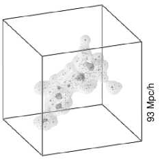
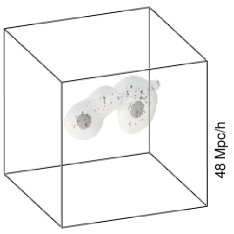
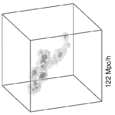
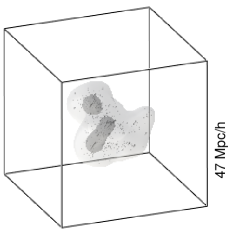
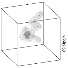
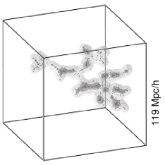
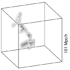
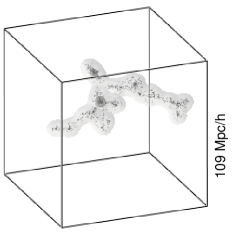
Figure 1: The density field view of the superclusters. We show with darker colours the central (core) region which approximately corresponds to the region for which the Minkowski functional $V_{3}$ has a maximum. Galaxies are shown with small dots. Upper panels from left to right: SCL126, SCL88, SCL9, SCL10. Lower panels from left to right: M1, M2, M3, M4.

The most prominent Abell supercluster in the Northern 2dF survey is the supercluster SCL126 (in E01, N152 in Paper I) in the direction of the Virgo constellation. This supercluster has been also called the Sloan Great Wall (Vogeley et al. vogeley04 (2004), Gott et al. gott05 (2005), Nichol et al. nichol06 (2006)).

Another rich supercluster in the Northern Sky is the Sextans supercluster, SCL88 (in E01; N20 in paper I). Only a small part of this supercluster is located inside the 2dF survey volume, including one of seven Abell clusters from this supercluster.

The richest supercluster in the Southern Sky is the Sculptor supercluster (SCL9 in E01; S34). This supercluster contains also several X-ray clusters. This supercluster contains the largest number of Abell clusters in our supercluster sample, 25. However, only 12 of then are located in the region covered by the 2dF redshift survey.

Another nearby prominent supercluster in the Southern sky is the Pisces-Cetus supercluster (SCL10 in E01, S5 in paper I) which contains the rich X-ray cluster, Abell 2734. Only one of 19 Abell clusters from this supercluster is located inside the 2dF survey boundaries. This supercluster was recently described as a rich filament of Abell clusters by Porter and Raychaudhury (pr05 (2005)).

From the Millennium simulation, we use the data on three richest superclusters. The supercluster M3 is 9th richest in the catalogue by the number of galaxies, but the reason to include this system in our analysis is that this supercluster is the second richest by the number of density-field (DF) clusters in it. Density-field clusters (Paper II) are local maxima of the luminosity density, and a counterpart to real galaxy clusters.

For comparison, we shall use the data on the best-known nearby supercluster, the Local Supercluster, denoted as V20 due to the chosen distance limit. The Local Supercluster represents a typical poor supercluster of a rather small size, with one rich galaxy cluster, the Virgo cluster, in the centre, surrounded by filaments of galaxies and poor groups. The Local Group is located near the edge of the supercluster. The total luminosity of the Local Supercluster is $L=3\times 10^{12}h^{-2}L_{\sun}$, and its mass is $M=1\times 10^{15}h^{-1}M_{\sun}$. Most superclusters in our catalogue of the 2dFGRS superclusters are of the Local Supercluster type (Paper I). The data on the Local Supercluster galaxies are taken from ZCAT (http://cfa- www.harvard.edu/$\sim$huchra/zcat/). In total we have in this supercluster 328 galaxies in a volume-limited sample ($M\leq-18.0$), with the maximum distance of 20 $h^{-1}$ Mpc.

The distribution of galaxies in regions of different density in real and simulated superclusters is shown in Fig. 1. We see at a first glance already how filamentary all the superclusters are. The presence of several concentration centres, as well as many high-density knots is also clearly seen.

3 Morphology of superclusters

3.1 Morphological descriptors

We characterize superclusters by their outer (isodensity) surface, and its enclosed volume. When increasing the isodensity level over the threshold overdensity $\delta=4.6$ (sect. 2.1), we move into the central parts of the supercluster. The morphology and topology of the isodensity contours is (in the sense of global geometry) completely characterized by four Minkowski functionals.

For a given surface the four Minkowski functionals are, respectively:

1. the first Minkowski functional $V_{0}$ is the enclosed volume V,

2. the second Minkowski functional $V_{1}$ is proportional to the area of the surface $S$, namely,

   $$V_{1}={1\over 6}S;$$ (1)

3. the third Minkowski functional $V_{2}$ is proportional to the integrated mean curvature C,

   $$V_{2}=\frac{1}{3\pi}C,\quad C=\frac{1}{2}\int_{S}\left(\frac{1}{R_{1}}+\frac{1}{R_{2}}\right)\,dS,$$ (2)

   where $R_{1}$ and $R_{2}$ are the two local principal radii of curvature.

4. the fourth Minkowski functional $V_{3}$ is proportional to the integrated Gaussian curvature (or Euler characteristic) $\chi$,

   $$V_{3}=\frac{1}{2}\chi,\quad\chi=\frac{1}{2\pi}\int_{S}\left(\frac{1}{R_{1}R_{2}}\right)dS.$$ (3)

The Euler characteristic is simply related to the genus, $G$

$$G = 1-V_{3}.$$ (4)

The fourth Minkowski functional gives us the number of isolated clumps (or voids) in the sample (Martinez et al. 2005; Saar et al. saar06 (2007)). One should beware of extra factors of 2 that are sometimes seen in formulae like (4); this error has crept into these two papers, too. With conventional normalization there should be no extra factors in (4).

To characterize the shape of an object Sahni et al. (sah98 (1998)) and Shandarin et al. (sss04 (2004)) introduced shapefinders, a set of combinations of Minkowski functionals: $H_{1}=3V/S$ (thickness), $H_{2}=S/C$ (breadth), and $H_{3}=C/4\pi$ (length). These quantities have dimensions of length and are normalized to give $H_{i}=R$ for a sphere of radius $R$. For a convex surface, the shapefinders $H_{i}$ follow the inequalities $H_{1}\leq H_{2}\leq H_{3}$. Prolate ellipsoids (pancakes) are characterized by $H_{1}<<H_{2}\approx H_{3}$, while oblate ellipsoids (filaments) are described by $H_{1}\approx H_{2}<<H_{3}$.

Additionally, Sahni et al. (sah98 (1998)) defined two dimensionless shapefinders $K_{1}$ (planarity) and $K_{2}$ (filamentarity): $K_{1}=(H_{2}-H_{1})/(H_{2}+H_{1})$ and $K_{2}=(H_{3}-H_{2})/(H_{3}+H_{2})$.

Then, after Sahni et al. (sah98 (1998)), the following shapes can be distinguished:

1. spheres with $H_{1}=H_{2}=H_{3}$, i.e. $K_{1}=K_{2}=0$;

2. ideal filaments with $K_{1}\approx 0$, $K_{2}\approx 1$;

3. real filaments with $K_{1}<K_{2}$;

4. ideal pancakes with $K_{1}\approx 1$, $K_{2}\approx 0$;

5. pancakes with $K_{1}>K_{2}$;

6. ideal ribbons with $K_{1}\approx K_{2}\approx 1$;

7. ribbons with $K_{1}/K_{2}\approx 1$.

In the $(K_{1},K_{2})$-plane filaments are located near the $K_{2}$-axis, pancakes near the $K_{1}$-axis, and ribbons along the diagonal, connecting the spheres at the origin with the ideal ribbon at $(1,1)$.

3.2 Supercluster morphology

Figure 2: The Minkowski functional $V_{3}$ (the Euler characteristic) (left panels) and the shapefinders $K_{1}$ (planarity) and $K_{2}$ (filamentarity) (right panels) for the observed (upper panels) and simulated (lower panels) superclusters. In the right panels we indicate for SCL126 and M1 with triangles the values of $K_{1},\leavevmode\nobreak\ K_{2}$, where the mass fraction $m_{f}=0.0$ (the whole supercluster), and for all superclusters with filled circles the values of $K_{1},\leavevmode\nobreak\ K_{2}$, which correspond to the $m_{f}$, at which $V_{3}$ has a maximum.

Figure 3: Shapefinders $H_{1}$ (thickness), $H_{2}$ (breadth), $H_{3}$ (length) (in $h^{-1}$ Mpc) for the observed superclusters (upper panels) and for the simulated superclusters (lower panels) versus the mass fraction $m_{f}$.

Figure 4: Shapefinders $K_{1}$ (planarity) and $K_{2}$ (filamentarity) for the observed superclusters (upper panels) and for the simulated superclusters (lower panels) versus the mass fraction $m_{f}$.

We present the results of our calculations of Minkowski functionals and shapefinders in Table LABEL:tab:2 and in Figures 2, 3 and 4. The original luminosity density field, used to delineate superclusters (Papers I, II), was calculated using all galaxies. For morphological study we have to use volume-limited galaxy samples; this makes our results insensitive to selection corrections. For this reason the density field had to be recalculated. We used for that a kernel estimator with a $B_{3}$ box spline as the smoothing kernel, with the total extent of 16 $h^{-1}$ Mpc (for a detailed description see Appendix and Saar et al. saar06 (2007)). This kernel covers exactly the 16 $h^{-1}$ Mpc extent of the Epanechnikov kernel, used to obtain the original density field, but is smoother and resolves better density field details (its effective width is about 8 $h^{-1}$ Mpc). As the argument labeling the isodensity surfaces, we chose the mass fraction $m_{f}$ – the ratio of the mass in regions with density lower than the density at the surface, to the total mass of the supercluster. When this ratio runs from 0 to 1, the iso-surfaces move from the outer limiting boundary into the center of the supercluster, i.e. the fraction $m_{f}=0$ corresponds to the whole supercluster, and $m_{f}=1$ to its highest density peak.

In Table LABEL:tab:2 we give for all superclusters the values of the Minkowski functionals and shapefinders for two mass fraction values: $m_{f}=0.0$, which corresponds to the whole supercluster, and the value of $m_{f}$, at which the fourth Minkowski functional $V_{3}$ has a maximum (except for SCL126, see below) – this shows the maximum number of isolated cores (clumps) that the supercluster breaks into. At lower densities (mass fractions) these clumps are joined together, and at higher densities they start to disappear, when the density levels get higher than their maximum density.

Table 2: The Minkowski Functionals and shapefinders for rich superclusters.

ID	$m_{f}$	$V_{0}$	$V_{1}$	$V_{2}$	$V_{3}$	$H_{1}$ (T)	$H_{2}$ (B)	$H_{3}$ (L)	$K_{1}$(P)	$K_{2}$(F)	$K_{1}$/$K_{2}$
SCL126	0.0	1.27e5	2566.0	56.9	1	24.67	28.71	42.67	0.08	0.20	0.39
	0.89	1462	210.2	41.2	9	3.48	3.25	30.91	-0.03	0.81	-0.04
SCL88	0.0	2.84e4	743.10	24.44	1	19.11	19.36	18.33	0.01	-0.03	-2.36e-01
	0.65	927	103.40	15.33	3	4.48	4.29	11.50	-0.02	0.46	-4.71e-02
SCL9	0.0	1.75e5	3591.0	78.11	1	24.42	29.27	58.58	0.09	0.33	0.27
	0.79	3855	445.3	71.11	15	4.33	3.99	53.33	-0.04	0.86	-0.05
SCL10	0.0	3.72e4	885.80	27.11	1	20.97	20.80	20.33	-0.004	-0.01	0.35
	0.86	425	59.56	11.33	3	3.57	3.35	8.50	-0.03	0.43	-0.07
V20	0.0	3.05e4	736.90	23.33	1	20.72	20.11	17.50	-0.02	-0.07	0.22
	0.43	1589	121.60	11.56	2	6.53	6.70	8.67	0.01	0.13	0.10
M1	0.0	7.29e4	1649.00	42.56	1	22.09	24.67	31.92	0.06	0.13	0.43
	0.59	2354	244.00	33.89	5	4.82	4.58	25.42	-0.03	0.69	-0.04
M2	0.0	1.82e5	3772.0	77.78	1	24.18	30.87	58.34	0.12	0.31	0.40
	0.65	5930	644.0	91.89	15	4.60	4.46	68.92	-0.02	0.88	-0.018
M3	0.0	1.19e5	2624.0	63.67	1	22.64	26.24	47.75	0.07	0.29	0.25
	0.65	3860	420.9	60.00	9	4.59	4.47	45.00	-0.01	0.82	-0.02
M4	0.0	1.06e5	2381.00	58.00	1	22.26	26.13	43.50	0.08	0.25	0.32
	0.60	3454	374.90	55.78	9	4.61	4.28	41.84	-0.04	0.81	-0.05

The columns in the Table are as follows: column 1: Supercluster ID, column 2: mass fraction, $m_{f}$, columns 3–6: Minkowski functionals $V_{0}$ – $V_{3}$, $V_{0}$ in ($h^{-1}$ Mpc)³, $V_{1}$ in ($h^{-1}$ Mpc)², $V_{2}$ in $h^{-1}$ Mpc, columns 7–9: shapefinders $H_{1}$ (thickness), $H_{2}$ (breadth) and $H_{3}$ (length), in $h^{-1}$ Mpc, columns 10–12: shapefinders $K_{1}$ (planarity), $K_{2}$ (filamentarity) and their ratio, $K_{1}/K_{2}$.

At small mass fractions the iso-density surface includes the whole supercluster. Thus volumes and areas of superclusters ($V_{0}$ and $V_{1}$, Table LABEL:tab:2) are large. As we move to higher mass fractions, the iso-density surfaces include only higher density parts of superclusters, and their volumes and areas get smaller. At very high mass fractions only the highest density clumps in superclusters give their contribution to the supercluster. Individual high density regions in a supercluster, which at low mass fraction are joined together into one system, began to separate from each other, and the value of the fourth Minkowski functional ($V_{3}$) increases. At a certain density contrast (mass fraction) $V_{3}$ has a maximum showing the largest number of isolated clumps in a given supercluster at the spatial resolution determined by the smoothing kernel. At still higher density contrasts only the highest density peaks contribute to the supercluster.

Figure 2 (left panels) shows the fourth Minkowski functional $V_{3}$ for the most massive real and simulated superclusters. The $V_{3}$ curve for the supercluster SCL9 in the left upper panel shows a characteristic behaviour. At the mass fraction value of about 0.2, the value of $V_{3}$ for SCL9 begins to increase and reaches a maximum value at the mass fraction $m_{f}\approx 0.7$. Then the values of $V_{3}$ begin to decrease. This indicates that the overall morphology of the supercluster SCL9 is clumpy; this supercluster consists of a large number of clumps or cores connected by relatively thin filaments, in which the density of galaxies is too low to contribute to the supercluster, starting at certain mass fraction values. The maximum value of the fourth Minkowski functional $V_{3}$ shows that the supercluster SCL9 has the largest number of isolated clumps in it, although this supercluster is only partly covered by our sample – the value of $V_{3}$ for the whole supercluster may be twice as large as our present calculations show. This supercluster is the largest and richest of observed superclusters in our present sample, with the largest size and volume.

The second richest and largest supercluster among the observed superclusters is the supercluster SCL126. Figure 2 shows that the $V_{3}$ curve for SCL126 has a shape which is quite different from that for SCL9. At a mass fraction $m_{f}\approx 0.4$ the values of $V_{3}$ increase rapidly, has a peak, decreases again and has another peak at a mass fraction of about $m_{f}\approx 0.85$. This behaviour of the $V_{3}$ curve indicates that the overall morphology of the supercluster SCL126 is rather homogeneous, which is characteristic to a rich filament with several branches (see also Sect. 3.3). Interestingly, the $V_{3}$ curve for the supercluster SCL126 shows several peaks at a high mass fraction, $m_{f}>0.95$. This indicates the presence of a very high density core region with several individual clumps in it – this is the main core region of the supercluster with several Abell clusters, which are also X-ray clusters (Einasto et al. 2003d ). In other superclusters we do not see such a high density and very compact core. An example of a supercluster with a high density core is the simulated supercluster M2, but in this supercluster the peaks at high mass fraction in the $V_{3}$ curve appear at mass fractions $m_{f}<0.95$.

In Figure 2 the observed superclusters separate clearly into two different classes. The superclusters SCL88 and SCL10 have much smaller numbers of density peaks than the superclusters SCL126 and SCL9. This may be partly explained by the incompleteness of the SCL10 and SCL88, which are cut by the survey boundaries. In the case of the Virgo supercluster V20 the maximum value of the fourth Minkowski functional is only 2, describing a compact supercluster.

The shapes of the $V_{3}$ curves for simulated superclusters in Figure 2 and their maximum values show large variations. In the case of the supercluster M2 the $V_{3}$ curve shows a rapid increase at the mass fraction $m_{f}\approx 0.4$, and three maxima, one of them at $m_{f}\approx 0.9$. This shows that this supercluster is very clumpy. The maximum value of $V_{3}$ is comparable to that for the observed supercluster SCL9, and the presence of a peak at high values of $m_{f}$ is comparable to that for SCL126. However, the mass fraction at which the peak occurs is lower than in the case of SCL126.

The shapes of the $V_{3}$ curves for simulated superclusters M3 and M4 resemble those for the observed supercluster SCL9; however, the maximum values of $V_{3}$ are less than 10, showing that the number of isolated cores or clumps in these simulated superclusters is smaller than in SCL9. The simulated supercluster M1 has the smallest maximum value of $V_{3}$ among simulated superclusters showing that this supercluster is less clumpy than other simulated superclusters. The number is isolated clumps in this supercluster is still larger than that for the observed superclusters SCL10 and SCL88.

We have determined the number of density field clusters in superclusters (Paper I). Tables LABEL:tab:1 and  LABEL:tab:2 show that in all superclusters except SCL88 and M4 the maximum value of $V_{3}$ is about half the number of density field clusters indicating that typically high density cores in superclusters contain two density field clusters. In superclusters SCL88 and M4 these values are equal.

The value of $V_{3}$ for SCL9 and M2 is negative at the mass fraction $m_{f}\approx 0$, indicating that there are holes through the supercluster.

Next we analyze the shapefinders $H_{1}$-$H_{3}$ for superclusters. These quantities have dimensions of length, and $H_{1}\leq H_{2}\leq H_{3}$ in the case of a convex body (e.g., triaxial ellipsoid). Therefore, they can be used to study the dimensions of superclusters. The shapefinder $H_{1}$ is the smallest and characterizes the thickness of superclusters. The shapefinder $H_{2}$ as an intermediate one is an analogy of the breadth of a supercluster. The breadth is calculated as $H_{2}=S/C$, it contains information about both the area and curvature of an isodensity surface. The shapefinder $H_{3}$ is the longest and describes the length of the superclusters. Of course, this is not the real length of the supercluster, but a measure of the integrated curvature of the surface which may become very large for irregularly shaped and curved surfaces.

In Figure 3 (upper panels) we plot the shapefinders $H_{1}$ to $H_{3}$ for the richest superclusters. This figure shows that the extension of the superclusters as measured by the shapefinders $H_{1}$ and $H_{2}$ is about 15 – 20 $h^{-1}$ Mpc for the complete supercluster ($m_{f}=0$). At higher mass fractions, $m_{f}\approx 0.5$, the iso-surfaces include only higher density parts of superclusters, $H_{1}$ and $H_{2}$ are less than 10 $h^{-1}$ Mpc, i.e. the supercluster centers are still typical 3-dimensional objects. At those mass fractions which correspond to the maximum value of $V_{3}$ (the core regions of superclusters) $H_{1}$ and $H_{2}$ are of about 5 $h^{-1}$ Mpc. The scatter of the shapefinder $H_{2}$ for observed superclusters is larger than that of $H_{1}$ showing the influence of a different number of substructures (isolated clumps or cores) in these systems.

The shapefinder $H_{3}$ differs strongly for the four observed superclusters. For the whole superclusters ($m_{f}=0$) the values of $H_{3}$ are about 20$h^{-1}$ Mpc for poorer superclusters and 40 – 60 $h^{-1}$ Mpc for the two richest superclusters, SCL126 and SCL9. We note that for the richest two superclusters at mean mass fractions $m_{f}\approx 0.5$ the value of $H_{3}$ is larger than at $m_{f}=0$, reaching a maximum value of about 60 – 80 $h^{-1}$ Mpc. This shows their complicated structure with subsystems of large curvature. The value of $H_{3}$ is the largest in the case of the supercluster SCL9, which is the longest supercluster with the largest number of isolated clumps or cores in it. In the case of other observed superclusters the value of $H_{3}$ decreases when we increase the mass fraction and move into the central parts of the superclusters. This is additional evidence that these superclusters are less clumpy than SCL9 and SCL126. At mass fractions $m_{f}\approx 0.5$ the value of $H_{3}$ for these superclusters is less than 20 $h^{-1}$ Mpc.

Figure 3 (lower panels) shows the shapefinders $H_{1}$-$H_{3}$ for simulated superclusters. We see that the shapefinder $H_{1}$ (thickness) for the simulated superclusters has values close to those for observed superclusters, but with a much smaller scatter. The breadths of the simulated superclusters ($H_{2}$) have values intermediate between those for the observed superclusters SCL9 and SCL126, and for other observed superclusters. Again, the scatter of these values is very small. Therefore, the shapefinders $H_{1}$ and $H_{2}$ for the model superclusters show an astonishing universality.

The shapefinder $H_{3}$ (length) shows a rather different picture. The curve for the simulated supercluster M2 is rather similar to that for the observed supercluster SCL9; $H_{3}$ for the superclusters M3 and M4 are close to that for SCL126. The length of the shortest simulated supercluster M1 is still larger than the length of the shortest observed superclusters, SCL10, SCL88, and the Local supercluster. The large values of $H_{3}$ at intermediate mass fractions, $m_{f}\approx 0.5$ (30 and 90 $h^{-1}$ Mpc) indicate the presence of substructures in superclusters with high values of the curvature $C$.

Next we study the shapefinders $K_{1}$ and $K_{2}$ for the richest superclusters (Figure 4). $K_{1}$ is defined by the thickness $H_{1}$ and the breadth $H_{2}$, this characterizes the planarity of the superclusters; $K_{2}$ is calculated from the breadth $H_{2}$ and the length $H_{3}$ and this parameter characterizes the filamentarity of superclusters.

In the upper panels of Fig. 4 we present the planarity and the filamentarity for observed superclusters. The values of the planarity $K_{1}$ for the full superclusters (the mass fraction $m_{f}=0$) are 0.10–0.15 for the richest superclusters, SCL126 and SCL9, and about 0.05 for other observed superclusters. As the mass fraction increases and only the higher density parts contribute to superclusters, the values of the planarity $K_{1}$ start to decrease. For the supercluster SCL126 the $K_{1}$ curve has a small minimum at the mass fraction $m_{f}\approx 0.4$; this is the mass fraction value at which the value of the fourth Minkowski functional $V_{3}$ starts to increase. In superclusters the value of $K_{1}$ for the core regions becomes negative. This shows that at very high mass fractions, which include only the central regions of superclusters, the isodensity surfaces have complex shapes, different from the heuristic classification based on convex ellipsoids as described above.

The values of the filamentarity for observed superclusters, $K_{2}$, have much larger scatter than the values of the planarity, $K_{1}$. For the richest superclusters, SCL126 and SCL9, $K_{2}\approx 0.2-0.3$, the other observed superclusters have smaller $K_{2}$ (at the mass fraction $m_{f}=0$). The central parts of these superclusters (at high values of mass fractions) are more filamentarity than the full superclusters. The Virgo supercluster V20 has a different shape, for this supercluster the the filamentarity $K2$ decreases for $mf<0.2$.

In the case of simulated superclusters, the filamentarities $K_{2}$ have a smaller scatter than those for the observed superclusters. The simulated supercluster M2 has the largest value of $K_{2}$ in our sample, $K_{2}\approx 0.6$, other simulated superclusters have $K_{2}\approx 0.3-0.5$, similar to the observed superclusters SCL126 and SCL9 (for the whole supercluster).

In earlier studies the shapes of superclusters have been characterized using the ratio $K_{1}$/$K_{2}$ for the full superclusters (Basilakos et al. bpr01 (2001); Basilakos bas03 (2003)). We plot this ratio for the whole mass fraction interval in Figure 4, right panels. This Figure shows that the ratios $K_{1}$/$K_{2}$ for the observed and simulated superclusters are rather similar, having values of about 0.25–0.4. This shows a high degree of filamentarity in the case of the whole superclusters. The ratios $K_{1}$/$K_{2}$ slowly decrease, as we increase the mass fraction and move to central regions of superclusters. Exceptions are the observed supercluster SCL10 with the highest values of $K_{1}$/$K_{2}$ at intermediate mass fractions, and the Virgo supercluster V20 for which this ratio changes strongly.

The information about the shapes of superclusters can be best described by their morphological signature, the path in the shapefinder $K_{1}$-$K_{2}$ plane for varying $m_{f}$ (Figure 2, right panels), both for the observed and model superclusters. To show which part of the shape plane corresponds to the whole supercluster, we mark with triangles the values of $K_{1},K_{2}$ at the mass fraction $m_{f}=0$ for the superclusters SCL126 and M1. We also mark with circles the values of $K_{1},K_{2}$ at the mass fraction corresponding to the maximum value of the fourth Minkowski functional $V_{3}$ (Table LABEL:tab:2). As explained in Appendix B, we restrict the $m_{f}$ from below, starting the curves from $m_{f}=0.01$. This is done to eliminate the influence of the slight non-isotropy of the $B_{3}$ kernel at low densities.

In the shapefinder plane $K_{1}$-$K_{2}$, the observed superclusters SCL126 and SCL9, and the simulated superclusters have similar trajectories. As we change the mass fraction, the $K_{1}$–$K_{2}$ shapefinder path moves from low $K_{1}$ and $K_{2}$ values (this corresponds to the whole supercluster and low mass fractions) to the upper left region with higher $K_{2}$ and smaller $K_{1}$ (high mass fractions, the core of the supercluster). At first, as the mass fraction increases, the value of the shapefinder $K_{1}$ (the indicator of planarity) almost does not change, but the value of the shapefinder $K_{2}$ (the indicator of filamentarity) increases, in accordance to what we saw in Figure 4. At a certain mass fraction the value of the shapefinder $K_{2}$ reaches it’s maximum value. As we still increase the value of the mass fraction (and move to higher densities, into the cores of superclusters), the value of the shapefinder $K_{2}$ changes a little, but the value of the shapefinder $K_{1}$ decreases.

We see that the richest superclusters have a distinct signature in the shapefinder $K_{1}$-$K_{2}$ plane – a characteristic curve which describes the typical morphology of superclusters. This signature is characterized by an rising path with a small fixed positive $K_{1}$, a plateau at the maximum value of $K_{2}$, and a descending branch at a small fixed negative value of $K_{1}$. In Appendix we shall show that this curve is characteristic to multi-branching filaments.

The large scatter of the different curves in the $K_{1}$–$K_{2}$ plane is remarkable. Among the observed superclusters, we find two types of behaviour. The scatter of the trajectories for the model superclusters is smaller.

So, in summary, superclusters are extended 3-dimensional objects composed of multi-branched filaments. The clumpiness of superclusters can be quantified by the fourth Minkowski functional $V_{3}$ which determines the number of isolated cores or clumps in superclusters. The shape of the $V_{3}$ curve gives us information about the overall morphology of the superclusters (a rich filament with several branches in the case of SCL126, clumpy in the case of other superclusters). In the $K_{1}$–$K_{2}$ shapefinder plane the morphology of superclusters is described by a curve (morphological signature), which is characteristic to multi-branching filaments. In case of the Virgo supercluster we see how the Minkowski functionals and shapefinders describe a compact supercluster with one central cluster and accompanying filaments, where poorer clusters and groups of galaxies reside. The morphological signature for the Virgo supercluster is characteristic to a spider – a supercluster with one central body, surrounded by filaments (see Appendix).

Using the data in Table LABEL:tab:2 we can estimate that in high density regions of superclusters (at mass fractions where the value of the fourth Minkowski functional has a maximum) the density of galaxies is of about ten times higher than the mean density of galaxies in the same supercluster.

Figure 5: The fourth Minkowski functional $V_{3}$ for the bright (B, $M\leq-20.0$) and faint (F, $M>-20.0$) galaxies of the observed superclusters (upper panels, from left to right: SCL126, SCL88, SCL9 and SCL10) and for the Millennium simulation (lower panels, from left to right: M1, M2, M3, M4).

3.3 Distribution of bright and faint galaxies

As a further application of Minkowski functionals we investigate the distribution of bright and faint galaxies in rich superclusters. We divide galaxies into populations of bright and faint galaxies using a bright/faint galaxy limit $M_{bj}=-20.0$. The same division was used in Paper III (Einasto et al. 2007c) to study the distribution of bright and faint galaxies in superclusters. Next we calculate the Minkowski functionals separately for these two populations of galaxies, for both real and simulated superclusters.

The fourth Minkowski functional, $V_{3}$, for the bright and faint galaxies in the observed and simulated superclusters is shown in Fig. 5. We see that there are large differences of the fourth Minkowski functional for these populations in observed superclusters. This Minkowski functional characterises the clumpiness of superclusters. In the supercluster SCL126 a high level of clumpiness is observed over a large range of mass fractions, both for the bright and faint galaxies. For the bright galaxies $V_{3}$ reaches a value of about 10, while for the faint galaxies the value of $V_{3}$ remains about 5. In the supercluster SCL9 the clumpiness of both the bright and faint galaxies is peaked at a rather high value of the mass fraction, but for the bright galaxies in a broader mass fraction range. In the superclusters SCL88 and SCL10 the clumpiness is very low, again for galaxies of both brightness classes. The fact that the values of $V_{3}$ for the bright galaxies are larger than for the faint galaxies shows that the bright galaxies are located in numerous clumps or cores while the fainter galaxies form a less clumpy population around them.

In contrast, the values of $V_{3}$ for the bright and faint galaxies in simulated superclusters differ less than in the case of the observed superclusters. Therefore, the clumpiness of the bright and faint galaxies in model superclusters is rather similar. The reason for this difference between the real and model superclusters is not yet clear; one possible explanation is that the luminosity-density correlation is not modeled well. In Paper I we showed that, on large scales, the luminosity–density relation is built into the Millennium Simulation galaxy sample. However, at small scales there are large differences of clumpiness between these samples; this represents the largest difference between the real and simulated galaxy populations found in this paper.

4 Discussion

4.1 Shapes and sizes of superclusters

To characterize the shape of an object Sahni et al. (sah98 (1998)), Sheth et al. (sheth03 (2003)) and Shandarin et al. (sss04 (2004)) have investigated the morphology of simulated superclusters and voids using the Minkowski functionals and shapefinders. They studied, among others, the largest (percolating) supercluster, and showed that according to shapefinders, this system is filamentary. Sheth et al. (sheth03 (2003)) plotted the morphology of the largest (percolating) supercluster in the shapefinder $K_{1}$-$K_{2}$ plane for a limited interval of threshold densities. In this paper the shapefinder $H_{3}$ was defined differently from their earlier definition. However, if we recalculate our shapefinder in the same way as Sheth et al. (sheth03 (2003)), we get rather similar shape curves as their Fig. 18.

The shapes and sizes of the observed superclusters were studied by Basilakos et al. (bpr01 (2001)), Kolokotronis et al. (kbp02 (2002)), and by Basilakos (bas03 (2003)), and those of LCDM superclusters by Basilakos et al. (bas06 (2006)) using Minkowski functionals and shapefinders for the density field, that was smoothed with a Gaussian kernel. Kolokotronis et al. (kbp02 (2002)) calculated the shapefinders $K_{1}$, $K_{2}$, and their ratio $K_{1}/K_{2}$ for Abell superclusters and showed that about 50% of all superclusters have the ratio $K_{1}/K_{2}<1$ as is typical for filaments. They also showed that the ratio $K_{1}/K_{2}$ is larger for poor superclusters, which are typically planar structures (pancakes), and smaller for rich superclusters, which are more filamentary. This agrees also with our study which showed that the richest superclusters are multi-branching filaments. Similarly, Basilakos (bas03 (2003)) showed that at least 70% of superclusters from their SDSS supercluster catalogue are of filamentary type (the shapefinder $K_{1}/K_{2}<1$). They showed that also in models filamentary superclusters dominate.

We expand this approach by using the Minkowski functionals and shapefinders to analyze the full density distribution in superclusters, at all density levels.

In paper II we presented a detailed comparison of sizes and shapes of superclusters using a number of parameters. First of all, we calculated the maximum and effective diameters of superclusters (the maximum diameter is the maximum distance between the grid vertices belonging to the supercluster, and the effective diameter is the diameter of a sphere with a volume equal to that of the supercluster). In order to characterize the compactness of the supercluster, we used the ratio of these two diameters, the maximum to the effective. This ratio is the larger, the more empty space is located in the sphere circumscribed around the supercluster (the more filamentary the supercluster is). We showed that superclusters are mainly filamentary objects. Also we calculated the distance between the dynamic centers of the superclusters (defined by the position of the highest density cluster), and the geometric center (defined by the mean of the maximum coordinate values along the $x,\leavevmode\nobreak\ y,\leavevmode\nobreak\ z-$axes); this parameter characterizes the asymmetry of superclusters. Our study showed that rich superclusters are more filamentary, less compact and more asymmetrical than poor superclusters.

The Local Supercluster as the closest and best studied supercluster serves as a supercluster template for poor superclusters, which are the most numerous superclusters in our catalogue. As seen in the morphology figures, its morphology is still different from that of other superclusters in the present selection (see, especially, the $K_{1}/K_{2}$ ratio and its morphological signature in the $K_{1}$-$K_{2}$ plane).

4.2 The peculiar supercluster SCL126

One of the two richest superclusters from the 2dF survey catalogue is the supercluster SCL126 in the Northern sky. In the $K_{1}$-$K_{2}$ shapefinder plane this supercluster is modeled as a multi-branching filament. The $V_{3}$ curve for SCL126 has peaks at very high mass fractions ($m_{f}>0.95$) – an indication of a high density compact core. In Einasto et al. (2003d ) we showed that the core region of this supercluster contains several Abell clusters, which are also X-ray clusters. This region has a size of about 10 $h^{-1}$ Mpc. This supercluster is located almost perpendicularly to the line-of-sight (Jaaniste et al. ja98 (1998), Einasto et al. 2003d ). In paper RII we shall show that the fraction of star-forming galaxies, especially in the core region, in this supercluster is lower than in the supercluster SCL9. A possible interpretation of these findings is that this supercluster started to form earlier than the supercluster SCL9.

The Minkowski functionals and shapefinders indicate that this supercluster resembles a rich filament with several branches, and is less clumpy than other richest superclusters (SCL9, and simulated superclusters). This interpretation agrees with the description of this supercluster as a wall in other papers (the Sloan Great Wall, Vogeley et al. vogeley04 (2004), Gott et al. gott05 (2005) and gott06 (2006), Nichol et al. nichol06 (2006)). This supercluster affects the measurements of the correlation function (Croton et al. croton04 (2004)), and the genus and Minkowski functionals of the SDSS and 2dF redshift surveys (Park et al. park05 (2005); Saar et al. saar06 (2007)). The ”meatball” shift in the measurements of the topology in the SDSS data is partly due to this supercluster (Gott et al. gott06 (2006)). Gott et al. conclude that N-body simulations with very large volume and more power at large scales are needed to model such structures more accurately than present simulations. Similar conclusions were reached by Einasto et al. (e06c (2006)).

5 Conclusions

We used a catalogue of superclusters of galaxies for the 2dF Galaxy Redshift Survey and a catalogue of model superclusters from the Millennium Simulation to study the morphology and internal structure of the richest superclusters. Our main conclusions are the following.

• The morphology of superclusters can be quantified, using the Minkowski functionals and shapefinders.

• The fourth Minkowski functional $V_{3}$ describes well the clumpiness of superclusters. The value of $V_{3}$ indicates that the supercluster SCL126 resembles a multibranching filament, while the supercluster SCL9 can be described as a collection of spiders (a multispider), consisting of a large number of cores connected by relatively thin filaments. Simulated superclusters (especially M2) have $V_{3}$ curves that are somewhat different from those for observed superclusters.

• We show, using empirical geometrical models, that the trajectory traced by the supercluster when we change the mass fraction, forms a curve in the $K_{1}$-$K_{2}$ plane (the morphological signature), which is characteristic to multibranching filaments.

• The Minkowski functionals and shapefinders for observed superclusters have a much larger scatter than those for simulated superclusters. The Millennium superclusters show very similar morphological scaling relations ($H_{1}(m_{f}),H_{2}(m_{f}),K_{1}(m_{f}),K_{1}/K_{2}(m_{f})$), while these curves vary considerably for the observed superclusters.

• The values of the fourth Minkowski Functional $V_{3}$ show that the clumpiness of real superclusters, for galaxies of different luminosity, has a much larger scatter than the clumpiness of model superclusters. This may be an indication that the luminosity-density relation in the models does not reflect well the real situation.

The present analysis supplements the previous work, adding more details and using the Minkowski functionals in a novel way. In summary, different methods describe together many aspects of the morphology of superclusters – their sizes, shapes, volumes, compactness and clumpiness, giving an overall picture of their morphology.

Appendix A Morphological templates

While shapefinders have been used in a number of papers, their meaning needs clarification. In the original paper (Sahni et al. sah98 (1998)) they were illustrated by calculating them for regular geometric bodies (ellipsoids and tori). The superclusters we find from observations are more complex, frequently branching structures, and kernel estimators give us, as a rule, corrugated density isosurfaces. So, in order to understand better the shapefinders, we calculate them first for a well-known household object, a common kitchen table, and then for several possible supercluster templates.

We build the table by adding layers of different density to a skeleton, consisting of a plate of the size of $40\times 100$ (grid units), and of four legs (rods) of the length of $60$, which join the plate perpendicularly at its corners. We use the parabolic density law:

$$\varrho(r)=1-r^{2}/R^{2},\quad r\leq R;\varrho(r)=0,\quad\mathrm{otherwise},$$

where $r$ is the nearest distance from a point to the skeleton, and we have taken the limiting distance $R=10$ grid units. This is a rather thick table with thick legs; the reason for that is the following. First, as we use Crofton formulae to calculate the Minkowski functionals, we have to ensure that our table occupies a generic position in space (the specific weights we use are obtained by assuming statistical isotropy of the isodensity surfaces, see Schmalzing and Buchert (jens97 (1997))). We do this by aligning the normal to the plate in the direction ${\mathbf{n}}=(1/\sqrt{3},1/\sqrt{3},1/\sqrt{3})$. As the plate is inclined with the respect to the coordinate grid, the isosurfaces are inevitably slightly jagged, and large $R$ makes them smoother. When following the density isosurfaces inwards, towards larger $m_{f}$, we find another effect – because of the inclination of the skeleton the high density regions on the grid break up into a large number of isolated clumps around grid points. So we shall present the shapefinders only for mass fractions $m_{f}\leq 0.93$ (up to the break-up). The shapefinders are given in Fig. 6, for the full table, for the plate, for a single leg and for four legs together.

Figure 6: The shapefinders $H_{1}$ (thickness), $H_{2}$ (width), $H_{3}$ (length), upper row, and $K_{1}$ (planarity), $K_{2}$ (filamentarity), and the morphological signature for the table and its details.

Let us start with the first shapefinder, the thickness $H_{1}$. We know by construction that the true thickness is $2R=20$ at the outer edges of the table, and reaches 0 inside. The Figure shows that $H_{1}$ almost finds the true thickness for the plate, is slightly lower for the leg(s), starting from 13, and runs in between those two relations for the full table.

The second shapefinder, $H_{2}$, should give the width of the table. For the plate it should be $40+2R=60$ at low densities and 40 at high densities. As we see, it runs from about 33 to 22, more close to the half-width of the plate; this is logical, considering that the shapefinders are normalized requesting that the ’width’ of a sphere should equal its radius, not diameter. But a similar normalization is used for the thickness above, which, however, finds the full thickness. The width of the leg(s) is equal to their thickness, $H_{1}=H_{2}$ – the legs are cylinders. And the ’width’ (half-width, to be more precise) of the table, the combination of the above details, is closer to the widths of the legs; these four appendices dominate the width shapefinder for the full table.

The third shapefinder $H_{3}$ should give the length of the objects. It starts from about 47 for the plate, and from 28 for a leg. Here, finally, the shapefinder for four legs is four times that for a single leg, as it should be. But these values show that $H_{3}$ gives really the half-length of the object, because of the normalization, again. And the half-length of the full table is larger than any of its details, but does not equal their sum. Moreover, while the lengths of the details approach those of the skeleton, the length of the full table stays, surprisingly, the constant.

The ’second-order’ shapefinder, the planarity $K_{1}$, is small (about 0.06) for the leg(s), runs from 0.27 (thick plate) to 0.8 (fat skeleton) for the plate, and from 0.18 to 0.6 for the full table. These numbers are as expected, only the maximum planarity for the plate seems to be too small; but, as explained above, this might be simply a non-aligned grid effect.

The filamentarity $K_{2}$ is smallest for the plate, ranging from 0.17 to 0.27. It is not too large for a single leg (from 0.3 to 0.7, the legs are thick), but ranges from 0.76 to 0.92 for the collection of four legs. The filamentarity of the full table is dominated by that of the legs; it ranges from 0.64 to 0.85; a kitchen table is basically a filamentary object.

The planarity/filamentarity ratio $K_{1}/K_{2}$ that is frequently used, runs from 0.2 to about 0.1 for a single leg, and is lower than 0.07 for the collection of four legs. It is high (larger than 1.5) for the plate, but pretty low (between 0.5 and 0.7) for the full table; another indication that legs define the morphology of a table. This curve is pretty jaggy, and the reason for that is clear – the ’first order’ shapefinders $H_{i}$ are ratios of Minkowski functionals, the ’second order’ shapefinders $K_{i}$ are ratios of these ratios, and the ratio $K_{1}/K_{2}$ become extremely noisy.

We can also look at the morphological signatures (the trajectories in the $K_{1}$–$K_{2}$ plane, parameterized by $m_{f}$) of the table and its details (Fig. 6, lower right panel). We limit the mass fraction range for this figure also from below, using only $m_{f}\in[0.01,0.94]$, as done in the main paper (see also appendix B). This choice eliminates grid effects at low densities.

Ignoring the jaggy nature of the curves (these can be eliminated, in principle, by constructing direct estimates for the shapefinders $K_{1}$ and $K_{2}$) we see that the details and the table have clear and distinct signatures. The signature for the plate lies in the planar region, that for the leg(s) in the region describing filaments (and four legs together are clearly more filamentary than a single leg). The full table is both planar $K_{1}\in[0.2,0.7]$ and filamentary $K_{2}\in[0.65,0.9]$, but clearly rather filamentary than planar ($K_{2}>K_{1}$).

The kitchen table was an example of a smooth density distribution. The density of our superclusters is obtained by summing together almost isotropic kernels around galaxy locations. This results in a much more patchy density distribution; on the other hand, it automatically guarantees statistical isotropy of the density isolevels. In order to better understand the shapefinders of the observed superclusters, we calculate them for a number of simple templates that resemble the superclusters. These are: 1) a single long filament, 2) a spider (two long filaments, crossing, with a small cube at the centre), 3) Jacob’s staff or ballestina (an astronomical instrument from middle ages for measuring angular distances; a long staff with a perpendicular smaller staff), and 4) the Cross of Lorraine (similar to the Jacob’s staff, but with two perpendicular staves, with a spherical blob at the centre). The last configuration resembles also ancient petroglyphs from Karelia, depicting thunder and reindeer. The dimensions are: 100 (grid units) for the filament (and staff) length, 40 for the small staff length, 10 for the radius of the blob, and the effective width of the density kernel is 8 (total width 16). The corresponding shapefinders are shown in Fig. 7.

Figure 7: The shapefinders $H_{1}$ (thickness), $H_{2}$ (width), $H_{3}$ (length), upper row, and $K_{1}$ (planarity), $K_{2}$ (filamentarity), and the morphological signature (lower row) for different templates. The labels are: 1 – filament, 2 – spider, 3 – Jacob’s staff, and 4 – Cross of Lorraine (Karelian reindeer).

As we see, the shapefinders are smoother, and clearly distinct for different morphologies. The complex (corrugated) nature of the isodensity surfaces causes local minima for the lengths $H_{i}$ at certain mass fractions (in the thickness and in the width of the spider). Also, the length shapefinder $H_{3}$ almost does not change for a wide initial interval of mass fractions, while the isodensity surfaces contract towards the skeletons of our templates. As this length is defined both by the isodensity surface area and its curvature, a simple behaviour cannot be always expected.

A new feature here is that the ’second order’ shapefinder $K_{1}$ acquires negative values for specific density isolevels. This is possible, as the inequalities $H_{1}\leq H_{2}\leq H_{3}$ that are usually assumed, are valid only for convex bodies. The isolevels for kernel-estimated densities are usually corrugated, and the real limits for $K_{i}$ are: $K_{i}\in[-1,1]$. This may forbid the use of the usual morphological index $K_{1}/K_{2}$; it is better to use the ’morphological signature’ $K_{2}$ versus $K_{1}$ instead.

Looking at Fig. 7 we see that there are two morphologies that resemble those of the observed superclusters. The ’spider’ imitates poor Virgo-type superclusters, although our model spider has a large value $K_{2}$, rich superclusters (as SCL126, see Fig. 2) are best represented by the Cross of Lorraine, a multibranching filament. Adding a central body to that system improves the similarity yet more.

We do not attempt to fit supercluster models to observations in this paper; this will need a well-parameterized basic model. However, we see that a good starting point for such a project would be the two models listed above.

Appendix B Kernel densities

When studying the morphology of superclusters of galaxies, a necessary step is to convert the spatial positions of galaxies into spatial densities. The standard approach is to use kernel densities (see, e.g., Silverman silverman (1986)):

$$\varrho(\mathbf{x})=\sum_{i}K(\mathbf{x-x}_{i};h)m_{i},$$

where the sum is over all galaxies, $\mathbf{x}_{i}$ are the coordinates of the $i$-th galaxy, and $m_{i}$ is its mass (or luminosity, if we are estimating luminosity densities; for number densities we set $m_{i}\equiv 1$). The function $K(\mathbf{x};h)$ is the kernel of the width $h$, and a suitable choice of the kernel determines the quality of the density estimate. If the kernels widths depend either on the coordinate $\mathbf{x}$ or on the position of the $i$-th galaxy, the densities are adaptive. We are using constant width kernels in this paper, defining superclusters as density enhancements of a common scale (the typical density scale of about 8$h$ Mpc^-1). Kernels have to be normalized and symmetrical:

$$\int K(\mathbf{x};h)dV=1,\qquad\int\mathbf{x}K(\mathbf{x};h)dV=0.$$

Statisticians classify kernels by their MSE (minimal standard error); the best kernel is the Epanechnikov kernel $K_{E}$:

$$K_{E}(\mathbf{x};h)=\frac{15}{8\pi h^{3}}(1-\mathbf{x}^{2}/h^{2})\;,\quad\mathbf{x}^{2}\leq h^{2},\;\quad 0\quad\mathrm{otherwise}\;.$$

(all the kernel expressions in this appendix are for 3-D kernels).

In cosmology, the Gaussian kernel $K_{G}$ has been the most popular:

$$K_{G}(\mathbf{x};h)=\frac{1}{(2\pi)^{3/2}h^{3}}\exp\left(-\mathbf{x}^{2}/2h^{2}\right)\;.$$ (5)

For the usual case, when densities are calculated for a spatial grid, good kernels are generated by box splines $B_{J}$ (these are usually used in $N$-body mass assignment). Box splines have compact support (they are local), and they are interpolating on a grid:

$$\sum_{i}B_{J}(x-i)=1,$$

for any $x$, and a small number of indices that give non-zero values for $B_{J}(x)$. In this paper we restrict us to the popular $B_{3}$ splines:

$$B_{3}(x)=\frac{1}{12}\left[|x-2|^{3}-4|x-1|^{3}+6|x|^{3}-4|x+1|^{3}+|x+2|^{3}\right]$$

(this function is different from zero only in the interval $x\in[-2,2]$, see Fig 8). We define the (one-dimensional) $B_{3}$ box spline kernel of width $h=N$ as

$$K_{B}^{(1)}(x;N)=B_{3}(x/N)/N.$$

This kernel preserves the interpolation property (mass conservation) for all kernel widths that are integer multiples of the grid step, $h=N$. The 3-D $K_{B}^{(3)}$ box spline kernel we use is given by the direct product of three one-dimensional kernels:

$$K_{B}(\mathbf{x};N)\equiv K_{B}^{(3)}(\mathbf{x};N)=K_{B}^{(1)})(x;N)K_{B}^{(1)}(y;N)K_{B}^{(1)}(z;N),$$

where $\mathbf{x}\equiv\{x,y,z\}$.

Figure 8: Three popular kernels for density estimation – Epanechnikov, Gaussian, and the $B_{3}$ box spline. All the profiles have approximately the same extent (the Gaussian profile width $h=1$, the $B_{3}$ profile is given for $N=1$, and for the Epanechnikov profile $h=2$. All profiles are normalized for the 1-D case.

These kernels encompass all the good and bad kernel properties (good and bad for our application).

• First, the Epanechnikov and the $B_{3}$ kernels are both compact, while the Gaussian kernel is infinite and has to be cut off at a fixed radius. This introduces an extra parameter and, what is more important, generates small-amplitude density jumps that may distort the Minkowski functionals (these are extremely sensitive to small-amplitude density details).

• Second, the $B_{3}$ kernel conserves density (it is exactly normalized on a grid). For continuous kernels normalization on a grid is equivalent to simple numerical integration of the profile; the (truncated) Gaussian kernel demands less grid points for that than the Epanechnikov kernel. Many grid points inside the kernel profile means that kernel widths must be much larger than the grid step. Bad normalization leads to distortion of the final densities; how well the contribution of a galaxy to the final density is accounted for depends on the location of the galaxy with respect to the grid.

• Third, an important kernel property is its isotropy. The formulae that we use to estimate the Minkowski functionals assume average isotropy of the density isosurfaces (their isotropic orientation). Both the Epanechnikov and Gaussian kernels are exactly isotropic, the 3-D $B_{3}$ kernel is not. But this kernel is approximately isotropic to a high degree.

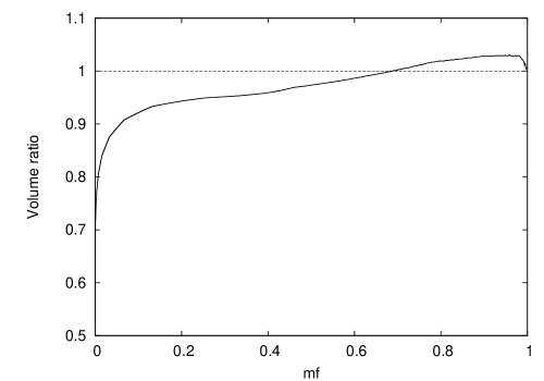
Figure 9: The ratio of the volume inside an isolevel to the volume of the sphere that cuts coordinate axes at the same point as the isolevel (an inscribed sphere for larger radii, an encompassing sphere for smaller radii). The isolevels are labeled by the ’mass fraction’, the kernel mass outside the isolevel. For an isotropic kernel this ratio should be 1.

A simple characteristic of isotropy of the kernel isolevels would be the ratio of its surface to the surface of the sphere that cuts coordinate axes at the same point as the isolevel. Alas, surfaces are not easy to calculate, and we replace this ratio by the ratio of the volumes encompassed by these two surfaces; volumes are easy to estimate by Monte-Carlo integration. These ratios are close (e.g., for a cube and the inscribed sphere the volume ratios coincide with the surface ratios). The dependence of this ratio (the sphere volume to the excursion set volume) as a function of the mass fraction (integrated kernel mass outside the isolevel) is shown in Fig. 9.

As we see, this ratio is close to unity for almost all mass fractions; considerable deviations can be seen only for small mass fractions. The deviation from isotropy is less than 10% for $m_{f}\geq 0.058$. When displaying our results on the morphological descriptors, we used a mass fraction limit for the full supercluster; this is smaller than the value cited above by the ratio of the number of galaxies defining the supercluster limits to the total number of galaxies in the supercluster. To be on a safe side, we knowingly underestimated this ratio and we chose the limit $m_{f}\geq 0.01$ for the full supercluster.