Cellular automata for traffic flow simulation with safety embedded notions

Abstract

In this paper a cellular automata model for one-lane traffic flow is presented. A new set of rules is proposed to better capture driver reactions to traffic that are intended to preserve safety on the highway. As a result, drivers behavior is derived from an analysis that determines the most appropriate action for a vehicle based on the distance from the vehicle ahead of it and the velocities of the two neighbor vehicles. The model preserves simplicity of CA rules and at the same time makes the results closer to real highway behavior. Simulation results exhibit the three states observed in real traffic flow: Free-flow states, synchronized states, and stop-and-go states.

,

1 Introduction

Traffic networks are very complex systems where elaborated topologies are combined with large number of vehicles running on the network. Predicting traffic behavior is very important for planning and operation purposes. In the last years, computer simulations as means for evaluating control and management strategies in traffic systems have gained considerable importance because of the possibility of taking into account the dynamical aspects of traffic.

In principle, traffic simulation models can roughly be divided into macroscopic and microscopic ones. While macroscopic models examine the dependencies between traffic flow, traffic volume, and average velocities; microscopic models investigate the movements of individual vehicles. In general, traffic flow models should keep the description of the relevant aspects of the flow dynamics as simply as possible by keeping track of the essential. In this spirit, Cellular Automata (CA) models for traffic flow were developed. Its main advantage is an efficient and fast performance when used in computer simulations, due to their rather low accuracy on a microscopic scale. These CA models for traffic flow are discrete in nature, in the sense that time advances with discrete steps, space is coarse-grained and properties of the CA can have only a finite, countable number of states allowing for high-speed simulations, especially when they are performed on a platform for parallel computation[1, 2, 3].

The basic idea of CA models is not to describe a complex system with complex equations, but let the complexity emerge by interaction of simple individuals following simple rules. Discrete space consists of a regular grid of cells, each one of which can be in one of a finite number $k$ of possible states. All cells are updated in a parallel way, in discrete time-steps. The new state of a cell is determined by the actual state of the cell itself and its neighbor cells. The discrete nature of CA makes it possible to simulate large traffic networks using a microscopic model faster than real time. In 1992 Nagel and Schreckenberg proposed a stochastic cellular automaton model of vehicular traffic [4], which was able to reproduce some empirically observed non-trivial traffic phenomena like spontaneous traffic jam formation². This publication captured the interest of the physicists community and ever since there has been a continuous progress in the development of cellular automata models of vehicular traffic. Recently, extended CA models for traffic flow have been proposed to reproduce even more subtle effects, like free flow, spontaneous jam formation, synchronized traffic and meta-stability. These models incorporate anticipation effects, reduced acceleration capabilities and an enhanced interaction horizon for braking [5, 6, 7]. Due to their design, cellular automata models are very efficient in large-scale network simulations [8, 9, 10, 11].

In this paper, a new CA probabilistic model for traffic simulation that incorporate modifications to the NaSch model trying to reach a compromise between fast simulations and fidelity of results is presented. The key idea is to preserve simplicity of CA rules and at the same time make them closer to real drivers behavior. Rules of vehicle interaction in [4] are modified to better capture driver reactions to traffic that are intended to preserve safety on the highway. As a result, vehicle behavior is based on a safety analysis that determines the most appropriate action for a vehicle to take, based on the distance from the vehicle ahead and its velocity. This analysis is inspired by the work presented in [12, 13, 14] for manual and automated highway systems. Although CA models can be applied to multiple lane highways, in this paper a one-lane highway with a ring topology is used. The goal is to show the ability of this CA model to capture the basic phenomena of traffic flow and preserve the simplicity and rapidity like the NaSch model.

Simulation results presented confirm that this CA model can reproduce most common regimes in traffic: free flow, synchronized flow and congested flow. The relations derived from the density/velocity and density/flow curves are in agreement with the empirical fundamental diagrams that describe these relations in traffic analysis. The influence of the variation of speed on the flow is also found to be a factor of great importance in traffic synchronization.

The paper is organized as follows. A description of the proposed CA model is presented in Section 2. In Section 3, simulation results in the form of fundamental diagrams and other useful traffic representations are analyzed. Special emphasis on the newly introduced safety based rules is given. Finally, Section 4 contains concluding remarks and a summary of findings.

2 Definition of the model

The model presented here is a probabilistic cellular automaton. It consists of $N$ vehicles moving in one direction on a one-dimensional lattice of $L$ cells arranged in a ring topology. The number of vehicles is fixed. Each cell can either be empty, or occupied with a single vehicle that spans one or more consecutive cells. The velocity of a vehicle is constrained to an integer in the range $\{0,\ldots,v_{max}\}$. In this paper, vehicles are allowed to occupy more than one cell. The speed limit, $v_{max}$ can be different depending on the kind of vehicle under consideration: trucks, cars, etc. For simplicity, in this paper only one type of vehicle is considered and therefore the same maximum velocity will be used for all vehicles. The integer velocity, that corresponds to one of the vehicle states in this CA, is related with the number of cells that a vehicle advances in one time step³. The other state, position, is related with the cell or cells that each vehicle is occupying.

Typical length of a cell, $\Delta x$, in [4] is $7.5\ m$, where it is interpreted as the length of a vehicle plus the distance between vehicles in a jam. In this paper, three lengths for each cell of the lattice are analyzed: $5.00$, $2.50$ and $1.25\ m$, with the idea of showing the influence of this length on simulation results⁴. The time step ($\Delta t$) is always taken to be $1\ s$, therefore, transitions are from $t\rightarrow t+1$. This time step is on the order of humans reaction time as pointed out in [15]. It can be easily modified. With these three values of $\Delta x$ and $\Delta t$, $v=1$ corresponds to a vehicle moving from one cell to the downstream neighbor cell, and translates into $18$, $9$ and $4.5$ Km/h, respectively for cells of $5.00$, $2.5$ and $1.25$ m. In addition, the maximum velocity is set to $v_{max}=6$, $12$ and $24$ cells, respectively, which is equivalent to $108\ Km/h$ in real-world units in all cases.

On the other hand, to better capture driver reactions to traffic that are intended to preserve safety on the highway, our model includes three safety distances that a driver uses to decide to brake (brake distance $d_{dec}$), accelerate (acceleration distance $d_{acce}$) or keep his/her velocity (distance to keep $d_{keep}$). Drivers’ decisions are based on preserving safety. Vehicles velocity is not solely determined based on the distance to the corresponding vehicle in front, also considers the speed and the deceleration of the front vehicle. In this way, the cell lengths considered (grid granularity) in the CA are the unit of distance and will have an influence in the way normal maneuvers of deceleration are performed.

For the coarser grid, that corresponds to a cell length of $5.00\ m$ it will be assumed that the minimum allowable deceleration will be reached in one time step ($M=1$). For a intermediate granularity, with a value of cell length of $2.50\ m$, this will occur in two times steps ($M=2$). Finally for the finer grid, with cell length of $1.25$, reaching the minimum allowable deceleration will take four time steps ($M=4$)⁵. Emergency braking in all cases will have a value of $-5.00\ m/s^{2}$ and will be reached in one time step. Maximum acceleration will be $5.00\ m/s^{2}$, $2.50\ m/s^{2}$ and $1.25\ m/s^{2}$, for cell lengths of $5.00$, $2.50$ and $1.25\ m$, respectively (corresponding to accelerating from $0-100$ km/h in $6$, $12$, and $22$s, respectively).

Due to the discrete nature of space and time in CA models, units of distance, velocity and time are normalized with respect to the length of each cell, $\Delta x$, and the time step, $\Delta t$. Therefore, units in position $x$ denote the number of cell in the lattice; in velocity $v$, number of cells per unit time, and in time $t$, number of time steps⁶.

The $nth$ vehicle is characterized by its position $x_{n}(t)$ and velocity $v_{n}(t)$ at time $t$. Vehicles are numbered in the driving direction, i.e. vehicle $n+1$ precedes vehicle $n$. The space gap (where $s$ is the size of $nth$ vehicle, expressed in number of cells) between consecutive vehicles is denoted by $d_{n}(t)=x_{n+1}(t)-x_{n}(t)-s$; for which it is assumed that a vehicle position denote the cell that contains its rear bumper⁷. For the $nth$ vehicle its safe distances $d_{dec}$, $d_{acce}$ and $d_{keep}$ are defined in the following form:

$$d_{acce_{n}}(t)=\frac{M}{2}[\left[(v_{n}(t)+1)\ \ \mathrm{\mathbf{Div}}\ \ M\right]+1][(v_{n}(t)+1)\ \ {\mathrm{\mathbf{Div}}\ \ M}]$$

$$+\left[(v_{n}(t)+1)\ \ \mathrm{\mathbf{Mod}}\ \ M\right][[(v_{n}(t)+1)\ \ {\mathrm{\mathbf{Div}}\ \ M}]+1]$$ (1)

$$-\frac{M}{2}[[(v_{n+1}(t)-M)\ \ \mathrm{\mathbf{Div}}\ \ M]+1][(v_{n+1}(t)-M)\ \ \mathrm{\mathbf{Div}}\ \ M]$$

$$-[(v_{n+1}(t)-M)\ \ \mathrm{\mathbf{Mod}}\ \ M][[(v_{n+1}(t)-M)\ \ \mathrm{\mathbf{Div}}\ \ M]+1]$$

$$d_{keep_{n}}(t)=\frac{M}{2}[[v_{n}(t)\ \ \mathrm{\mathbf{Div}}\ \ M]+1][v_{n}(t)\ \ \mathrm{\mathbf{Div}}\ \ M]$$

$$+[v_{n}(t)\ \ \mathrm{\mathbf{Mod}}\ \ M][[v_{n}(t)\ \ \mathrm{\mathbf{Div}}\ \ M]+1]$$ (2)

$$-\frac{M}{2}[[(v_{n+1}(t)-M)\ \ \mathrm{\mathbf{Div}}\ \ M]+1][(v_{n+1}(t)-M)\ \ \mathrm{\mathbf{Div}}\ \ M]$$

$$-[(v_{n+1}(t)-M)\ \ \mathrm{\mathbf{Mod}}\ \ M][[(v_{n+1}(t)-M)\ \ \mathrm{\mathbf{Div}}\ \ M]+1]$$

$$d_{dec_{n}}(t)=\frac{M}{2}[[(v_{n}(t)-1)\ \ \mathrm{\mathbf{Div}}\ \ M]+1][(v_{n}(t)-1)\ \ {\mathrm{\mathbf{Div}}\ \ M}]$$

$$+[(v_{n}(t)-1)\ \ \mathrm{\mathbf{Mod}}\ \ M][[(v_{n}(t)-1)\ \ \mathrm{\mathbf{Div}}\ \ M]+1]$$ (3)

$$-\frac{M}{2}[[(v_{n+1}(t)-M)\ \ \mathrm{\mathbf{Div}}\ \ M]+1][(v_{n+1}(t)-M)\ \ {\mathrm{\mathbf{Div}}\ \ M}]$$

$$-[(v_{n+1}(t)-M)\ \ \mathrm{\mathbf{Mod}}\ \ M][[(v_{n+1}(t)-M)\ \ \mathrm{\mathbf{Div}}\ \ M]+1]$$

Expressions in equations (1) to (3) represent the safe distances the $n$-th vehicle must have with respect to its preceding vehicle if it is going to accelerate, (1), keep its velocity, (2), or decelerate, (3) in the current time step. Operations $(a\ \ \mathrm{\mathbf{Div}}\ \ b)$ and $(a\ \ \mathrm{\mathbf{Mod}}\ \ b)$ denote the quotient and the remainder, respectively, resulting from dividing $a$ by $b$. The basis to calculate these safe distances is to assume that the worst possible scenario after any of the these three basic maneuvers is performed corresponds to the vehicle in front applying full brakes [16].

There are two groups of terms in the right-hand side (RHS) of each one of the expressions given in equations (1) to (3). The first two terms represent the traveled distance by the vehicle $n$ assuming that in the next time-step it finds that the vehicle $n+1$, in front of it, has slammed the brakes; forcing vehicle $n$ to also hit the brakes. The last two terms in the RHS of the expressions given in (1) to (3) are the traveled distance by vehicle $n+1$ if at the current time-step it slams the brakes.

To determine state transitions the following set of rules, which are applied simultaneously to all vehicles, is defined:

$\mathbf{R0}$:

Calculate $d_{decc}(t)$, $d_{acc}(t)$, and $d_{keep}(t)$

$\mathbf{R1}$:

Acceleration.

If $d_{n}(t)\geq d_{acc_{n}}(t)$, the velocity of the car $n$ is increased by one, i.e.,

$\ \ \ \ \ \ \ \ \ \ v_{n}(t+1)\rightarrow min(v_{n}(t)+1,v_{max})$

$\mathbf{R2a}$:

Cruising.

If $d_{acc_{n}}(t)>d_{n}(t)\geq d_{keep_{n}}(t)$, velocity of vehicle $n$ is kept equal with probability $1-R$, i.e.,

$\ \ \ \ \ \ \ \ \ \ \ \ v_{n}(t+1)\rightarrow v_{n}(t)$ with probability $1-R$.

$\mathbf{R2b}$:

Random braking.

If $d_{acc_{n}}(t)>d_{n}(t)\geq d_{keep_{n}}(t)$ and $v_{n}(t)>0$, velocity of vehicle $n$ is reduced by one with probability $R$:

$\ \ \ \ \ \ \ \ \ \ \ \ v_{n}(t+1)\rightarrow max(v_{n}(t)-1,0)$ with probability $R$.

$\mathbf{R3}$:

Braking.

If $d_{keep_{n}}(t)>d_{n}(t)\geq d_{decc_{n}}(t)$ and $v_{n}(t)>0$, velocity of vehicle $n$ is reduced by one:

$\ \ \ \ \ \ \ \ \ \ \ \ v_{n}(t)\rightarrow max(v_{n}(t)-1,0)$

$\mathbf{R4}$:

Emergency braking.

If $v_{n}(t)>0$ and $d_{n}(t)<d_{decc_{n}}(t)$, velocity of vehicle $n$ is reduced by $M$, provided it does not go below zero:

$\ \ \ \ \ \ \ \ \ \ \ \ v_{n}(t+1)\rightarrow max(v_{n}-M,0)$

$\mathbf{R5}$:

Vehicle movement.

Each vehicle is moved forward according to its new velocity determined in rules 1-4:

$\ \ \ \ \ \ \ \ \ \ x_{n}(t+1)\rightarrow x_{n}(t)+v_{n}(t+1)$

Rules $R1$ to $R4$ are designed to update velocity of vehicles; rule $R5$ updates position. According to this, state updating is divided into two stages, first velocity, second position. The rationale behind rules $R1$ to $R4$ is as follows.

$R1$:

This rule postulates that all the drivers strive to reach the maximum velocity whenever possible. This is in agreement with other velocity policies, as it is the case with the greedy policy in [17].

$R2a$:

This rule reflects the fact that drivers will try to keep their velocity if they perceive the distance with the vehicle in front as safe.

$R2b$:

This rules is introduced to model traffic disturbances that cause drivers to reduce their speed for no apparent reason. These can happen, for example, due to incidents along the highway that distract drivers. This random braking contributes to creation of traffic jams.

$R3$:

This rules requires the driver to apply moderate braking when the spacing that separates his/her vehicle to the vehicle in front is becoming small.

$R4$:

This rule stresses the approach taken in this paper: the most important drivers’ decisions are related to safety. Thus, when according to its speed and the speed of the vehicle in front, the driver perceives an unsafe spacing, he/she will slam the brakes. When conditions for this rule are met, driver is in an unsafe situation that could lead to a collision if the driver in front slam the brakes. For this reason the driver of the vehicle will slam the brakes. If initial distributions of relative distances to the velocity are selected to satisfy at least $d_{dec_{n}}$, then vehicles will never have a relative distance such that this rule is activated. This rule was introduced to proof this fact and to allow also perturbations in the other rules trying to investigate their effect.

There are several modification to the NaSch model. First and most important, it should be noted that velocity setting rules depend not only on the relative velocity of neighbor vehicles, they now take into account their relative distance. This modification was included to incorporate normal drivers behavior that base their driving decisions on both relative velocity and relative distance. It should be noted that safe distances given in equations (1) to (3) grow faster than linear with relative velocity of vehicles. This is in accordance with normal drivers spacing policies, for example, those based on vehicle following, constant time headway, etc. Acceleration and deceleration magnitudes for basic maneuvers are much smaller than those allowed in the NaSch-model. The values that are used here are much closer to those reported for normal driving. Emergency braking deceleration of $-5m/s^{2}$ is considered an acceptable for this maneuver [14]. Note that the order for applying rules $R1$ to $R4$ is not relevant as conditions for each one form disjoint sets.

Other relevant modification to the NaSch-model is the change in the application of the deceleration and randomization rules. In the NaSch-model, randomization is applied after deceleration, while in the model here proposed randomization is applied only to vehicles that are in cruising conditions and do not require to brake. In this way double braking is avoided. The only probabilistic behavior is included in rule $R2b$. It should be noted, however, that the value of the probability of random braking will be smaller than that reported in [4]. This is consistent with the idea of treating random braking as a disturbance that should not occur very often.

This CA model is a minimal model in the sense that all the five steps are necessary to reproduce the basic features of real traffic. However, additional rules may be incorporated to capture more complex situations [5]. The parameters of the model are the following: number of cells $L$, maximum number of vehicles $N_{max}$, number of vehicles driving $N$, limit speed $v_{max}$, vehicle length $s$, number of time steps to achieve maximum braking $M$ and the random braking probability in cruising $R$.

3 Simulation results

In this section, the experimental setup of the proposed model is introduced and results obtained are described.

3.1 Simulations setup

To simulate the CA model proposed in the previous section, the total number of cells is assumed to be $L=N_{max}*s$, where $N_{max}$ denote the maximum number of vehicles that can be driving on a circular lattice and it is set to $10^{4}$. Each simulation starts with a initial configuration of $N$ vehicles, with random distributions of speeds and positions. Since the system is closed, the density, $\rho=N/L$, remains constant with time. Based on this considerations, the maximum density will be $200\ veh/km$ in real-world units.

In order to prevent traffic accidents as a previous step, speed values are adjusted in such a way that $d_{n}\geq d_{decc}$. Starting from this initial configuration, the average density, velocity and flow, denoted by $\rho$, $\bar{v}$, and $q$, respectively, over all cars are measured each time step.

All the simulation data presented in this work was calculated using $T=15\ast N_{max}$ time-steps. In order to analyze results, the first $10\ast N_{max}$ time-steps of the simulation are discarded to let transients to die out and the system to reach its steady state. Then the simulation data are averaged over the final $5\ast N_{max}$ time-steps. Traffic is also considered to be homogeneous, so all vehicle characteristics are assumed to be the same.

Velocities are updated according to the velocity updating rules $R1-R2-R3-R4$ and then all cars are moved forward in step $R5$. For each simulation a value for parameter $R$ is set and global densities, flows and speeds are calculated. In addition, a local detector with $200*s$ cells is used to compute measurements of these same variables. In this latter case, data points were collected with a measurement period equal to $300$ time-steps. Fundamental diagrams are constructed based on this considerations.

3.2 Different length of cells and random braking level

As mentioned above, in the proposed model three lengths for each cell of the lattice are considered ($\Delta x$). Determining the influence of this length on simulations results is important in order to propose parameters of the model that reproduce behaviors closer to those observed in the reality. Following that proposal, traffic flow behavior using the model of previous section with values of $\Delta x$ equal to $5.0$, $2.5$ and $1.25$ $m$ was investigated. Each of these values is associated to a different value of the parameter $M$ (which represents the number of time steps to achieve maximum braking), $1$, $2$ and $4$, respectively.

Figure 1: Fundamental diagram for different values of cell length $\Delta x$. The smaller length cell is, the higher flow is.

In figure 1 the fundamental diagram of the proposed model with a fixed value of $R=0.15$ and different values of $\Delta x$ is shown. This diagram characterizes the dependence of the vehicles flow on density. In this figure, the curve shows points for $\rho$ varying from $2$ to $200$ veh/km in steps of $2$ veh/km. From this diagram, the influence of the length $\Delta x$ on accelerations and decelerations can be observed. Smaller values of $\Delta x$, that is lower acceleration levels, imply larger flows. This behavior can be explained in the following way. The emergency braking follows the same pattern independently of the values of $\Delta x$ (the same maximum deceleration). Nevertheless, with a finer grid the safety distance to accelerate required by a vehicle is smaller, due to the fact that the acceleration capacity is lower. This produces larger velocities leading to an increase of the flow.

Figure 2: Fundamental diagram for cell length $\Delta x=0.15$ and different values of the parameter $R$.

It is interesting to note that the initial positive slope, corresponding to a free-flow state where there are no slow vehicles, is similar for all values of $\Delta x$ as maximum speed is independent of cell length. Here all vehicles travel with the maximum speed $v_{max}$. On the other side of the plot, for all cell lengths, curves reach the same curve for large densities where the flow decreases with increasing density. From figure 1, it is clear that the maximum flow for $\Delta x=2.5$m is closer to values reported in the literature for one lane highway [5, 6]. So, this value of $\Delta x$ is adopted for all data presented in the rest of this paper.

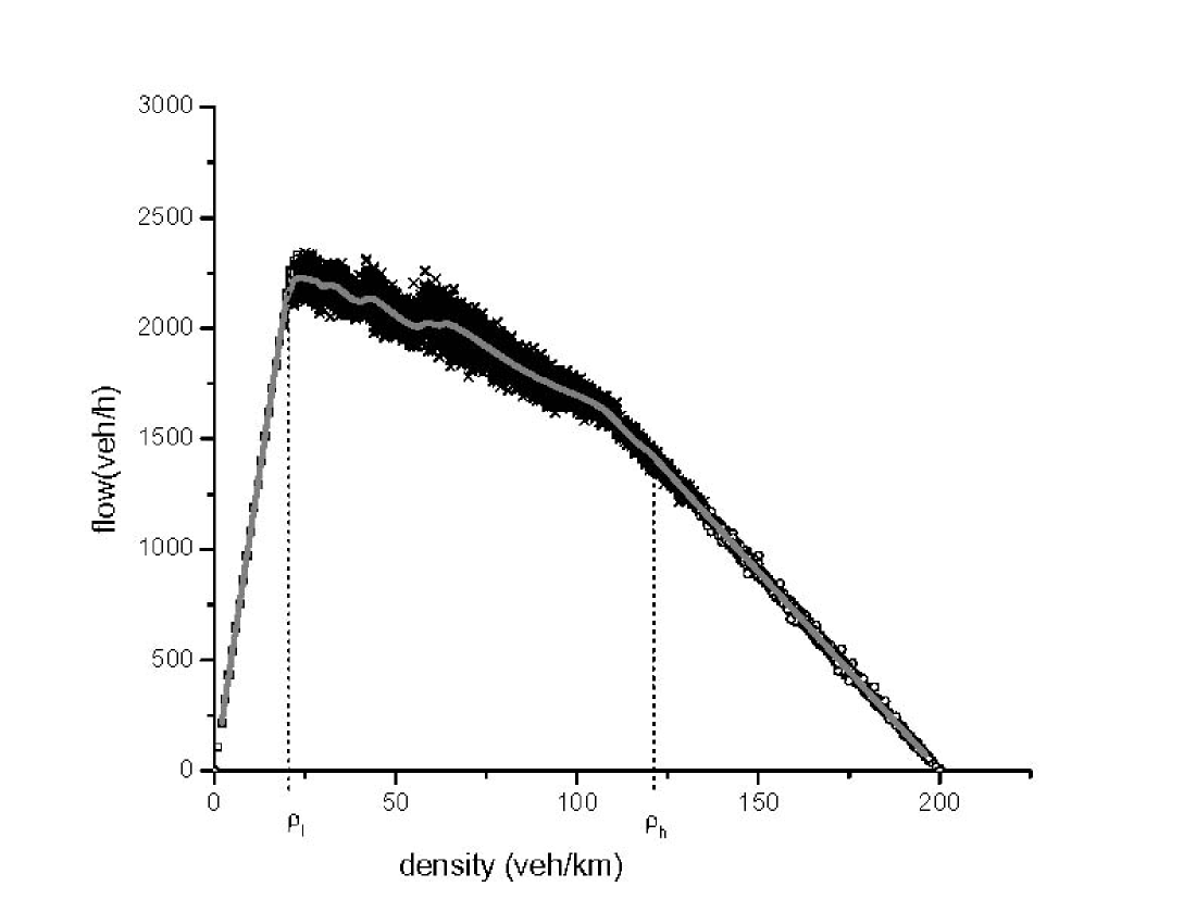
Figure 3: Fundamental diagram resulting from random initial conditions. The simulations are performed on a ring with a length of 20000 cells, each corresponding to $2.5\ m$. The parameters of the model are $v_{max}=108$ $km\ h^{-1}=12\ cells\ s^{-1}$, $R=0.15$, $\Delta x=2.5\ m$, and $M=2$

The next step was to investigate the influence of the probability of random braking $R$ on the simulation results. Figure 2 shows the average fundamental diagram for different values of the parameter $R$. As can be noted from this figure, for very small values of $R$ there are oscillations in the fundamental diagram that are induced by the integer arithmetic. When $R$ reaches a value of $0.10$ these oscillations almost disappear. Note that for values of $R$ from $0.10$ to $0.20$ there is almost no change observed in the fundamental diagram. Thus, value of $R$ was set to $0.15$ for the rest of the simulations presented in this section as with this value there are very small oscillations in the fundamental diagram and the corresponding value of its maximum flow is closer to that reported in the literature for a one lane highway.

3.3 Traffic flow organization

The proposed model is able to reproduce the three states observed in real traffic flow: (i) Free-flow states, which are characterized by a large mean velocity, (ii) synchronized states, where the mean velocity is considerably reduced compared to that of free flow states, but all cars are moving, and (iii) stop-and-go states, where small jams are present. Synchronized traffic and stop-and-go states will be considered as congested states.

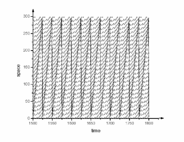
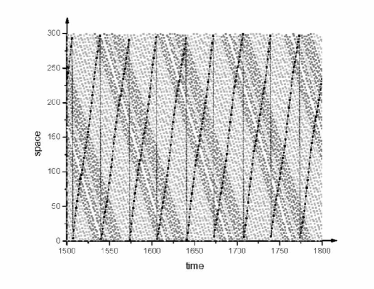
(a)                                   (b)

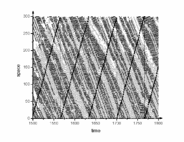
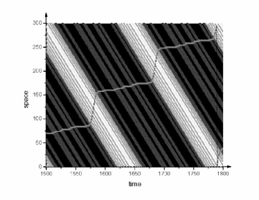
(c)                                   (d)

Figure 4: Time-space diagram for $R=0.15$, $\Delta x=2.5\ m$ and different values of density. The solid lines in diagrams correspond to the trajectory for a specific car at different time-steps. (a) corresponds to a low density range, for $\rho=16\ veh/km$. (b)-(c) correspond to a intermediate density range for $\rho=30$ and $\rho=50\ veh/km$, respectively. (d) corresponds to $\rho=140\ veh/km$

In figure 3, a fundamental diagram obtained from random initial conditions for parameters values of $R=0.15$ and $\Delta x=2.5\ m$ is shown. Each dot in the plot represents a measurement taken by the local flow detector described in the previous section. The white lane is the average flow during all the simulation. One can distinguish, in the fundamental diagram, three different states depending on the global density, namely low density range, high density range and intermediate range for $\rho_{l}<\rho<\rho_{h}$. By increasing $\rho$ in this intermediate range, the flow presents a slow decrease. The explanation for this behavior is related to the fact that according to rule $R4$ of the proposed model drivers can decelerate in more than one unit. In this intermediate range, increasing the number of vehicles leads to relative distances that imply deceleration $d_{dec_{n}}$ to be smaller than the average space gap between two vehicles, $\frac{L}{N}-s$. This forces rule $R4$ to be applied (emergency braking). Vehicles that perform emergency braking produce an instantaneous block of the system and induce other vehicles to reduced their velocities. This causes a local decrease in flow.

The shock waves and jams formations for these three flow regimes can be observed in time-space plots shown in figure 4. The time-space diagram is a graph that describes the relationship between the location of vehicles in a traffic stream and the time as the vehicles progress along the highway. In this figure, each vertical rows of dots represents the instantaneous positions of the vehicles moving towards the right of highway (top), while horizontal rows are vehicles crossing the same highway positions at different time-steps. Trajectories of individual vehicles move forward time and space. One can observe the shock waves and jams formations. For the low density range, these formations are moving forward (see figure 4(a)). After this range, the shock waves move backward (see figures 4(b)-(d)), indicating the presence of congested states. Note that stopped cars with zero velocity only are presented in high density ranges (see figure 4(d)).

As it can be observed in velocity distribution shown in figure 5, for the intermediate density range, vehicles’ velocity is considerably reduced when compared to the low density range, although all vehicles are moving, the situation represents a synchronized state. This figure also allows for a clear distinction between the free flow and the congested state. In the former the mean velocity remains constant at a high value ($v_{max}$), as density increases, a capacity drop occurs resulting in a steady declination of flow (thick solid line). Note that at the critical density, the standard deviation (thin solid line) jumps steeply; this means that vehicles’ velocities start fluctuating after the transition point. Once a compact jam is formed (after $\rho_{h}$), the dominating speed quickly becomes zero.

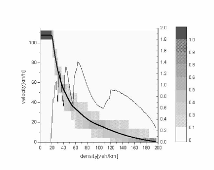
Figure 5: The distribution of vehicles’ speeds, as a function of the global density resulting of the proposed model with $R=0.15$ and $\Delta x=2.5$ $m$. The thick solid line denoted the space mean speed, whereas the thin solid line shows its standard deviation. The gray regions denote the probability density.

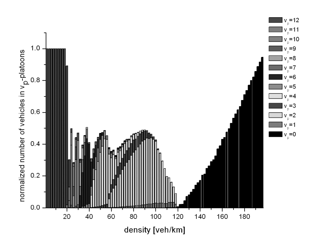
Figure 6: Mean number of vehicles by platoon with velocity $v_{p}$ respect to the mean density

Figure 6 shows the results of a simulation with the same conditions, $R=0.15$ and $\Delta x=2.5$ $m$, as previous figures. In this case the emphasis is in platoon organization. Ordinates in figure 6 show the proportion of vehicles that are traveling in $v_{p}$-platoons. Here $v_{p}$-platoons are defined as a group of two or more neighbor vehicles traveling at the same speed, $v_{p}$, with the space between them dictated by rules $R1$-$R4$. Figure 6 shows that for low densities all vehicles travel at maximum speed and therefore a single platoon is formed. For intermediate densities, there is a reduction in the number of vehicles that are traveling in platoons, although the total number is still significative, as about $40\%$ of vehicles still travel in platoons. When density approaches the stop-and-go values, there is a marked drop in the number of vehicles traveling in platoons, due to an increase in the dispersion of velocities (see figure 5). Finally, for very large densities, the number of vehicles in platoons increases as more and more vehicles have zero velocity. The gray levels in figure 6 are related with an specific velocity, according to the scale showed in its right hand side. It is interesting to note that vehicles traveling as platoons have very similar velocities.

On the other hand, the proposed model in this paper is dependent on the initial conditions. In the next subsection this behavior is analyzed.

3.4 Effects of the initial conditions

In figure 7 two curves for the fundamental diagram for $R=0$ in the range of densities of the interest are shown. The upper curve is calculated by starting from an a homogeneous state, where vehicles are distributed equidistantly with the same initial gap, ($g_{ini}$), and velocity ($v_{ini}$); such that $g_{ini}=\frac{L}{N}-s$ and $v_{ini}$ is equal to the maximal speed such that $g_{ini}\geq d_{keep}$. As opposed to the previous case, to obtain the lower branch the system was initialized by distributing the vehicles with random velocities and positions over the lattice and allowing the system to relax as time pass.

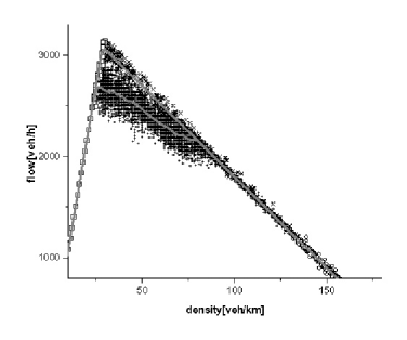
Figure 7: Fundamental diagram resulting from two different initial conditions for $R=0$. The upper curve was calculated by starting from an homogeneous state, whereas the lower curve was obtained from random initial distribution

If system is initialized randomly, this has the effect that some vehicles are spaced more closely to each other. As a direct consequence of this, all vehicles should adjust their velocities according to rules $R3-R4$. In the extreme case, a single vehicle with $v_{n}=1$ $cell/s$ will cause that other vehicles behind apply emergency braking, resulting in total flow decrease shown in the lower curve in figure 7. When, the system is initialized homogeneously with the same gap and velocity for all vehicles, then between the densities $\rho_{1}$ and $\rho_{2}$ a metastable high-flow branch exists. This is due to the fact that for these range of densities the average flow still depends on the initial configuration. For densities just below $\rho_{max}$ the initial gap, $gap_{ini}$, allows to keep the maximum initial velocity equal to $v_{max}$ ($gap_{ini}\geq d\prime_{keep}$, where $d\prime_{keep}$ is the minimum safety distance that should exist between two vehicles to keep the maximum velocity $v_{max}$). After $\rho_{max}$, vehicles can not keep the maximum velocity according to their initial gap and the flow begins to decrease although at a slower pace than that corresponding to a random initialization.

Since $gap_{ini}=L/N-s$, the critical density $\rho_{max}$ where the transition between the free flow and congested state occurs can be calculated as:

$$\rho_{max}=\frac{L}{v_{max}+s}$$

By considering, $\Delta x=2.5\ m$, $s=2$ and setting $v_{max}=12$ $cell/s$ (this equal $108\ km/k$), $\rho_{max}=28.57$ $veh/km$. The associated maximum flow is $q_{max}=\rho_{max}\cdot v_{max}=3085$ $veh/km$. These values are in according to the simulation results shown in figure 7.

4 Summary and conclusions

In this paper a modification of the NaSch model to better capture driver reactions to traffic that are intended to preserve safety on the highway was introduced and investigated. As a result, three distances that represent the safety distance that a driver must have with respect to preceding vehicle if it is going to decelerate, keep its velocity or accelerate, were included in the new model. The addition of these distances allowed to determine the most appropriate action for a vehicle to undertake based on the distance from the vehicle ahead of it and the velocities of the two neighbor vehicles. In this way, the velocity setting rules depend not only on the relative velocity of neighbor vehicles, they now take into account their relative distance. With this modification the normal drivers behavior that bases their driving decisions on both relative velocity and relative distance was incorporated. The determination of safe distances is in accordance with normal drivers spacing policies, for example, those based on vehicle following, constant time headway, etc. Moreover, acceleration and deceleration magnitudes for basic maneuvers are used here are much closer to those reported for normal driving. It is important to emphasize that the order for applying rules $R1$ to $R4$ of the proposed model, is not relevant as conditions for each one form disjoint sets. Besides, in the model here proposed randomization is applied only to vehicles that are in cruising conditions and do not require to brake. In this way double braking is avoided, this is consistent with the idea of treating random braking as a disturbance that should not occur very often.

The new model was tested by extended simulations on a one-lane highway with a ring topology. The effect of several critical model parameters was analyzed: cell lengths, random braking level and initial conditions with the intention of finding values that would lead to a proper representation or real traffic behavior. Simulation results proved that this new model properly reproduced real traffic flow phenomena. Results obtained for homogeneous drivers and different cell lengths exhibit the three states observed in real traffic flow: Free-flow states, synchronized states, and stop-and-go states, where small jams are present. Synchronized states are associated to intermediate-levels of density where vehicles move with a velocity lower than the corresponding to free-flow and all vehicles are moving. In this way, stopped cars with zero velocity are only present in high density ranges.

On the other hand, simulation results for $R=0.15$ and $\Delta x=2.5$ $m$, exhibit groups of two or more neighbor vehicles traveling at the same speed with the space between them dictated by rules $R1$-$R4$ (platoons). For intermediate densities, where the synchronized states exist, the number of vehicles that are traveling in platoons is about $40\%$. The platoon formation observed plays an important role in both automated and non-automated highway systems. Therefore, results obtained can help to elucidate the effects of anticipation coded in the safe distances and the length of cell. Besides, the influence of the variation of speed on the flow is also found to be a factor of great importance in traffic synchronization.

Summarizing, the results and discussions in this paper showed the flexibility of the CA approach to more complex traffic flow problems. A simple and natural modification of the rules of the NaSch model to better capture driver reactions allowed to describe the three states of flow observed in the reality. Moreover, the model still preserved simplicity of CA model and at the same time, as vehicles’ behavior was based on a safety analysis to determine the most appropriate action for a vehicle to take, made results closer to real highway behavior. Besides, there is an intuitive explanation for all rules in the model. It is important to remark that although in this paper the model is simulated in a single-lane on a ring, it is possible to apply it to complex highway topologies in a satisfactory way. Work in this direction is currently in progress.

References

References

- [1] Wahle J, Neubert L, Esser J and Schreckenberg M 2001 Parallel Comp. 27 719
- [2] Autobahn Project North Rhine-Westphalia. Available at http://www.ptt.uni-duisburg.de/en/projekte/babnrw/
- [3] Schadschneider A, Knospe W, Santen L and Schreckenberg M 2005 Physica A 346–1–2 165–173.
- [4] Nagel K and Schreckenberg M 1992 Phys. I 2 22221–2229.
- [5] Knospe W, Santen L, Schadschneider A, and Schreckenberg M 2000 J. Phys. A: Math. Gen., 33 477–485.
- [6] Lárraga M E, del Río J A , and Schadschneider A 2004 J. Phys. A: Math. Gen. 37(12) 3769–3781.
- [7] Lárraga M E, del Río J A, and Alvarez L 2005 Transp. Res. C, Emerg. Technol 5 63–74.
- [8] Esser J and Schreckenberg M 1997 Int. J. Mod. Phys. C 8 1025 -1036.
- [9] Hafstein S F, Chrobok R, Pottmeier A, Schreckenberg M, and Mazur F 2004 Computer-Aided Civil and Infrastructure Engineering, 19–5 338–350.
- [10] Rickert M. and Wagner P 1996 Int. J. of Mod. Phys. C 7 133–153
- [11] Schreckenberg M, Neubert L, and Wahle J 2001 Future Generation Computer Systems, 17 649–657.
- [12] Alvarez L. and Horowitz R 1999 Veh. Sys. Dyns., 32–1 23–56.
- [13] Godbole D. and Lygeros J 1994 IEEE Trans. on Veh. Tech., 43–4 1125–1135.
- [14] Carbaugh J, Godbole D N, and Sengupta R 1997 Proc of the ACC
- [15] Hitchcock A 1993 Technical Report PATH Memorandum 93-9, Institute of Transportation Studies, University of California, Berkeley, .
- [16] Lygeros J, Godbole D N, and Broucke M 2000 IEEE Trans. Cont. Syst. Tech.8 205–219.
- [17] Broucke M. and Varaiya P 1996 Transp. Res. C, Emerg. Technol 3 181–210.