Cycles in Nonlinear Macroeconomics

’All linear systems are equally happy, whereas each nonlinear system is unhappy in its own way.’

Yu. Bolotin, A. Tur, and V. Yanovskii

”Constructive Chaos”

Preface

Nonlinear dynamics is one of the most important and prospective trends of the development of economic science. Powerful modern techniques of qualitative theory of differential equations and related subjects of mathematical topology provide broad possibilities of obtaining substantial results of qualitative character, in the first place, in solving the problems of economic forecasting. Mathematical economics is characterized by two principally different ways of modeling, i.e., static and dynamic ones. Following N. D. Kondratev [25], we shall dwell on a more detailed and concrete characterization of these two purely theoretical approaches to the study of economic reality.

The static theory considers economic processes in terms of their instant manifestation, without any regard to inertial changes in time. The static approach to the modeling of economic reality is based on the concept of the equilibrium of interrelated elements of an economic system. The concept of equilibrium itself had been sufficiently well familiar to scientists concerned with mechanics before the appearance in 1776 of Adam Smith’s prominent work ”An Inquiry into the Nature and Causes of the Wealth of Nations” wherein, as it seems, the author managed to find an analogy between the economic balance and the resultant force in mechanics. A. Smith put forward the most substantial postulate of the general theory of equilibrium: namely, an ability of the system of competition to achieve such a distribution of resources that, in a sense, proves to be efficient.

On positions analogous to those of A. Smith stand also the constructions of D. Ricardo who put forward the thesis of the freedom of competition and the freedom of movement of labor and capital from one sphere of economic relations to another. D. Ricardo was aware of the fact that the actual price, the actual level of wages and incomes are variables with respect to time, and, at that, he suggested that there exist a tendency towards attaining a certain natural level of equilibrium for the above mentioned characteristics.

An exhaustive formulation of the general concept of equilibrium rightfully belongs to L. Walras, a representative of the school of marginalism (or marginal utility). Works by L. Walras, S. Jevons, and V. Pareto unified the theory of equilibrium with regard to an application to the spheres of exchange, production, capital and money. They were subsequently elaborated by J. Hicks and P. Samuelson. On the whole, these works are of rather broad, comprehensive character: economy is considered as a set of individual consumers and producers, and the number of involved variables is absolutely unlimited. The system of general equilibrium is closed in the sense that the whole set of variables is determined by given conditions. In order to verify the compatibility of the system with the state of equilibrium, one only has to compare the number of equations with the number of unknown variables. However, there exists the problem of the existence of the point of equilibrium and of its uniqueness.

The dynamic analysis in economics formed in parallel with economic theory itself. A confrontation between the dynamic and static approaches can be easily traced throughout the whole history of the economic thought. Apparently, the reason lies in principal differences between the understanding of the balance of the equilibrium of forces and casual dynamics. There is a vast choice of literature references concerned with the theory of economic dynamics. Among a large number of different problems of evolutionary economics, the problems of economic growth and of business cycles are the most important ones. In the treatment of N. D. Kondratev, these distinctions between dynamic processes are interpreted as evolutionary (nonrecurrent, irreversible) and wave-like (recurrent, reversible). By evolutionary (or irreversible) processes one means those changes that in the absence of external perturbative interactions flow in a certain, one and the same, direction. Examples of such processes are given by tendencies of population growth, increase in the total volume of production, etc. N. D. Kondratev terms as wave-like (or reversible) those processes of changes that at each point in time have their specific direction and, consequently, change it permanently. In these processes, the phenomenon, being at a given moment in a given state and changing it afterwards, sooner or later may return to the initial state. The processes of changes in the prices of different consumer goods, interest rates, the level of unemployment, etc. may serve as examples.

In our view, more attention should be paid to the issue of slow (low-frequency) oscillations in economics, i.e., to the so-called long cycles (waves). N. D. Kondratev himself, while singling out long waves of economic activities, related them to the industrial revolution at the end of the XVIIIth - beginning of the XIXth centuries, the construction of railway networks, the dissemination of new communication means (telephone, telegraph) and of electric power, as well as rapid development of automotive industry [2]. Nowadays, the most wide-spread concept is that of five long cycles whose length is approximately equal to 50 years:

• the end of the XVIIIth century - the first third of the XIXth century;

• the second third of the XIXth century - the early 90s of the XIXth century;

• the end of the XIXth century - the 30s of the XXth century;

• the 40s of the XXth century - the 70s of the XXth century;

• from the 80s of the XXth century up to the present time.

Let us try to understand the very nature of the mechanism of the long cycle. To initiate the expansion phase of the cycle, it is necessary to accumulate not only inventions but also capital as well as a desire of entrepreneurs to increase investments. For the industrialist, the dynamics of profit is a factor of primary importance. As a matter of fact, the expansion wave of the long cycle develops as a system of mutually related and mutually stimulating phenomena: an innovation provides a possibility to improve the production conditions, to reduce production costs and to increase profit, which stimulates entrepreneurs to introduce innovations under the condition of availability of necessary resources. Innovations give rise to an increase in profit, which generates additional investments, an increase in the volume of demand and a general positive movement of the growth rate of business factors.

However, at a certain moment the dynamics of the process exhibits a return point. A technological basis for this is provided by substantial weakening of the factors that initiated the expansion phase of the cycle. A cessation of their action slows down the growth of profitability and then decreases it, which reduces the interest of business structures in further innovations and investments. The industry slows down its growth, and negative effects of the economic life, typical of long-wave decline, appear. In the process of this decline, an increase in the number of new inventions takes place, which creates a prerequisite for the completion of the decline and the beginning of a new expansion wave.

N. D. Kondratev’s undoubted merit consists in the fact that he based his conclusions on an analysis of long temporal series of prices of the commodity output, of interest rates, wages, etc. The above-described dynamics is merely a simplified scheme, because the actual changes in the economy are much more complicated and diverse.

The modern status of macroeconomics cannot be understood without an evaluation of the contribution of J. M. Keynes. As a matter of fact , he created macroeconomics as a science in the 1930’s in order to explain the causes of the Great Depression that proved to be the most large-scale recession of the XXth century and, as such, the most important event in the modern history of business cycles [18]. The theory, existing at that time, could not explain why the GDP of the USA had fallen by one third from 1929 to 1933 and the unemployment level had risen to one fourth of the total work force. The classical theories were bases on the assumption that the economy was at competitive equilibrium, with the market regulating everything. In particular, high unemployment had to give rise to the reduction in wage rates down to the level where the employers would agree to employ all those who were willing to work for these wages and unemployment would disappear by itself. However, in practice, this was not the case. Therefore, Keynes put forward radically new ideas whose essence could be reduced to two major postulates.

Firstly, the economy is not at competitive equilibrium at each separate moment; that is, the ”invisible hand” of the market does not fulfil its duties. The basic reason for this equilibrium is the conservation of fixed prices and wage rates for a long time and the absence of adaptation to the current market conditions. Secondly, the level of the development of the economy is determined by the aggregate demand, and the latter, in its turn, depends on some unexplained factors that were vaguely termed by Keynes as ”the brute of investors”. On the basis of these two assumptions, the edifice of the theory of macroeconomics was erected. According to its postulate, the volume of the GDP of the country is influenced by the scale of expenditure of consumers, investors and the government on commodities and services. Therefore, business cycles are stipulated exactly by oscillations of the demand rather than by resources of the country. The first and main formal Keynesian model IS-LM was formulated on the basis of the Keynesian theory by J. Hicks in 1937.

In the course of the next several decades, up to the mid-70s, the discussion went on mostly in the mainstream of the Keynesian theory. The issue was whether the government should at all try to revive the economy in the periods of decline and, if it were so, by what means. According to the above-mentioned position, the government had to react to the decline by increasing government spending. From a point of view of other scientists and specialists, stabilization should be achieved by means of control over money supply: this point of view gave rise to the development of the doctrine of monetarism according to which the main objective of the state is to avoid strong oscillations of the money supply. Nevertheless, the positions of both the antagonistic scientific trends agreed on the point that the basis driving force of the cycle were oscillations of the volume of demand, and, therefore, the main differences between ”Keynesians” and ”monetarists” were almost completely obliterated.

However, in the mid-1970s the word economy faced a new phenomenon, i.e., stagflation, that could not be satisfactorily explained within the framework of the Keynesian concept. At that time, there appeared critical works of R. Lucas, subsequently the 1995 Nobel Prize winner, who criticized not only the economic policy of the authorities but also the whole Keynesian theory of business cycles for the disregard of optimum behavior of business agents including the formation of rational expectations. He suggested that, in contrast to investors and consumers in Keynes’s models that followed certain formal rules of behavior, business agents made, on the average, correct forecasts of the future state of the economy and adhered to the strategy of maximizing their own profits. All this created a demand for some alternative theory of business cycles.

This niche was occupied by the American economists F. Kydland and E. Prescott, who won the 2004 Nobel Prize for Economics. In their seminal paper [45], they proposed a new description of a real business cycle based on the fact that firms maximized the profit and made decisions to invest taking into account the expectation of future demand for their product and of the development of technologies.

Kydland and Prescott presented a series of dynamic models and showed what kind of behavior of basic economic variables (GDP, investment, and savings) was to be expected depending on the effect of technological shocks upon labour productivity and changes in external market conditions. The authors demonstrated that the results of modelling were in satisfactory agreement with the observed regularities. Besides, they drew an important conclusion that a considerable part of oscillations of GDP in many countries corresponded to the predictions of equilibrium models. In other words, there is no need to introduce into these models deviations from market equilibrium in the Keynesian spirit and to realize governmental stabilization policy.

For fairness, it should be noted that the theory of cycles of F. Kydland and E. Prescott by no means explains all the phenomena of actual economic reality: it is permanently subjected to constructive criticism by ”new Keynesianists”. In particular, the most striking example of disagreement between representatives of these two schools is an attempt to explain the technological boom of the 1990s. One is just left with expectations that in not too remote future a consensus will be achieved concerning the actual sources of business cycles.

In our point of view, the achievement of this goal is impossible without accepting the fact that economics, in essence, is a developing system and should be constructed within the framework of the theory of developing systems whose constructiveness is convincingly proved by the example of chemical kinetics, biology and other natural sciences. In this theory, it is shown that in the process of proceeding to the goal in the presence of substantially nonlinear feedback couplings, there emerges a whole hierarchy of instabilities that leads to the appearance of limit cycles, homoclinic structures and  to spontaneous formation of chaos. As a result of such transformations (bifurcations), several different states of business equilibrium may appear (the so-called effect of bistability). The methods of nonlinear mechanics allow us to predict the moment of the occurrence of a chaotic regime in the system under investigation, the number of possible states of equilibrium and to determine the character of their stability. All this, in its turn, generates a principal general problem of the construction of alternative scenarios of complex, irreversibly developing system. It would be in order to mention here the statement of G. Malinetskii [28]: ”Indeed, social-technological objects are complex hierarchy systems, with various processes in them developing at different characteristic time scales. The rate of their instability, the limits of their predictability are different as well. In the economic system, the horizon of the forecast has fallen sharply: whereas just 15 years ago 5-year directive or indicative planning was a norm in the world, nowadays this is out of question. In the world, there is more and more supply of ’quick money’ and less and less supply of ’slow money’. However, on the other hand, stable development of the society requires slowly changing strategic goals, scales of social values and norms, culture and ideology. One needs technique, theory and formalism that would allow one to analyze possible dynamics of such ’different-time-scale’ systems and to direct their development on this basis.”

One can hardly question the fact that exactly the mathematical technique of nonlinear dynamics provides the very tools that allow us to approach closely the solution of the problem of ”designing the future”, of finding stable and safe ways of social and economic evolution. The experience of the application of methods and models of nonlinear dynamics has shown that many complex developing systems can be satisfactorily described with the help of a small number of variables, the order parameters. The determination of the order parameters is realized by reduction of the multidimensional system to a subspace of a small dimension owing to methods of the theory of bifurcations and of the theory of central manifolds. However, exactly this fact predetermines the locality of the carried out analysis of dynamic behavior of the studied system. Its applicability is admissible only in small neighborhood of the bifurcation point, to solutions of small amplitude. In what follows, we shall present other periodic solutions of small amplitude generated as a result of the Andronov-Hopf bifurcation of limit cycles and shall determine the character of their stability.

In this book, the choice of the discussed models is made more or less arbitrarily. The authors consider the models that are rooted in basic principles of traditional economics, neoclassical synthesis and Keynesianism.

Chapter 1 Instability and cycles in the Walras-Marshall model

Economics operates such notions as the quantity of goods (productive factors) and their price. In every market, there exist groups of sellers and buyers. In this chapter, a model of the market for one kind of goods will be considered. In the model of a single market the variables, i.e., functions of time, are the volumes of bought and sold goods as well as their prices. The basic principle of modeling of the market interaction is the formation of balance relations between the volumes of the demand and the supply of goods and, accordingly, the prices of the demand and the supply.

The problem of joint action of demand and supply as indicators determining quantitative relations between the volume of a commodity and its price in a given market is very precisely characterized by A. Marshall [29]: ”We could ask on equal grounds whether the price is regulated by utility or production costs, or whether a sheet of paper is cut by the upper or the lower blade of the scissors. Indeed, if one blade is kept motionless and cutting is carried out by the motion of the other blade, we can, without a good deal of thinking, argue that cutting is done by the second blade. However, such an argument is not completely exact, and it may be justified only by a pretension to mere popularity rather than to an exact scientific description of the realized process.”

For more concrete understanding of the modern phenomenological basis of demand and supply, we should  present a definition of these notions, using the formulations given, e.g., in [16].

By the commodity demand one means the quantity of this commodity that an individual, a group of individuals or the population on the whole are ready to buy per unit time under certain conditions. A list of these conditions includes the tastes and the preferences of the buyers, the price of this commodity, the income rate, etc. By the demand price one means the maximum price the buyers agree to pay for a fixed quantity of a given commodity. At the same time, the dependence of the volume of the demand on its determining factors is called the demand function.

Analogously, the supply serves as a characteristic of the readiness of the seller to sell a certain quantity of the commodity in a fixed period of time.

By the volume of the supply one means the quantity of a certain commodity that one seller or a group of sellers are willing to sell in the market per unit time under certain conditions.

These conditions, as a rule, include the properties of the applied manufacturing technology, the price of the given commodity, the price rates of the employed resources, tax rates, subventions, etc. The supply price is the minimum price at which the seller agrees to sell a certain quantity of a given commodity. The dependence of the volume of the supply on the structure of its determining factors is called the supply function.  Let us point out that the supply function as well as the demand function can be represented in three ways: in the form of numerical tables, graphically, and analytically. In what follows, we shall use only analytical representations for the functions of the demand and the supply.

1.1 Nonlinearity in the Walras model

In classical economic theory, one employs two equally admissible but principally different versions of the description of the mechanism of an interaction between the demand and the supply. The first approach, worked out by L. Walras, postulates that the driving force of changes in the price is the volume of excess demand under a given instant value of the price. In a dynamic aspect, the process of finding the equilibrium in L. Walras’s spirit can be represented in the form of the differential equation

$$\frac{dP}{dt}=m\left(Y^{D}\left(P\right)-Y^{S}\left(P\right)\right),$$ (1.1)

where $P=P\left(t\right)$ is the price of the commodity;

$Y^{D}=Y^{D}\left(P\right)$ is the volume of the demand;

$Y^{S}=Y^{S}\left(P\right)$ is the volume of the supply;

$m>0$ is a constant of the time of the limit process;

$t$ is time.

The sign of the quantity $\Delta Y=Y^{D}-Y^{S}$, called the volume of excess demand, determines the direction of the changes in the price. It is obvious that for $\Delta Y>0$ the market price rises, whereas for $\Delta Y<0$ it falls. The condition of the existence of an equilibrium price $P_{E}$ is the existence of the solution to the equation

$$Y^{D}\left(P_{E}\right)-Y^{S}\left(P_{E}\right)=0.$$ (1.2)

There exists also a different approach to the problem under consideration, attributed to A. Marshall. Its essence is that a change of the volume of the mass of commodities in a given market is determined by the influence of the difference between the demand price and the supply price, to which the sellers (or the manufacturers) respond by an increase or a decrease in the volume of the supply of the commodity. In a mathematical form, this statement is expressed by means of the following differential equation:

$$\frac{dP}{dt}=m\left(P^{D}\left(Y\right)-P^{S}\left(Y\right)\right),$$ (1.3)

where $Y=Y\left(t\right)$ is the volume of the commodity;

$P^{D}\left(Y\right)$ is the demand price;

$P^{S}\left(Y\right)$ is the supply price;

$m>0$ is a time constant.

In Eq. (1.3), a surplus of the demand price over the supply price stimulates an increase in $Y$; and if the supply price is higher than the demand price, the value of $Y$ decreases. An equilibrium value of the volume of the commodity $Y_{E}$ is determined from the equation

$$P^{D}\left(Y\right)-P^{S}\left(Y\right)=0.$$ (1.4)

The algebraic equations (1.2) and (1.3) may have only one or several solutions. It means that both a unique state of equilibrium as well as a set of equilibrium states is possible. It is obvious that the nonuniqueness of equilibrium values of the volume and of the price of the commodity is explained by the presence of nonlinear relations in the basic equations.

An important problem is an analysis of the stability of the available states of equilibrium. It is necessary to ascertain the reasons why an equilibrium volume of the market remains constant under certain, remaining within certain limit values, fluctuations of the price, or on the other hand, why, under a given equilibrium price rate, changes in the volume of the commodity also take place. In what follows, by the stability of equilibrium we understand an ability of the overbalanced market to return again to the initial state owing to the action of endogenous factors. Besides, the problem of the stability of market equilibrium is directly related with the problem of the necessity to employ additional measures to regulate market relations.

First of all, let us consider the problem of stability of the economic model (1.1) described L. Walras’s theory. Let us set the coefficient $m=1$ in Eq. (1.1). In the neighborhood of the equilibrium point $P=P_{E}$ determined by the solution of Eq. (1.2), we can approximately represent the functions of the demand $Y^{D}\left(P\right)$ and of the supply $Y^{S}\left(P\right)$ in the form of polynomials obtained by the truncation of the corresponding Taylor series

$$Y^{D}\left(P\right)\approx\sum_{i=0}^{k}\frac{d_{i}}{i!}\left(P-P_{E}\right)^{i},\quad Y^{S}\left(P\right)\approx\sum_{i=0}^{k}\frac{S_{i}}{i!}\left(P-P_{E}\right)^{i},$$ (1.5)

$$d_{i}=\frac{d^{i}Y^{D}\left(P_{E}\right)}{dP^{i}},\quad S_{i}=\frac{d^{i}Y^{S}\left(P_{E}\right)}{dP^{i}},\quad i=\overline{0,k}.$$

If we introduce a new variable $x=P-P_{E}$, which is a deviation of the price from its equilibrium value, equation (1.1) takes the form

$$\dot{x}=F_{k}\left(x\right),$$ (1.6)

where $\dot{x}=\frac{dx}{dt}$, $F_{k}\left(x\right)=\sum_{i=0}^{k}\frac{a_{i}}{i!}x^{i}$, $a_{i}=d_{i}-S_{i}$. Note that from (1.2) it follows $a_{0}=0$, because $d_{0}=S_{0}=Y_{E}$, which is an equilibrium volume of the market. At the same time, $x=0$ is a stationary point (the state of equilibrium) of Eq. (1.6).

The differential equation (1.6) is called a dynamic system of the first order. The phase space of the considered system is one-dimensional, therefore, the studied process of change in the price can be represented by the motion of an image point on the phase straight [8].

Indeed, in general, the main elements that determine the partition of the phase straight into trajectories are the states of equilibrium of the system. The values $x=x_{j}$ that make the function $F_{k}\left(x\right)$ vanish are themselves independent phase trajectories. The rest of the trajectories consist of line segments between the roots of the equation $F_{k}\left(x\right)=0$, or of rays forming half-intervals between one of the roots and infinity. The direction of the motion of the image point along these trajectories is determined by the sign of the function $F_{k}\left(x\right)$: for $F_{k}\left(x\right)>0$ the image point moves to the right, whereas for $F_{k}\left(x\right)<0$ it moves to the left. If the form of the curve $z=F_{k}\left(x\right)$ is known, it is not difficult to establish concrete partition of the phase straight into trajectories.

An example of such partition is given in Fig. 1.1, where the arrows show the direction of the motion of the image point. From the structure of the partition of the phase straight into trajectories, it follows directly that the states of equilibrium of the system at the points $x_{1}$, $x_{4}$ are stable, whereas they are unstable at the points $x_{2}$, $x_{3}$, $x_{5}$. It is directly seen in Fig. 1.1 that in the stable states of equilibrium the derivative $F_{k}^{\prime}\left(x\right)<0$, whereas in the unstable states $F_{k}^{\prime}\left(x\right)>0$. The value $F_{k}^{\prime}\left(x\right)=0$ may occur at points of both the stable and unstable state of equilibrium. (This situation itself deserves independent consideration, because it requires some additional conditions for the determination of the type of stability of the stationary point.)

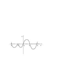
Figure 1.1: The dependence of the excess-demand function on price deviations.

As the character of the change of the variable in the first-order system (1.6) is completely determined by the explicit form of the function $F_{k}\left(x\right)$, it is of interest to consider cases of different values of the order of the polynomial $k$.

Let $k=1$. Then $F_{1}\left(x\right)=a_{1}x$ is a linear function, and there exists the single state of equilibrium $x_{E}=0$. The stability condition in this case is $F_{1}^{\prime}\left(0\right)<0$. This inequality reduces to the relation $d_{1}<S_{1}$ which is the classical condition of stability of L. Walras.

Let us try to interpret the linear stability of L. Walras using the notion of the elasticity of the demand and supply functions to price.

According to the definition of elasticity, in our notation, we have:

$$\eta_{D}=\frac{d_{1}P_{E}}{d_{0}},\quad\eta_{S}=\frac{S_{1}P_{E}}{S_{0}},$$

or, taking into account that $d_{0}=S_{0}=Y_{E}$,

$$\eta_{D}=\frac{d_{1}P_{E}}{Y_{E}},\quad\eta_{S}=\frac{S_{1}P_{E}}{Y_{E}},$$ (1.7)

where $\eta_{D}$, $\eta_{S}$ are coefficients of the demand and supply elasticities to price. They are dimensionless, i.e., relative, quantities.

Therefore, the inequality $a_{1}=d_{1}-S_{1}<0$ can be easily reduced to the form

$$a_{1}=\frac{Y_{E}}{P_{E}}\left(\eta_{D}-\eta_{S}\right)<0.$$ (1.8)

Given that $Y_{E}$, $P_{E}$ are always positive, the condition of L. Walras is formulated as follows: for the stability of the linear system (1.6) with $k=1$, it is necessary that the elasticity of the volume of the supply to price should exceed the corresponding demand elasticity, i.e., $\eta_{S}>\eta_{D}$. In other words, if we introduce the quantity $\eta=\eta_{D}-\eta_{S}$ conditionally termed an excess-demand elasticity to price, the stability of (1.6) is determined by the sign of $\eta$: for $\eta<0$, we have stability, and, on the contrary, for $\eta>0$, we have instability.

Let us consider the peculiarities of the behavior of the system (1.6) in the case $k=2$. Here, $F_{2}\left(x\right)=a_{1}x+\frac{a_{2}}{2}x^{2}$ is a quadratic function of the initial variable.

The equation $F_{2}\left(x\right)=0$, or $a_{1}x+\frac{a_{2}}{2}x^{2}=0$, has two roots: $x_{E}^{1}=0$ and $x_{E}^{2}=-\frac{2a_{1}}{a_{2}}$. To determine the character of stability of each singular point, it is necessary to evaluate $F_{2}^{\prime}\left(x_{E}\right)$.

As a result of differentiation, we have:

$$F_{2}^{\prime}\left(x_{E}\right)=a_{1}+a_{2}x_{E}\text{.}$$ (1.9)

The substitution of the values of $x_{E}^{1}$ and $x_{E}^{2}$ in expression (1.9) yields

$$F_{2}^{\prime}\left(0\right)=a_{1}\text{,\quad}F_{2}^{\prime}\left(-\frac{2a_{1}}{a_{2}}\right)=-a_{1}.$$

It is thus obvious that the stability of both the states of equilibrium is completely characterized by the sign of the quantity $a_{1}$ (or $\eta$).

In this case, if $a_{1}>0$, i.e., if the demand is more elastic than the supply, the state of equilibrium $x_{E}^{1}=0$ is unstable, whereas $x_{E}^{2}=-\frac{2a_{1}}{a_{2}}$ is stable.

Figure 1.2: The diagram of the transcritical bifurcation.

On the contrary, for $a_{1}<0$ (the demand is less elastic than the supply), $x_{E}^{1}$ is a stable state of equilibrium, and, accordingly, $x_{E}^{2}$ is an unstable one.

In a noncoarse situation, when $a_{1}$ is a small quantity changing its sign in the neighborhood of zero, the so-called transcritical bifurcation appears illustrating a change of stability of the states of equilibrium: see Fig. 1.2, where $a_{2}<0$.

As a result of this bifurcation, the singular points $x_{E}^{1}$ and $x_{E}^{2}$ merge for $a_{1}=0$, i.e., when the elasticity of the demand is equal to that of the supply, to form the single two-fold state of equilibrium $x_{E}=0$. At the same time, the condition $a_{2}\neq 0$ is important.

Here, we can observe a considerable difference between the behavior of the nonlinear system from that of the linear model, which manifests itself in the present of two equilibrium values that are transformed into one and the same point of equilibrium as a result of a transcritical bifurcation.

It seems to be reasonable to attribute pithy economic meaning to the coefficient of the quadratic term, $a_{2}$, in terms of elasticities of the demand and supply functions. To this end, it is necessary to find the derivatives of the corresponding types of elasticity with respect to the price at the point $P_{E}$. Skipping over intermediate transformations, we present the following expressions for the quantities $d_{2}$ and $S_{2}$ as functions of $\eta_{D}^{\prime}$, $\eta_{S}^{\prime}$, $\eta_{D}$, $\eta_{S}$:

$$d_{2}=\frac{Y_{E}}{P_{E}^{2}}\left(\eta_{D}^{\prime}P_{E}-\eta_{D}+\eta_{D}^{2}\right),$$

$$S_{2}=\frac{Y_{E}}{P_{E}^{2}}\left(\eta_{S}^{\prime}P_{E}-\eta_{S}+\eta_{S}^{2}\right).$$ (1.10)

Subtracting the second equation of (1.10) from the first one, we get

$$a_{2}=\frac{Y_{E}}{P_{E}^{2}}\left(\left(\eta_{D}^{\prime}-\eta_{S}^{\prime}\right)P_{E}+\left(\eta_{D}+\eta_{D}-1\right)\left(\eta_{D}-\eta_{S}\right)\right),$$

or

$$a_{2}=\frac{Y_{E}}{P_{E}^{2}}\left(\eta^{\prime}P_{E}+\left(\eta_{D}+\eta_{D}-1\right)\eta\right).$$ (1.11)

It is worth noting that the dependence of the coefficient $a_{2}$ on the excess-demand elasticity $\eta$ and on its derivative with respect to the price $\eta^{\prime}$ is a linear function.

Let us consider the case when the function of an excess demand in the system (1.6) is cubic. This takes place for $k=3$, and, accordingly,

$$F_{3}\left(x\right)=a_{1}x+\frac{a_{2}}{2}x^{2}+\frac{a_{3}}{6}x^{3}\quad\left(a_{3}\neq 0\right).$$

The cubic equation $F_{3}\left(x\right)=0$ may have, depending on the coefficients, one or three real roots, and, accordingly, the system (1.6) may have one or three states of equilibrium.

By analogy with the previous case, the stability of each state of equilibrium is determined by the sign of $F_{3}\left(x_{E}\right)$.

Let the system (1.6) have the representation

$$\dot{x}=a_{1}x+\frac{a_{2}}{2}x^{2}+\frac{a_{3}}{6}x^{3}.$$ (1.12)

Assuming the parameters $a_{1}$, $a_{2}$ to be small, sign-alternating quantities, we consider the deformation of the saddle-node bifurcation with an additional degeneracy in the quadratic term [4]. In the saddle-node case, the truncated system with $a_{1}=0$, $a_{2}=0$ takes the form

$$\dot{x}=\frac{a_{3}}{6}x^{3}.$$ (1.13)

After some thinking, we can arrive at the conclusion that there exist small perturbations of the function $\frac{a_{3}}{6}x^{3}$ when the system possesses one or three hyperbolic fixed points (the states of equilibrium) in the neighborhood of $x_{E}=0$, as well as certain ”unusual” perturbations when the system possesses two fixed points, with one of them being nonhyperbolic. All the above-mentioned possibilities can be accounted for by adding low-order terms. It is customary to represent this deformation in the form of the equation

$$\dot{u}=\theta_{1}+\theta_{2}u+\frac{a_{3}}{6}u^{3},$$ (1.14)

where $u=x+\frac{a_{2}}{a_{3}}$, $\theta_{1}=\frac{a_{2}}{a_{3}}\left(\frac{a_{2}^{2}}{3a_{3}}-a_{1}\right)$, $\theta_{2}=a_{1}-\frac{a_{2}^{2}}{2a_{3}}$.

Here, $\theta_{1}$, $\theta_{2}$ are also small quantities. The dynamics of this vector field is formed, with the accuracy of topological equivalence, by its fixed points and the types of their stability. Generally speaking, mathematical theory of singularities provides the means for a systematic study of zeros of families of mappings, with one of the examples being given by the right-hand side of Eq. (1.14).

Let us find the bifurcation set of parameters in the parameter plane $\theta_{1}$, $\theta_{2}$ by demanding that the right-hand side of (1.14) and its derivative with respect to the variable $u$ vanish:

$$\psi\left(u\right)=\theta_{1}+\theta_{2}u+\frac{a_{3}}{6}u^{3}=0,$$

$$\psi^{\prime}\left(u\right)=\theta_{2}+\frac{a_{3}}{2}u^{2}=0.$$ (1.15)

By eliminating the variable $u$ from both the equations of the system (1.15), we arrive at the following bifurcation set:

$$8\theta_{2}^{3}+9a_{3}\theta_{1}^{2}=0.$$ (1.16)

The bifurcation diagram of the system (1.14) is presented in Fig. 1.3 for the case $a_{3}<0$. The system (1.14) may possess one or three coarse states of equilibrium. These states of equilibrium merge in pairs on bifurcation lines $G_{1}$ and $G_{2}$ [formula (1.16)] that form Neile’s semicubical parabola with the origin at the point $\mathbf{A}=\left(0,0\right)$. The point $\mathbf{A}$ corresponds to merging of all the three states of equilibrium into one state. For the values of the parameters in the plane $\theta_{1}$, $\theta_{2}$ that lie inside the parabola (region 2), the system (1.14) possesses three states of equilibrium (two stable states and one unstable state in between), whereas for the ”outside” values of the parameters (region 1) there exists one (stable) state of equilibrium.

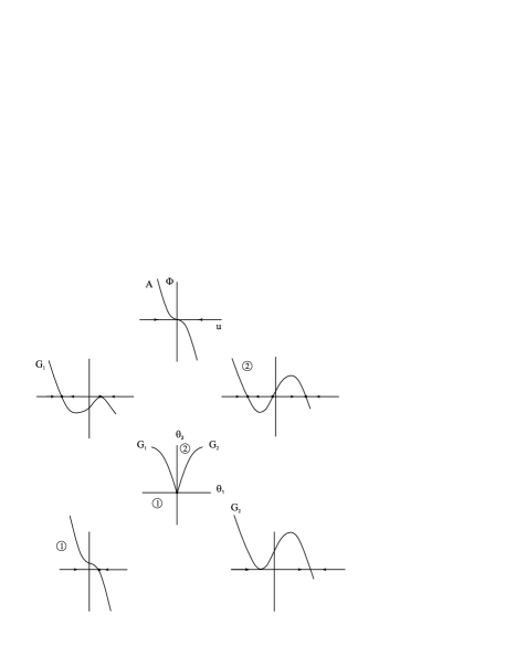
Figure 1.3: Bifurcation diagrams of the ”triple-equilibrium” bifurcation.

It should be noted that, for bifurcation values of the parameters, a projective mapping of the manifold $\psi\left(u,\theta_{1},\theta_{2}\right)=0$ onto the parameter space has fold-type singularities. The dynamic system in the neighborhood of the bifurcation exhibits hysteresis. Let us change the parameters in order to cross the semicubical parabola, while keeping watch on the stable equilibrium regime (Fig. 1.3). In the process of motion from left to right, the ”breakdown of equilibrium” of equilibrium occurs on the right branch $G_{2}$, whereas in the case of the reverse motion it occurs on the left branch $G_{1}$. This phenomenon is called ”a hysteresis loop”.

From formula (1.16), it is not difficult to obtain an explicit form of the bifurcation set in terms of the initial parameters $a_{1}$, $a_{2}$. Using (1.14) and (1.16), we derive the relation

$$8a_{1}a_{3}=3a_{2}^{2}.$$ (1.17)

Furthermore, if we take into account the expressions for $a_{1}$ and $a_{2}$ in terms of the demand and supply elasticities to price, using (1.8) and (1.11), we obtain the following expression for the bifurcation line:

$$8P_{E}^{3}a_{3}\eta=3Y_{E}\left(\eta^{\prime}P_{E}+\left(\eta_{D}+\eta_{S}-1\right)\eta\right)^{2}.$$ (1.18)

In the equality (1.18), the value of the excess-demand elasticity $\eta$ and its derivative with respect to the price $\eta^{\prime}$ are small quantities. Therefore, we can argue that the above-mentioned bifurcation can be observed in the initial dynamic system for very close values of the demand and supply elasticities, and of their derivatives, i.e.,

$$\eta_{D}\approx\eta_{S},\quad\eta_{D}^{\prime}\approx\eta_{S}^{\prime}.$$ (1.19)

Such a type of behavior cannot be explained by means of the methods of comparative statistics traditionally applied in economic analysis. Exactly the analysis of the dynamics of the system in the neighborhood of the state of equilibrium has shown that the behavior of the system is no longer characterized by a unique and smooth reaction to small shifts of the parameters. At the same time, there emerge a variety of states of equilibrium, including multiple and sudden jumps stipulated by the irreversibility of the flowing processes.

Analogously, one can carry out an investigation into the dynamics of the process of establishing the equilibrium value of production according to the concept of A. Marshall, described by the differential equation (1.3.) However, in contrast to the Walras model, in this case an analysis of the stability of the studied dynamic system involves such substantial economic characteristics as the values of elasticities of the prices of the demand and of the supply to the production volume.

It should be noted that the above results ask for more profound understanding of P. Samuelson’s principle of correspondence whose validity relies on the suggestion of predetermined stability of the economic system, with changeability bearing a smooth character.

1.2 A modified Walras-Marshall model

Up to now, we have considered the processes of changes of the market price and of the volume of commodity production as independent, and the mathematical models (1.8) and (1.11) have been studied separately. Therefore, in what follows, in order to study the dynamics of a model of a certain industrial object, we shall make an attempt to unify the equations of Walras and of Marshall into a single economic system, where the processes of production and of formation of the price are mutually related [13].

The issue of price formation in productive economic systems has always been and still remains relevant both for theoretical economic analysis and for the solution of concrete practical problems of the enterprise as well. In our view, it is important to synthesize two major factors of price formation. Thus, on the one hand, classical theory of market price formation argues that the market price corresponds to the equality of the demand and of the supply in the commodity market. On the other hand, according to the theory of the firm, it is known that, in the case of production balance, the price of the products manufactured by the enterprise corresponds to the marginal production costs. Thus, the first approach treats price formation from the point of view of the consumer, whereas the second one does it from the point of view of the producer. However, realities of the economic life witness that the processes of changes in the price and in the volume of production flow simultaneously and are interrelated. Therefore, it seems to be reasonable to consider the market mechanism of balancing the demand with the supply and the production process of accounting for the profit and costs simultaneously, within the framework of a unified dynamic system, according to the methodology presented in the work [5].

As the starting point, we consider a mathematical model describing the dynamics of the interaction between the prices and the volume of production (manufacturing):

$$\alpha\dot{P}=D\left(P\right)-Y,$$

$$\beta\dot{Y}=P-P_{S}\left(Y\right),$$ (1.20)

where $P$ is the price of the produced and sold product;

$Y$ is the volume of the product in natural terms (the market supply of the commodity);

$D\left(P\right)$ is the market demand for the product in natural terms;

$P_{S}\left(Y\right)$ is the supply price, equal to the marginal production costs, i.e., $P_{S}\left(Y\right)=C^{\prime}\left(Y\right)$;

$C^{\prime}\left(Y\right)$ are the production costs (expenses);

$\alpha$, $\beta$ are constant positive parameters describing characteristic times of transient processes.

The first equation of the system of the two ordinary differential equations (1.20) is the classical model of market price formation in the form of L. Walras (or P. Samuelson). They are based on the scheme of price formation searching for the balance between the demand and the supply: for $D\left(P\right)>Y$ the price rises, whereas for the opposite sign of the inequality it falls. The second equation of (1.20) describes the process of establishing the balance between the price and the marginal production costs with respect to the production (the value of production). Here, it is assumed that the balance is disturbed and it is necessary to regulate the volume of production: if $P>P_{S}\left(Y\right)$, the profit of the producer $P\cdot Y-C\left(Y\right)$ rises with an increasing the production volume, whereas in the opposite case one should decrease production activities.

The model is based on substantial simplifications. Firstly, the production is assumed to be single-product. Secondly, a local outlet without competition is considered, when the whole supply is formed by one producer. However, in spite of the above-mentioned assumptions, the model (1.20) admits complicated types of behavior, and their analysis will be the subject of further consideration.

A formal analysis of qualitative properties of system (1.20) should start with the consideration of singular solutions that characterize the states of equilibrium of the economic model.

By making the left-hand sides of (1.20) vanish, we obtain two constraint relations between equilibrium values of the price $P^{\ast}$ and of the volume $Y^{\ast}$:

$$D\left(P^{\ast}\right)=Y^{\ast},$$

$$P^{\ast}=P_{S}\left(Y^{\ast}\right).$$ (1.21)

Let us assume that the system of algebraic equations (1.20) has, at least, one positive solution $\left(P^{\ast},Y^{\ast}\right)$. concerning the volume of the demand $D\left(P\right)$, we point out that the dependence on the price is a substantially nonlinear function and there exists a Taylor expansion up to the third order in the neighborhood of the point $P^{\ast}$:

$$D\left(P\right)=d_{0}+d_{1}\left(P-P^{\ast}\right)+d_{2}\frac{\left(P-P^{\ast}\right)^{2}}{2}+d_{3}\frac{\left(P-P^{\ast}\right)^{3}}{6}+O\left(\left|P-P^{\ast}\right|^{4}\right),$$

where $d_{i}=\frac{dD^{i}\left(P^{\ast}\right)}{dP^{i}}$, $i=\overline{0,3}$.

The cost (expenses) function is represented by a quadratic function of the volume of production:

$$C\left(Y\right)=S_{1}\frac{Y^{2}}{2}+S_{0}Y+C_{0},$$

where $S_{1}$, $S_{0}$, $C_{0}$ are constant parameters.

Accordingly, the marginal costs (the supply price) are described by the formula

$$C^{\prime}\left(Y\right)=P_{S}\left(Y\right)=S_{1}Y+S_{0}.$$

Then, the system of equations (1.21) can be represented as follows:

$$S_{1}D\left(P^{\ast}\right)+S_{0}-P^{\ast}=0,$$

$$Y^{\ast}=\frac{P^{\ast}-S_{0}}{S_{1}}.$$ (1.22)

Having preliminarily changed the time scale, it is convenient to study the system (1.20) in terms of new variables that represent deviations from the equilibrium values $\tilde{P}=P-P^{\ast}$, $\tilde{Y}=Y-Y^{\ast}$. In this case, the system (1.20) reduces to the form

$$\overset{\cdot}{\tilde{P}}=d_{1}\tilde{P}+d_{2}\frac{\tilde{P}^{2}}{2}+d_{3}\frac{\tilde{P}^{3}}{6}-\tilde{Y},$$

$$\overset{\cdot}{\tilde{Y}}=\gamma\left(\tilde{P}-S_{1}\tilde{Y}\right),$$ (1.23)

where $\gamma=\frac{\alpha}{\beta}$.

As is obvious, equations (1.23) possess the trivial state of equilibrium $\tilde{P}=0$, $\tilde{Y}=0$.

To study the stability of the trivial state of equilibrium, we write down an explicit expression for the characteristic equation of the linear part of the system (1.23):

$$\lambda^{2}+\left(\gamma S_{1}-d_{1}\right)\lambda+\gamma\left(1-d_{1}S_{1}\right)=0.$$ (1.24)

The quadratic equation (1.24) has negative real parts under the conditions

$$\gamma S_{1}<d_{1},$$

$$S_{1}d_{1}<1.$$ (1.25)

The inequality (1.25) determines restrictions on the parameters of the initial system for stability in the linear approximation.

Let us consider in greater detail the situation in the vicinity of the boundary of the region of stability, taking into account the equality

$$\gamma C_{1}=d_{1}-\mu,$$ (1.26)

where $\mu$ is small, sign-alternating quantity. It is obvious that, in this case, the divergence of the vector field of the system (1.23) is equal to the small parameter $\mu$. Therefore, for $\mu<0$ the type of the singular point (the state of equilibrium) is a stable focus, whereas for $\mu>0$ it is an unstable focus. In other words, for $\mu=0$, in the neighborhood of the equilibrium state, there occurs the formation (annihilation) of a limit cycle as a result of the Hopf bifurcation.

Let us verify the validity of the conditions of Hopf’s theorem as applied to the system (1.23). The eigenvalues are determined (for $\mu=0$) by the equality

$$\lambda_{1,2}=\pm i\omega,$$ (1.27)

where $i^{2}=-1$, $\omega^{2}=\gamma-d_{1}^{2}$, i.e., they are purely imaginary. Upon the substitution of (1.26) in the quadratic equation (1.24) and subsequent differentiation with respect to the parameter $\mu$, we obtain for $\mu=0$:

$$\frac{d\lambda}{d\mu}=\lambda^{\prime}\left(0\right)=\frac{1}{2}-i\frac{d_{1}}{2\omega}.$$ (1.28)

From (1.28), it follows that the real part of the eigenvalue with respect to the parameter does not vanish, i.e., the eigenvalues in the complex plane cross the imaginary axis with a nonzero velocity. As a result, all the conditions of the Hopf bifurcation theorem are fulfilled.

Let us turn once again to (1.26) in order to give meaningful interpretation of this equality.

The above-mentioned condition can be fulfilled is the parameters $d_{1}$ and $S_{1}$ have the same sign. As in the following the value $S_{1}=C^{\prime\prime}\left(Y\right)$ will figure as the bifurcation parameter, its positivity characterizes concavity of the function of expenses $C\left(Y\right)$, whereas its negativity, accordingly, characterizes convexity. From an economic point of view, $S_{1}<0$ determines a positive effect of the volume of production ($C^{\prime\prime}\left(Y\right)<0$), whereas $S_{1}>0$ means that a rise in the costs outruns the output of the products ($C^{\prime\prime}\left(Y\right)>0$), i.e., the production is resource-consuming.

In order to determine essential parameters of the limit cycle that characterize its stability and the structure of periodic solutions, we reduce the system of differential equations (1.23) to the Poincaré normal form by means of a corresponding change of variables $\tilde{P}=x_{1}$, $\tilde{Y}=d_{1}x_{1}+\omega x_{2}$. As a result of the reduction, we obtain for $\mu=0$:

$$\dot{x}_{1}=-\omega x_{2}+\frac{d_{2}x_{1}^{2}}{2}+\frac{d_{3}x_{1}^{3}}{6},$$

$$\dot{x}_{2}=\omega x_{1}-\frac{d_{1}d_{2}}{\omega}\frac{x_{1}^{2}}{2}-\frac{d_{1}d_{3}}{\omega}\frac{x_{1}^{3}}{6}.$$ (1.29)

Using the explicit form of the coefficients of the nonlinear terms of the system (1.29), we derive an expression for the first Lyapunov quantity:

$$l_{1}\left(0\right)=\frac{d_{3}\left(\gamma-d_{1}^{2}\right)+d_{2}^{2}d_{1}}{16\left(\gamma-d_{1}^{2}\right)}.$$ (1.30)

For $l_{1}\left(0\right)<0$, a stable limit cycle takes place, and a corresponding regime of self-oscillations is called ”soft”. On the contrary, if $l_{1}\left(0\right)>0$, the limit cycle is unstable, the self-oscillations break down ”rigidly”, with a manifestation of irreversibility (hysteresis). The case $l_{1}\left(0\right)=0$ is the most complicated one in the sense of a variety of phase-plane structures of the system (1.29), because there appears a possibility of simultaneous coexistence of two limit cycles (with one being stable and the other one unstable) that subsequently merge into a single multiple limit cycle. This bifurcation has codimension two and will not be studied in detail in this Chapter.

The periodic solution of small amplitude $\varepsilon$ (up to a choice of the initial phase) is itself written down in the form [37]

$$P\left(t\right)=P^{\ast}+x_{1}\left(t\right),\quad Y\left(t\right)=Y^{\ast}+d_{1}x_{1}\left(t\right)+\omega x_{2}\left(t\right),$$

$$x_{1}\left(t\right)=\varepsilon\cos\left(\frac{2\pi t}{T}\right)$$

$$+\frac{\varepsilon^{2}d_{2}}{12\omega^{2}}\left[3d_{1}-d_{1}\cos\left(\frac{4\pi t}{T}\right)+2\omega\sin\left(\frac{4\pi t}{T}\right)\right]+O\left(\varepsilon^{3}\right),$$

$$x_{2}\left(t\right)=\varepsilon\sin\left(\frac{2\pi t}{T}\right)$$

$$+\frac{\varepsilon^{2}d_{2}}{12\omega^{2}}\left[3d_{1}-\omega\cos\left(\frac{4\pi t}{T}\right)-2d_{1}\omega\sin\left(\frac{4\pi t}{T}\right)\right]+O\left(\varepsilon^{3}\right).$$ (1.31)

Here, $\varepsilon^{2}=\frac{2\gamma\left(S_{1}-d_{1}\right)}{l_{1}\left(0\right)}$ is the amplitude; $T\left(\varepsilon\right)=\frac{2\pi}{\omega}\left(1+\tau_{2}\varepsilon^{2}+O\left(\varepsilon^{3}\right)\right)$, $\tau_{2}=\frac{d_{2}^{2}}{48\omega^{2}}\left(8+53\frac{d_{1}^{2}}{\omega^{2}}\right)$ is the period of the cycle depending, generally speaking, on the amplitude.

Thus, by the example of the system of two nonlinear differential equations (1.29), it is easy to establish that, in contrast to a linear system, periodic solutions are no longer harmonic, and the period and the amplitude of the oscillations are interrelated.

As an illustration of the obtained results, consider examples of economic-capacity cycles for different groups of commodities with regard to the dependence of the demand functions on the income, following the classification of the Swedish economist L. Tornquest [36].

Example 1. The demand function for essential commodities has a representation

$$E=\frac{q_{1}D}{D+C_{1}},$$

which reflects the fact that an increase in demand for these essential commodities gradually slows down with an increase in the income and has a has a limit $q_{1}>0$. The parameter $C_{1}$ is called the constant of half-saturation of the income.

Assuming that an equilibrium income is a function of the price,

$$E=PD\left(P\right),$$

we express the demand in the form $D=D\left(P\right)$. After corresponding transformations, we get

$$D\left(P\right)=\frac{q_{1}-C_{1}P}{P}.$$ (1.32)

With the help of (1.22) and (1.32), we write down the equation for an equilibrium price:

$$\left(P^{\ast}\right)^{2}-\left(S_{0}-S_{1}C_{1}\right)P^{\ast}-S_{1}q_{1}=0.$$ (1.33)

Differentiating (1.32) with respect to the price, we obtain the coefficients of the demand function:

$$d_{1}=-\frac{q_{1}}{\left(P^{\ast}\right)^{2}},\quad d_{1}=\frac{2q_{1}}{\left(P^{\ast}\right)^{3}},\quad d_{1}=-\frac{6q_{1}}{\left(P^{\ast}\right)^{4}}.$$ (1.34)

From (1.34), it follows that the quantities $d_{1}$, $d_{2}$ are negative numbers, and, therefore, by (1.30), the emerging limit cycle is stable. At the same time, the reason for the emergence of the cycle is the fact of positive influence of the effect of the scale of production of the given group of commodities, i.e., $S_{1}<0$.

Example 2. The demand-for-luxury-goods function is represented in the form

$$E=\frac{q_{1}D\left(D-b_{2}\right)}{D+C_{2}}.$$

By analogy with Example 1, we express the demand as a function of the price:

$$D\left(P\right)=\frac{C_{2}P+q_{2}b_{2}}{q_{2}-P},$$ (1.35)

where $q_{2}$, $b_{2}$, $C_{2}$ are positive parameters.

The equation for an equilibrium price has the form

$$\left(P^{\ast}\right)^{2}-\left(q_{2}+S_{0}-S_{1}C_{2}\right)P^{\ast}-q_{2}\left(S_{1}d+S_{0}\right)=0.$$ (1.36)

Assuming that (1.30) has at least one positive root $P^{\ast}$, we evaluate the coefficients of the powers of $P$:

$$d_{1}=\frac{q_{2}\left(b_{2}+C_{2}\right)}{\left(q_{2}-P^{\ast}\right)^{2}},\quad d_{2}=\frac{2q_{2}\left(b_{2}+C_{2}\right)}{\left(q_{2}-P^{\ast}\right)^{3}},\quad d_{3}=\frac{6q_{2}\left(b_{2}+C_{2}\right)}{\left(q_{2}-P^{\ast}\right)^{4}}.$$ (1.37)

In this case, the coefficients $d_{1}$ and $d_{2}$ are positive numbers, and the substitution of their values in (1.30) ensures the condition $l_{1}\left(0\right)>0$,  which is an indication of a catastrophic loss of stability of the limit cycle. As $d_{1}>0$, the emergence of a limit cycle requires the fulfillment of the condition $S_{1}>0$, which is possible only for resource-consuming production with an outrunning increase in the costs.

Let us consider one more version of the model (1.20), assuming, as a preliminary, that the supply price $P_{S}$ is a nonlinear function of the volume of production. For simplicity, we consider the quantities $P$ and $Y$ to be deviations from certain equilibrium values $P^{\ast}$ and $Y^{\ast}$.

Concerning the demand function $D\left(P\right)$ and the price, we put forward an assumption that they quadratically depend on their arguments, i.e.,

$$D\left(P\right)=d_{2}\frac{P^{2}}{2}-d_{1}P,$$

$$P_{S}\left(Y\right)=S_{2}\frac{Y^{2}}{2}-S_{1}Y.$$

Then, the system (1.20) can be represented in the form

$$\dot{P}=d_{2}\frac{P^{2}}{2}-d_{1}P-Y,$$

$$\dot{Y}=b^{2}\left(P+S_{1}Y-S_{2}\frac{Y^{2}}{2}\right),$$ (1.38)

where $b^{2}=\gamma$.

One can argue that a linear analysis of the stability of (1.38) completely corresponds to the previously obtained results for the system (1.23), including a verification of the validity of Hopf’s theorem, up to the substitution of $b^{2}$ for the parameter $\gamma$. Therefore, assuming the closeness of the bifurcation parameter $S_{1}$ to the quantity $\frac{d_{1}}{b^{2}}$, we transform (1.38) to the normal form of the given bifurcation with the help of the change of variables $x_{1}=P$, $x_{2}=\frac{Y-d_{1}P}{\omega}$ ($\omega^{2}=b^{2}-d_{1}^{2}$). After some transformations and the introduction of a new time scale $\tau=\omega t$, we obtain:

$$\dot{x}_{1}=-x_{2}+\frac{d_{2}x_{1}^{2}}{2},$$

$$\dot{x}_{2}=x_{1}+\frac{d_{1}\left(d_{2}-b^{2}d_{1}S_{2}\right)}{\omega^{2}}\frac{x_{1}^{2}}{2}+\frac{b^{2}d_{1}S_{2}}{\omega^{2}}x_{1}x_{2}-b^{2}S_{2}\frac{x_{2}^{2}}{2}.$$ (1.39)

Let us represent the system of two ordinary differential equations (1.39) in the form of a differential equation for the complex variable $Z=x_{1}+ix_{2}$, $\bar{Z}=x_{1}-ix_{2}$:

$$\dot{Z}=iZ+g_{20}\frac{Z^{2}}{2}+g_{11}Z\bar{Z}+g_{02}\frac{\bar{Z}^{2}}{2},$$ (1.40)

where $g_{11}=\frac{1}{4\omega}\left(d_{2}+\frac{i}{\omega}\left(d_{1}d_{2}-b^{4}S_{2}\right)\right)$;

$g_{20}=\frac{1}{4\omega}\left(d_{2}+2b^{2}d_{1}S_{2}+\frac{i}{\omega}\left(d_{1}d_{2}+b^{2}S_{2}\left(b^{2}-2d_{1}^{2}\right)\right)\right)$;

$g_{02}=\frac{1}{4\omega}\left(d_{2}-2b^{2}d_{1}S_{2}+\frac{i}{\omega}\left(d_{1}d_{2}+b^{2}S_{2}\left(b^{2}-2d_{1}^{2}\right)\right)\right)$.

Now, we possess all the necessary information for the evaluation of the first Lyapunov quantity

$$l_{1}=-\frac{1}{2}\mathop{\mathrm{I}m}g_{20}g_{11}.$$

Taking into account the explicit form of the coefficients of Eq. (1.40), we get:

$$l_{1}=\frac{d_{1}}{16\omega^{3}}\left(b^{6}S_{2}^{2}-d_{2}^{2}\right).$$ (1.41)

From (1.41), it is obvious that for $d_{2}^{2}>b^{6}S_{2}^{2}$ the limit cycle is stable, whereas for $d_{2}^{2}>b^{6}S_{2}^{2}$ the instability of the limit cycle takes place.

In Fig. 1.4, we present cyclic changes of the price and of the volume of the commodity of the considered state of equilibrium for the following values of the parameters of the system (1.38):

$$b=1;\quad d_{1}=0.5;\quad d_{2}=2;\quad S_{1}=0.5;\quad S_{2}=1.5.$$

The condition $d_{2}^{2}=\pm b^{3}S_{2}$ makes the expression for the first Lyapunov quantity vanish. This may mean that the initial system (1.38) possesses two limit cycles that can merge into one two-fold cycle by means of trajectory compaction. This situation is possible, if the second Lyapunov quantity, $l_{2}$, does not vanish. Setting for definiteness $S_{2}=\frac{d_{2}}{b^{3}}$, as a result of evaluation, we obtain $l_{2}=0$. Moreover, $l_{3}$, the next (third) Lyapunov quantity also vanishes under the given conditions. The fact that all the first three Lyapunov quantities vanish means that the state of equilibrium is a center, not a focus. In other words, the initial system (1.38), for

$$S_{1}=\frac{d_{1}}{b^{2}},\quad S_{2}=\frac{d_{2}}{b^{3}},$$ (1.42)

turns into a conservative one, with the conservation of the phase volume.

Let us write down the explicit form of (1.38), eliminating the parameters $S_{1}$,$S_{2}$ with the help of Eqs. (1.42):

$$\dot{P}=d_{2}\frac{P^{2}}{2}-d_{1}P-Y,$$

$$\dot{Y}=b^{2}P+d_{1}Y-\frac{d_{2}}{b}\frac{Y^{2}}{2}.$$ (1.43)

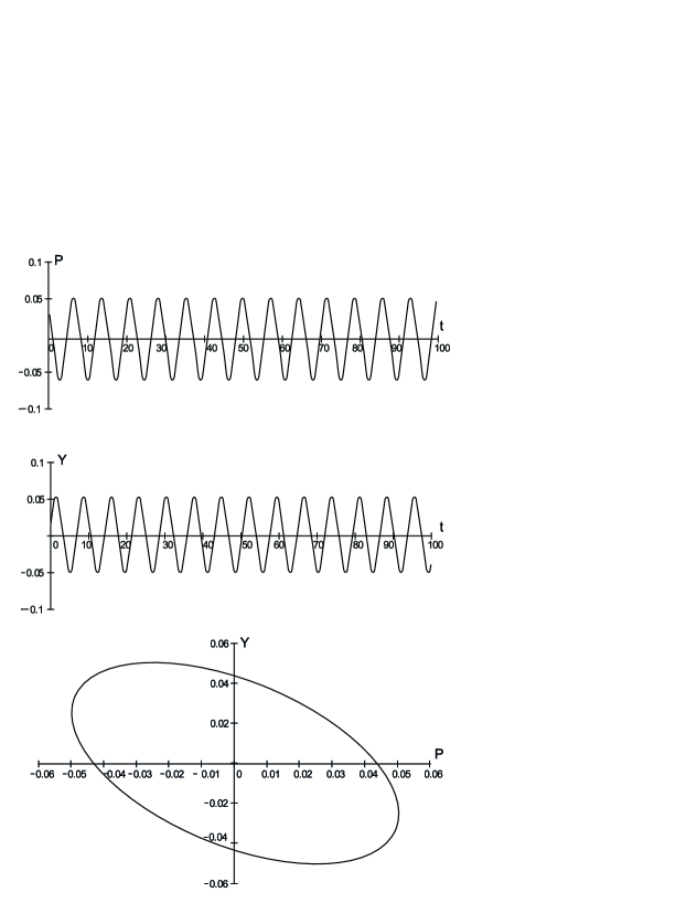
Figure 1.4: The limit cycle in the system (1.38).

It is important for us to find the first integral of the system (1.43). To this end, we transform the variables $P$ and $Y$ with the help of the linear substitution

$$Y_{1}=P-\frac{Y}{b},\quad Y_{2}=\frac{1}{\xi}\left(P+\frac{Y}{b}\right)+\frac{1}{2a},$$ (1.44)

where $\xi^{2}=\frac{b-d_{1}}{b+d_{1}}$, $a=\frac{d_{2}}{4\omega_{1}}$, $\omega^{2}=b^{2}-d_{1}^{2}$.

Then, equations (1.43) can be represented in the form

$$\dot{Y}_{1}=aY_{1}^{2}+a\xi^{2}Y_{2}^{2}-\left(\xi^{2}+1\right)Y_{2}+\frac{\xi^{2}+2}{4a},$$

$$\dot{Y}_{2}=2aY_{1}Y_{2}.$$ (1.45)

The system (1.45) can be reduced to a total differential equation:

$$\left(aY_{1}^{2}+a\xi^{2}Y_{2}^{2}-\left(\xi^{2}+1\right)Y_{2}+\frac{\xi^{2}+2}{4a}\right)dY_{2}=2aY_{1}Y_{2}dY_{1}.$$ (1.46)

By introducing the integrating factor $Y_{2}^{-2}$ into (1.45), we obtain the following equation:

$$\left(a\xi^{2}-\frac{\xi^{2}+1}{Y_{2}}+\frac{\xi^{2}+2}{4aY_{2}^{2}}\right)dY_{2}=2ad\left(\frac{Y_{1}^{2}}{Y_{2}}\right).$$ (1.47)

The integration of Eq. (1.45) yields

$$Y_{1}^{2}=\xi^{2}Y_{2}^{2}-\frac{\xi^{2}+1}{a}Y_{2}\ln\left|Y_{2}\right|+KY_{2}-\frac{\xi^{2}+2}{4a},$$ (1.48)

where $K$ is an arbitrary constant determined from the initial conditions.

Thus, expressions (1.44) and (1.48) determine a functional interrelation between the price and the volume of the commodity, which is a permanent balance between the income of the producer and his expenses at any moment of time.

Returning to the system (1.38), we should be reminded of the fact that the coefficients $d_{1}$, $d_{2}$ are the demand elasticity and its derivative with respect to the price, whereas $S_{1}$, $S_{2}$ are price demand elasticity and its derivative with respect to the volume of the commodity, i.e.,

$$d_{1}=\eta_{D},\quad d_{2}=\eta_{D}^{\prime},\quad S_{1}=\eta_{S},\quad S_{2}=\eta_{S}^{\prime}.$$

(It is understood that the elasticities and their derivatives are evaluated at the trivial state of equilibrium.)

Then, conditions (1.42) take a somewhat different form:

$$\eta_{D}=b^{2}\eta_{S},$$

$$\eta_{D}^{\prime}=b^{3}\eta_{S}^{\prime}.$$ (1.49)

The first expression in (1.49) implies a transition from a stable state of equilibrium to an unstable one with the formation (or annihilation) of a limit cycle, whereas the second expression in (1.49) determines the boundary between the types of stability of self-oscillation regimes.

Chapter 2 Periodic regimes in nonlinear models of the multiplier-accelerator

2.1 A multiplier-accelerator model with finite duration of an investment lag

In this Chapter, we consider an example of a certain kind of multiplier-accelerator models that illustrates at a phenomenological level different aspects of the problems of business cycles. As the starting point, we use the investment model of Goodwin [1] that possesses a nonlinear element built in the system of a multiplier-accelerator interaction. The dynamics of this model is characterized by the lag of two types: from the point of view of investment demand, there is a finite-duration lag of the action of the accelerator, whereas there is a continuously distributed lag on the part of supply.

As the main variable, the model involves profit or an output $Y=Y\left(t\right)$. An excess demand is formalized by the equation

$$D=C+I+G,$$ (2.1)

where $D$ is a cumulative demand comprising a consumer demand $C$, an investment demand $I$, and independent expenses $G$. All the above-mentioned terms are the actual costs. It is assumed that the consumption $C$ is directly proportional to the profit and the lag is absent, i.e., $C=cY$, where the quantity $0<c<1$ characterizes a marginal propensity to consume. We also assume that the actual investments outlay is carried out with a certain fixed lag of the duration of $\theta$ units of time after an investment decision $F\left(t\right)$ is made, i.e., $I\left(t\right)=F\left(t-\theta\right)$. Exactly here, the action of the accelerator manifests itself as a functional relation between the volume of investment decisions $F\left(t\right)$ and an instantaneous velocity of the change in the profit (output volume) $\frac{dY\left(t\right)}{dt}$. In the most general form, this relation can be represented as follows:

$$F\left(t\right)=\varphi\left(\frac{dY\left(t\right)}{dt}\right),$$

where $\varphi$ is a certain nonlinear function possessing the property of saturation.

In other words, for small changes in the profit, the classical linear accelerator comes into play, whereas for a further increase in the profit (output volume), the function $F$ reaches its upper bound $F_{\max}$ determined by the resource and capacity limits of the structure of the production.

When the volume of the production output substantially decreases, the quantity $F$ tends to its lower bound $F_{\min}$ that depends, generally speaking, on the amortization quota of the fixed capital. For the sake of convenience of further mathematical transformations, within the framework of the model under consideration, we restrict ourselves to a Taylor expansion of the function $\varphi\left(x\right)$ up to the third order:

$$\varphi\left(x\right)\approx\varphi_{1}x+\varphi_{2}\frac{x^{2}}{2}+\varphi_{3}\frac{x^{3}}{6},$$

where $\varphi_{i}$, $i=\overline{1,3}$, are corresponding derivatives of the function $\varphi\left(x\right)$.

Given that we have already described the main components of the cumulative demand function, we obtain the following equation:

$$D\left(t\right)=cY\left(t\right)+\varphi\left(\frac{dY\left(t\right)}{dt}\right)+G.$$ (2.2)

Concerning the independent expenses $G$, it should be noted that they can be considered fixed, i.e., $G=const$.

Consider next the situation on the part of supply. The main assumption is that value of the output volume $Y$ lags behind the value of the cumulative demand $D$. The lag is considered to be continuously distributed, and it can be represented by a linear first-order differential equation:

$$\varepsilon\frac{dY}{dt}=D-Y,$$ (2.3)

where $\varepsilon>0$ is a constant of the time lag characterizing the dynamics of adjustment between the demand and the supply.

A balance synthesis of the demand and the supply, by (2.2) and (2.3), yields a differential equation with a retarded argument:

$$\varepsilon\frac{dY\left(t\right)}{dt}-\varphi\left(\frac{dY\left(t-\theta\right)}{dt}\right)+\left(1-c\right)Y-G=0.$$ (2.4)

Equation (2.4) represents the general multiplier-accelerator model of Goodwin with nonlinear interactions.

With regard to the form of (2.4), it is nothing but a mixed differential-difference equation.

As is obvious, equation (2.4) has a singular solution $Y^{\ast}=\frac{G}{1-c}$ that represents an equilibrium level of profit (output volume) resulting from the action of the static multiplier. In what follows, it is reasonable to introduce the variable $y\left(t\right)=\frac{Y\left(t\right)-G}{1-c}$ that represents a deviation of the profit from its equilibrium value.

In terms of the new variable $y\left(t\right)$, equation (2.4) takes the form

$$\varepsilon s\frac{dy\left(t\right)}{dt}-\varphi\left(s\frac{dy\left(t-\theta\right)}{dt}\right)+s^{2}y\left(t\right)=0,$$ (2.5)

where $s=1-c$ is a marginal propensity to save.

The given model, represented by Eq. (2.5), determines the dynamics of profit (output volume) in terms of deviations from the above-mentioned equilibrium level $Y^{\ast}=\frac{G}{1-c}$.

For the sake of a further analysis of dynamic properties of the considered process of changes in profit, it is necessary to carry out a sequence of mathematical transformations and simplifications that will allow us to reduced the mixed first-order differential-difference equation to an ordinary differential equation of higher order [35].

Let us introduce new time $\tau=t-\theta$ instead of $t$. Then, equation (2.5) can be represented as

$$\varepsilon s\frac{dy\left(\tau+\theta\right)}{d\tau}-\varphi\left(s\frac{dy\left(\tau\right)}{d\tau}\right)+s^{2}y\left(\tau+\theta\right)=0.$$ (2.6)

Our next step consists in expanding the left-hand side of Eq. (2.6) into a power series in $\theta$, while retaining terms containing the first power of $\theta$. We obtain:

$$\varepsilon s\frac{dy\left(\tau\right)}{d\tau}+\varepsilon s\theta\frac{d^{2}y\left(\tau\right)}{d\tau^{2}}+s^{2}\left(y\left(\tau\right)+\theta\frac{dy\left(\tau\right)}{d\tau}\right)-\varphi\left(s\frac{dy\left(\tau\right)}{d\tau}\right)=0,$$

or

$$\varepsilon s\frac{d^{2}y}{d\tau^{2}}+\left(\varepsilon+\theta s\right)\frac{dy}{d\tau}-\frac{1}{s}\varphi\left(s\frac{dy}{d\tau}\right)+y=0.$$ (2.7)

In Eq. (2.7), we substitute the explicit form of the function $\varphi$ as a cubic polynomial. As a result of transformations, we obtain an ordinary second-order differential equation:

$$\frac{d^{2}y}{d\tau^{2}}+\left(\frac{\varepsilon+\theta s-\varphi_{1}}{\varepsilon\theta}\right)\frac{dy}{d\tau}+\frac{s}{\varepsilon\theta}y-\frac{s\varphi_{2}}{2\varepsilon\theta}\left(\frac{dy}{d\tau}\right)^{2}-\frac{s^{2}\varphi_{3}}{6\varepsilon\theta}\left(\frac{dy}{d\tau}\right)^{3}=0.$$ (2.8)

Making the change of variables $y=y_{1}$, $\frac{dy}{d\tau}=y_{2}$, we represent (2.8) in the form of a system of two differential equations:

$$\frac{dy_{1}}{d\tau}=y_{2},$$

$$\frac{dy_{2}}{d\tau}=-\frac{s}{\varepsilon\theta}y_{1}+\frac{\varphi_{1}-\varepsilon-\theta s}{\varepsilon\theta}y_{2}+\frac{s\varphi_{2}}{2\varepsilon\theta}y_{2}^{2}+\frac{s^{2}\varphi_{3}}{6\varepsilon\theta}y_{2}^{3}.$$ (2.9)

It is natural to begin the qualitative study of the dynamic system (2.9) from an investigation into the states of equilibrium. As is obvious, equations (2.9) possess only the trivial state of equilibrium $y_{1}^{\ast}=0$, $y_{2}^{\ast}=0$. To classify the type of this singular point, it is necessary to find characteristic numbers of the linear part of (2.9) determined by the quadratic equation

$$\lambda^{2}-\frac{\varphi_{1}-\varepsilon-\theta s}{\varepsilon\theta}\lambda+\frac{s}{\varepsilon\theta}=0.$$ (2.10)

From the explicit form of (2.10), one can infer that the singular point of the system (2.9) may be either a stable (unstable) node or a stable (unstable) focus. Of primary interest for us is the situation when a complex focus changes its stability, which may be accompanied by the formation of a limit cycle giving rise to a corresponding self-oscillation regime. In this case, we represent the solution of (2.10) in the form

$$\lambda_{1,2}=\frac{\mu}{2}\mp i\omega,$$ (2.11)

where $\omega^{2}=\frac{s}{\varepsilon\theta}$, $i^{2}=-1$, and $\mu=\frac{\varphi_{1}-\varepsilon-\theta s}{\varepsilon\theta}$ is a small quantity. In other words, for $\mu=0$, accordingly, the eigenvalues are purely imaginary: $\lambda_{1,2}=\mp i\omega$.

By differentiation expression (2.10) with respect to the parameter $\mu$, we obtain: $\lambda^{\prime}=\frac{d\lambda}{d\mu}=\frac{1}{2}$. This means that the eigenvalues $\lambda_{1,2}$ cross the imaginary axis with a nonzero velocity. Therefore, we can argue that the conditions of Hopf’s bifurcation theorem are fulfilled, and the system (2.9) allows for the formation of a limit cycle from the complex focus.

It would be in order here to draw attention to the reason for the occurrence of instability in the multiplier-accelerator model. As it seems, exactly the accelerator ”blows up” the damped oscillations induced by the multiplier and generates a structural self-sustained oscillation motion (self-oscillations). We have already seen that instability occurs in a given economic system when one of its parameters changes. It is most natural to consider as a variable parameter the coefficient of the linear accelerator $\varphi_{1}$ whose critical value $\varphi_{1}^{\ast}=\varepsilon+\theta s$ changes the direction of damping in the system (2.9). Thus, the coefficient $\varphi_{1}$ plays the role of a bifurcation parameter. The criterion of stability can now be written down in the form $\varphi_{1}<\varphi_{1}^{\ast}$. A linear analysis shows that when $\varphi_{1}$, while increasing, passes through the value $\varphi_{1}^{\ast}$, a loss of stability of the focus is caused by a pair of complex conjugate eigenvalues of the matrix of the coefficients of the linear part of the system (2.9).

The loss of stability at $\varphi_{1}=\varphi_{1}^{\ast}$ occurs under the conditions of Hopf’s theorem that states that, in addition to a stationary solution, there appear periodic solutions.

However, Hopf’s theorem itself does not provide information on whether these periodic solutions describe regimes that can be actually observed as steady ones. Periodic solutions may prove to be unstable and, accordingly, unobservable without the use of special procedures. Therefore, the next goal of our study of emerging periodic solutions in the system (2.9) is to derive explicit formulas describing their stability, amplitude, and period.

To achieve the above-mentioned goal, we shall use the techniques presented in [37]. For the sake of convenience of the application of the proposed methods, we shall retain original notation.

In order to reduce the system (2.9) to the normal Poincaré form, we make the change of variables $y_{1}=x_{1}$, $y_{2}=-\omega x_{2}$. As a result, for $\mu=0$, we obtain

$$\dot{x}_{1}=-\omega x_{2},$$

$$\dot{x}_{2}=\omega x_{1}-\frac{\omega^{3}\varphi_{2}}{2}x_{2}^{2}+\frac{\omega^{4}s\varphi_{3}}{6}x_{2}^{3}.$$ (2.12)

Let us represent the system of the two ordinary differential equations (2.12) in the form of a complex differential equation with respect to the variable $z=x_{1}+x_{2}$:

$$\dot{z}=i\omega z+g_{20}\frac{z^{2}}{2}+g_{11}z\bar{z}+g_{02}\frac{\bar{z}^{2}}{2}+g_{30}\frac{z^{3}}{6}+g_{21}\frac{z^{2}\bar{z}}{2}$$

$$+g_{12}\frac{z\bar{z}^{2}}{2}+g_{03}\frac{\bar{z}^{3}}{6},$$ (2.13)

where $\bar{z}$ is the complex conjugate of $z$, and the inverse change of variables yields $x_{1}=\mathop{\mathrm{R}e}z$, $x_{2}=\mathop{\mathrm{I}m}z$.

For further evaluation, we need only the coefficients $g_{20}$, $g_{11}$, $g_{02}$, and $g_{21}$. Their explicit forms are

$$g_{20}=-g_{11}=g_{02}=\frac{i\omega^{3}\varphi_{2}}{4},\quad g_{21}=\frac{\omega^{4}\varphi_{3}}{4}.$$ (2.14)

Given expressions (2.14), we obtain the following:

1) the value of the first Lyapunov quantity

$$\mathop{\mathrm{R}e}c_{1}\left(0\right)=\frac{s^{3}\varphi_{3}}{16\varepsilon^{2}\theta^{2}};$$ (2.15)

2) the amplitude of small oscillations

$$\rho=\sqrt{\frac{8\varepsilon\theta\left(\varphi_{1}-\varepsilon-\theta s\right)}{-s^{3}\varphi_{3}}};$$ (2.16)

3) an approximate value of the period of oscillations

$$T\approx\frac{2\pi}{\omega}\left(1+\frac{s^{2}\varphi_{2}^{2}}{24\varepsilon^{2}\theta^{2}}\rho^{2}\right).$$ (2.17)

The periodic solution itself, up to the choice of the initial phase, in terms of the original variable, is written down in the form

$$Y\left(\tau\right)=\frac{G}{s}+\rho\cos\left(\frac{2\pi\tau}{T}\right)+\frac{\rho^{2}s\varphi_{2}}{12\varepsilon\theta}\left(\cos\left(\frac{4\pi\tau}{T}\right)+3\right).$$ (2.18)

It is important for us to know the sign of the coefficients $\varphi_{3}$ that determines the sign of the first Lyapunov quantity in (2.15). For $\varphi_{3}>0$, $\mathop{\mathrm{R}e}c_{1}\left(0\right)>0$, and, accordingly, the limit cycle is unstable; that is, rigid excitation of self-oscillations takes place, accompanied by the phenomenon of hysteresis. However, the assumption of the positivity of $\varphi_{3}$ is unrealistic, because the condition of achieving the limit saturation $F_{\max}$ ($F_{\min}$) under an increase (decrease) in the velocity of changes of profit $Y$ will not be satisfied. Therefore, we should set $\varphi_{3}<0$ ($\mathop{\mathrm{R}e}c_{1}\left(0\right)<0$). In this case, a stable limit cycle is generated with a soft excitation regime of self-oscillations.

While analyzing the explicit form of the approximate solution for $Y\left(\tau\right)$ in expression (2.18), we should note the contribution of the coefficient $\varphi_{2}$. A nonzero value of $\varphi_{2}$ introduces certain asymmetry into the structure of the resulting oscillations. Obviously, they are nonharmonic even for small values of the amplitude. Besides, the coefficient $\varphi_{2}$ induces an increase in the period of oscillations with a growth in their amplitude.

An economic meaning of the asymmetry of the cycle consists in a difference between the duration of periods of expansion and that of periods of decline, which, on the whole, is a characteristic feature of nonlinear models of economic dynamics.

Somewhat earlier, we considered in detail the influence of the accelerator parameter $\varphi_{1}$ on the degeneracy of the linear part of the system (2.9) that directly induced a bifurcation of limit-cycle generation from an equilibrium state of the complex-focus type and the establishment of the regime of self-sustaining oscillations [12].

Summarizing, we want to emphasize that, in the present study of behavioral properties of the nonlinear multiplier-accelerator model of Goodwin, we have ascertained the mechanism of the occurrence of a cycle; we have determined the type of its stability, and we have given meaningful interpretation of the influence of all the parameters of the nonlinear accelerator on peculiarities of the self-oscillation regime.

2.2 A model of the multiplier-accelerator with a continuously distributed lag

In the previous Section, we have studied in detail an example of one nonlinear model of the multiplier-accelerator characterized by the occurrence of a stable limit cycle in the neighborhood of an equilibrium state. In that case, an essential element in the construction of the accelerator has been a finite-dimension lag in the functional relation between the measure of the volume of investment decisions and the instantaneous velocity of the change in profit (output volume). As basic assumptions in the synthesis of the initial model, we have employed nonlinear dependence of the accelerator on the derivative of profit, as well as linear dependence of the consumption function on the value of profit.

In the present consideration, the multiplier-accelerator model will be represented in a different form. First of all, we assume that the action of the accelerator is now expressed in terms of a continuously distributed lag [14].

According to R. Allen [1], if the investment function $I\left(t\right)$ represents the actually induced investment at the moment of time $t$, caused by changes in the output volume $Y\left(t\right)$, the lag is described by the differential equation

$$\frac{dI}{dt}=\beta\left(\varphi\left(\frac{dY}{dt}\right)-I\right),$$ (2.19)

where $\varphi$ is a nonlinear accelerator function, and the parameter $\beta>0$ characterizes the rate of changes in the investment function $I\left(t\right)$. Concerning $\varphi\left(\frac{dY}{dt}\right)$, it should be noted that its behavior for small changes in the profit is close to linear one, whereas with a further increase in $\frac{dY}{dt}$ the accelerator function grows slower and may even become non-monotonic. We shall assume that the mechanism of the action of the accelerator is satisfactorily described by the cubic parabola

$$\varphi\left(u\right)=\varphi_{1}u+\varphi_{2}\frac{u^{2}}{2}+\varphi_{3}\frac{u^{3}}{6},$$

where $\varphi_{i}$, $i=\overline{1,3}$, are corresponding derivatives of $\varphi\left(u\right)$.

The next step consists in the introduction of a lag into the model of the multiplier. In an analysis that follows, we shall also employ a continuous representation for the description of the action of the multiplier effect by means of a corresponding differential equation.

Let us assume that on the part of cumulative demand, a lag is absent. The planned consumption is given by $C=C\left(Y\right)$, and independent expenses are determined by the quantity $G.$

Then, the cumulative demand can be represented in the form of the equation

$$D=C\left(Y\right)+I+G.$$ (2.20)

Here, we give up the hypothesis that the consumption function is linear and assume that $C\left(Y\right)$ is a substantially nonlinear function of the output volume $Y$.

In the most general case, we restrict ourselves to representing $C\left(Y\right)$ in the form of a third-order polynomial, i.e.,

$$C\left(Y\right)=C_{1}Y+C_{2}\frac{Y^{2}}{2}+C_{3}\frac{Y^{3}}{6}.$$

The coefficients $C_{i}$, $i=\overline{1,3}$ have the same meaning as in the case of the accelerator function. Moreover, $C_{1}>0$, whereas $C_{1}$ and $C_{2}$ may have opposite signs.

The parameter of independent expenses $G$ is considered to be constant.

Consider the situation on the part of supply. Here, a response of the output volume $Y$ to the cumulative demand is considered to be non-instantaneous, inertial, i.e., there exists a continuously distributed lag in the form of a corresponding differential equation:

$$\frac{dY}{dt}=\alpha\left(D-Y\right),$$ (2.21)

where $\frac{1}{\alpha}$ is a time constant of the multiplier

Equations (2.19)-(2.21) completely determine the system of two nonlinear differential equations that describe an interaction between the multiplier and the accelerator. This system is represented as follows:

$$\frac{dY}{dt}=\alpha\left(C\left(Y\right)-Y+I+G\right),$$

$$\frac{dI}{dt}=\beta\left(\varphi\left(\frac{dY}{dt}\right)-I\right).$$ (2.22)

Given that $\varphi\left(0\right)=0$, the system (2.22) has singular solutions determined by the system of algebraic equations

$$C\left(Y\right)-Y+G=0,$$

$$I=0.$$ (2.23)

The first equation of (2.23), by the explicit form of $C\left(Y\right)$, may have up to three roots that represent the coordinates of an equilibrium state of the system (2.22).

We represent the system of two differential equations (2.22) in the form of a single second-order differential equation:

$$\frac{d^{2}Y}{dt^{2}}=\alpha\left(\left(C^{\prime}\left(Y\right)-1-\frac{\beta}{\alpha}\right)\frac{dY}{dt}+\beta\varphi\left(\frac{dY}{dt}\right)+\beta\left(C\left(Y\right)-Y+G\right)\right),$$ (2.24)

where $C^{\prime}\left(Y\right)=\frac{dC\left(Y\right)}{dY}$.

With the help of (2.24), we have succeeded in eliminating dependence on the variable $I\left(t\right)$. In what follows, we shall operate a vector field composed of the variables $Y\left(t\right)$ and $\frac{dY\left(t\right)}{dt}$. Introducing the coordinates $y_{1}=Y\left(t\right)$ and $y_{2}=\frac{dY\left(t\right)}{dt}$, it is reasonable to transform Eq. (2.24) into a system of two first-order differential equations:

$$\dot{y}_{1}=y_{2},$$

$$\dot{y}_{2}=\alpha\left(\left(C^{\prime}\left(y_{1}\right)-1-\frac{\beta}{\alpha}\right)y_{2}+\beta\left(\varphi\left(y_{2}\right)+C\left(y_{1}\right)-y_{1}+G\right)\right).$$ (2.25)

As is obvious, the system (2.25) possesses the same states of equilibrium as the system (2.24) does.

Let the coordinates of a single point be given as $\left(y_{1}^{\ast},y_{2}^{\ast}=0\right)$, where $y_{1}^{\ast}$ is the solution of the equation $C\left(y_{1}\right)-y_{1}+G=0$. In order to analyze behavioral properties of the system (2.25) in the neighborhood of the given state of equilibrium, we introduce new variables $u_{1}=y_{1}-y_{1}^{\ast}$ and $u_{2}=y_{2}$.

Given the explicit form of the nonlinear consumption function $C\left(Y\right)$, as a result of some transformations, we arrive at the system of differential equations

$$\dot{u}_{1}=u_{2},$$

$$\dot{u}_{2}=-\alpha\beta Su_{1}+\left(\alpha\beta\varphi_{1}-\beta-\alpha S\right)u_{2}+\alpha\beta\left(C_{3}y_{1}^{\ast}+C_{2}\right)\frac{u_{1}^{2}}{2}$$

$$+\alpha\left(C_{3}y_{1}^{\ast}+C_{2}\right)u_{1}u_{2}+\alpha\beta\varphi_{2}\frac{u_{2}^{2}}{2}+\alpha\beta C_{3}\frac{u_{1}^{3}}{6}$$

$$+\alpha C_{3}\frac{u_{1}^{2}u_{2}}{2}+\alpha\beta\varphi_{3}\frac{u_{2}^{3}}{6},$$ (2.26)

where $\ S=1-C_{1}-C_{2}y_{1}^{\ast}-C_{3}\frac{\left(y_{1}^{\ast}\right)^{2}}{2}$.

Let us consider a particular case of the system (2.26) under the conditions $\varphi_{2}=0$, $C_{3}y_{1}^{\ast}+C_{2}=0$. Under the above-mentioned restrictions, the quadratic terms in (2.26) vanish; that is, there is symmetry with respect to the change $u_{1}\leftrightarrow-u_{1}$, $u_{2}\leftrightarrow-u_{2}$. Furthermore, under the assumption that

$$G=-\frac{C_{2}\left(C_{2}^{2}+3C_{3}\left(1-C_{1}\right)\right)}{3C_{3}^{2}},$$

the equation for singular points $y_{1}$ is factorized as follows:

$$\left(C_{3}y_{1}+C_{2}\right)\left(\frac{y_{1}^{2}}{6}+\frac{C_{2}}{3C_{3}}y_{1}-\frac{C_{2}^{2}+3C_{3}\left(1-C_{1}\right)}{3C_{3}^{2}}\right)=0.$$ (2.27)

Accordingly, $y_{1}^{\ast}=-\frac{C_{2}}{C_{3}}$ is the coordinate of the state of equilibrium in whose neighborhood the behavior of the system (2.26) is being studied. To ensure the positivity of $y_{1}^{\ast}$, we assume that $C_{2}<0$, $C_{3}>0$, and the parameter$\ S=1-C_{1}+\frac{C_{2}^{2}}{2C_{3}}>0$.

After the above-mentioned simplifications, the system (2.26) takes the form

$$\dot{u}_{1}=u_{2},$$

$$\dot{u}_{2}=-\alpha\beta Su_{1}+\left(\alpha\beta\varphi_{1}-\beta-\alpha S\right)u_{2}+\alpha\beta C_{3}\frac{u_{1}^{3}}{6}$$

$$+\alpha C_{3}\frac{u_{1}^{2}u_{2}}{2}+\alpha\beta\varphi_{3}\frac{u_{2}^{3}}{6}.$$ (2.28)

We shall be concerned with qualitative properties of the system (2.28) in the neighborhood of the trivial state of equilibrium $u_{1}^{\ast}=0$, $u_{2}^{\ast}=0$. To determine the type of equilibrium, it is necessary to ascertain spectral properties of the linear part of (2.28) with the characteristic equation

$$\lambda^{2}-\mu_{1}\lambda+\alpha\beta S=0,$$ (2.29)

where $\mu_{1}=\alpha\beta\varphi_{1}-\alpha S-\beta$.

The explicit form of the quadratic equation (2.29) is analogous to that of the characteristic polynomial in [12]. Therefore, when analyzing the situation with the occurrence of a periodic regime in the system (2.29) resulting from the change of stability of the singular point of the type of a complex focus

$$\lambda_{1,2}=\frac{\mu_{1}}{2}\pm i\omega,\quad\omega^{2}=\alpha\beta S,$$

we can arrive at the conclusion that the reason for this effect is transition of the linear parameter of the accelerator through a certain critical value $\varphi_{1}^{C}=\frac{\alpha S+\beta}{\alpha\beta}$.

Note that the derivative of the eigenvalue $\lambda$ with respect to the parameter $\mu_{1}$ is nonzero:

$$\frac{d\lambda}{d\mu_{1}}=\frac{1}{2}\neq 0.$$

In this case, we may argue that the conditions of Hopf’s theorem are satisfied, and a limit cycle around the trivial state of equilibrium is generated in the system (2.28) from a complex focus.

The fact that a self-oscillation regime is present is rather remarkable in itself; however, it does not provide much information. Hopf’s bifurcation theorem does not give any answer to the question about the uniqueness of the limit cycle and the character of its stability.

To resolve the posed problems, we reduce (2.28) to the normal Poincaré form for $\mu_{1}=0$, using the change of variables $u_{1}=x_{1}$, $u_{2}=-\omega x_{2}$:

$$\dot{x}_{1}=-\omega x_{2},$$

$$\dot{x}_{2}=\omega x_{2}-\frac{\alpha\beta C_{3}}{\omega}\frac{x_{1}^{3}}{6}+\alpha C_{3}\frac{x_{1}^{2}x_{2}}{2}+\alpha\beta\varphi_{3}\omega^{2}\frac{x_{2}^{3}}{6}.$$ (2.30)

The system (2.30) can be reduced to the complex differential equation

$$\dot{Z}=i\omega Z+g_{30}\frac{Z^{3}}{6}+g_{21}\frac{Z^{2}\bar{Z}}{2}+g_{12}\frac{Z\bar{Z}^{2}}{2}+g_{03}\frac{\bar{Z}^{3}}{6},$$ (2.31)

where $Z=x_{1}+ix_{2}$, $\bar{Z}=x_{1}-ix_{2}$;

$$g_{30}=\frac{\alpha\left(3C_{3}-\beta\omega^{2}\varphi_{3}-\frac{i\beta C_{3}}{\omega}\right)}{8};\quad g_{21}=\frac{\alpha\left(C_{3}+\beta\omega^{2}\varphi_{3}-\frac{i\beta C_{3}}{\omega}\right)}{8};$$

$$g_{12}=\frac{\alpha\left(-C_{3}-\beta\omega^{2}\varphi_{3}-\frac{i\beta C_{3}}{\omega}\right)}{8};\quad g_{03}=\frac{\alpha\left(-3C_{3}+\beta\omega^{2}\varphi_{3}-\frac{i\beta C_{3}}{\omega}\right)}{8}.$$

Making use of the explicit expressions for the coefficients $g_{ij}$, it is not difficult to determine the first Lyapunov quantity:

$$l_{1}\left(0\right)=\mathop{\mathrm{R}e}\frac{g_{21}}{2}=\frac{\alpha\left(C_{3}+\beta\omega^{2}\varphi_{3}\right)}{16}.$$ (2.32)

As before [5], we assume that, as a result of the effect of investment saturation, $\varphi_{3}<0$, whereas the coefficient $C_{3}>0$. Therefore, a sign change in expression (2.32) is possible, which is a manifestation of different types of stability of the limit cycles. From (2.32), the stability of the limit cycle for $C_{3}+\beta\omega^{2}\varphi_{3}<0$ ($l_{1}\left(0\right)<0$) follows directly, whereas for the opposite sign of the inequalities an unstable self-oscillation regime with a catastrophic loss of stability takes place.

The case when the first Lyapunov quantity is small and alternates the sign, i.e.,

$$l_{1}=\mu_{2},$$ (2.33)

is of much greater interest.

As is well-known [6], the behavior of dynamic systems in the vicinity of the parameter values satisfying the equality $C_{3}+\beta\omega^{2}\varphi_{3}=0$, such that the first Lyapunov quantity $l_{1}$ vanishes, substantially depend on the sign of the second Lyapunov quantity $l_{2}$. Depending on the first and the second Lyapunov quantities, as well as on the sign of the real part of the roots of the characteristic equation $\mu_{1}$, in small neighborhood of the state of equilibrium on the phase plane, one or two limit cycles may exist with all possible combinations of stability and instability: namely, one stable or unstable limit cycle, or two limit cycles (a stable one inside an unstable one or vice versa).

The second Lyapunov quantity is determined by the expression

$$l_{2}=-\frac{1}{12\omega}\mathop{\mathrm{I}m}g_{30}g_{12}.$$ (2.34)

After substitution in (2.34) of the actual values of the parameters, we obtain:

$$l_{2}=\frac{\beta\alpha^{2}C_{3}}{6\omega^{2}}\left(C_{3}-\beta\omega^{2}\varphi_{3}\right),$$

or, by the validity of $C_{3}-\beta\omega^{2}\varphi_{3}=0$,

$$l_{2}=\frac{\beta\alpha^{2}C_{3}}{3\omega^{2}}.$$ (2.35)

As is obvious, the quantity $l_{2}$ does not vanish for any values of the parameters and is strictly positive, i.e., $l_{2}>0$.

If we make a conversion from the complex-valued variables to polar coordinates, we get two independent equations for the amplitude and the phase of the cycles:

$$\dot{\rho}=\rho\left(\mu_{1}+\mu_{2}\rho^{2}+l_{2}\rho^{4}\right),$$

$$\dot{\psi}=\omega.$$ (2.36)

The states of equilibrium for the first equation of (2.36) satisfy the biquadratic equation

$$\mu_{1}+\mu_{2}\rho^{2}+l_{2}\rho^{4}=0.$$ (2.37)

Equation (2.37) may have either none or one, or two positive solutions (cycles).

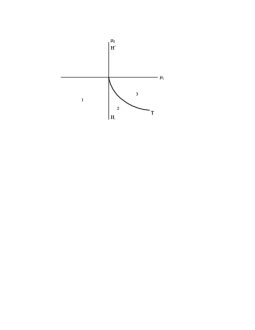
Figure 2.1: The bifurcation diagram.

In Fig. 2.1, we present the corresponding bifurcation diagram. The line $H=\left\{\left(\mu_{1},\mu_{2}\right):\mu_{1}=0\right\}$ relates to the usual Hopf’s bifurcation. The state of equilibrium is stable for $\mu_{1}<0$, and it is unstable for $\mu_{1}>0$. If we move along the line $\mu_{1}=0$ to the points where $\mu_{2}<0$, the complex second-order focus on the phase plane will generate an unstable (coarse) limit cycle, whereas the focus itself becomes non-coarse and stable. Should we enter, while crossing $H^{-}$, region 2, the stable complex focus generates a stable limit cycle. In region 2, both the cycle, the stable one and the unstable one, coexist simultaneously; the merge and disappear on the line $T=\left\{\left(\mu_{1},\mu_{2}\right):\mu_{2}^{2}=4l_{2}\mu_{1},\,\mu_{2}<0\right\}$.

The line $T$ characterizes the bifurcation of the double cycle. Further in region 3, limit cycles are absent.

In Fig. 2.2, the region of the coexistence of the two limit cycles is shown.

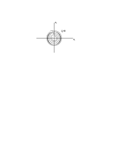
Figure 2.2: The stable and unstable limit cycles.

In conclusion of this investigation, we would like to point out the following: the presence of two limit cycles in the initial dynamic system of the multiplier-accelerator is stipulated not only by the nonlinearity of the accelerator function, but also by substantial nonlinearity of the consumption function, because exactly a relation between nonlinear coefficients of these functions ensures the bifurcation of the double cycle.

2.3 Cyclic regimes in a nonlinear model of the multiplier-accelerator with two degrees of freedom

Consider a model of the multiplier-accelerator with spatial inhomogeneity. Such a model reflects peculiarities of interregional trade in the presence of an import-export multiplier, which agrees with the already studied multiplier of local expenses, as well as with the general concept of Keynes and Samuelson [30, 31]. Let the quantity of an imported commodity depend on the local profit $Y$, which is now a function of time $t$ and of a generalized spatial coordinate $r$. Assuming, as the first approximation, that the action is local, we suppose that the commodity is imported from the nearest neighborhood of a considered point, whereas the exported product is produced under the influence of the same propensity to import in the neighborhood of this point. Then, the net trade surplus is determined by the product of a constant propensity to import and a profit margin in export-import operations. In other words, the above-said can be represented in the form of the following expression:

$$X-M=m\frac{\partial^{2}Y}{\partial r^{2}},$$

where $X$ is an export volume;

$M$ is an import volume;

$m$ is a constant propensity to import.

The spatial model of the multiplier-accelerator is represented in the form of a single second-order differential equation with a nonlinear investment function:

$$\frac{\partial^{2}Y}{\partial t^{2}}+SY-m\frac{\partial^{2}Y}{\partial r^{2}}=\left(\nu-1-S\right)\frac{\partial Y}{\partial t}-\frac{\nu}{3}\left(\frac{\partial Y}{\partial t}\right)^{3},$$ (2.38)

where $S$ is a marginal propensity to save;

$\nu$ is the coefficient of the accelerator.

In our consideration, we assume that all the parameters of the model, i.e., $S$, $\nu$, and $m$, are constant positive quantities that do not depend either on time or on the spatial coordinate.

The model described by Eq. (2.38) is a rather complicated mathematical object that exhibits a variety of forms of spatial-temporal organization. Therefore, in what follows we shall focus on dynamic processes, having preliminarily subdivided the space into two parts interrelated by the regional trade. This will allow us to study such phenomena as frequency matching and quasi-periodic motion. In other words, we may encounter a new form of the attractor, namely, an invariant torus.

The partial differential equation (2.38) is represented in the form of two coupled ordinary differential equations of the second order:

$$\ddot{Y}_{1}+\left(S_{1}+m_{1}\right)Y_{1}-m_{2}Y_{2}=\left(\nu_{1}-1-S_{1}\right)\dot{Y}_{1}-\frac{\nu_{1}}{3}\dot{Y}_{1}^{3},$$

$$\ddot{Y}_{2}+\left(S_{2}+m_{2}\right)Y_{2}-m_{1}Y_{1}=\left(\nu_{2}-1-S_{2}\right)\dot{Y}_{2}-\frac{\nu_{2}}{3}\dot{Y}_{2}^{3}.$$ (2.39)

Here, we have assumed that the parameters of the accelerator, the rates of accumulation and of import are different for each region of the subdivision.

Previously, for the model of the multiplier-accelerator in one region, we have found periodic regimes with the emergence of corresponding self-oscillations, and we have studied the character of their stability. As it seems, for the model with two regions, cyclic motion is also possible. Moreover, quasi-periodic motion with two matched frequencies is possible as well.

Let us represent the system (2.39) in the traditional form of a system of first-order differential equations. This new system is four-dimensional.

Let $x_{1}=Y_{1}$, $x_{2}=\dot{Y}_{1}$, $x_{3}=Y_{2}$, and $x_{4}=\dot{Y}_{2}$. As a result, the system (2.39) takes the form

$$\dot{x}_{1}=x_{2},$$

$$\dot{x}_{2}=-\left(S_{1}+m_{1}\right)x_{1}+\left(\nu_{1}-1-S_{1}\right)x_{2}+m_{2}x_{3}-\nu_{1}\frac{x_{2}^{3}}{3},$$

$$\dot{x}_{3}=x_{4},$$

$$\dot{x}_{4}=m_{1}x_{1}-\left(S_{2}+m_{2}\right)x_{3}+\left(\nu_{2}-1-S_{2}\right)x_{4}-\nu_{2}\frac{x_{4}^{3}}{3}.$$ (2.40)

Obviously, the system (2.40) has trivial equilibrium $x_{i}^{\ast}=0$, $i=\overline{1,4}$. The matrix of the linear part of (2.40), corresponding to this singular point, has the form

$$A=\left\{\begin{array}[]{cccc}0&1&0&0\\ -\left(S_{1}+m_{1}\right)&\nu_{1}-1-S_{1}&m_{2}&0\\ 0&0&0&1\\ m_{1}&0&-\left(S_{2}+m_{2}\right)&\nu_{2}-1-S_{2}\end{array}\right\}.$$ (2.41)

The matrix (2.41) has the characteristic polynomial

$$\left(\lambda^{2}-\left(\nu_{1}-1-S_{1}\right)\lambda+S_{1}+m_{1}\right)\left(\lambda^{2}\right.$$

$$\left.-\left(\nu_{2}-1-S_{2}\right)\lambda+S_{2}+m_{2}\right)-m_{1}m_{2}=0.$$ (2.42)

Equation (2.42) is a fourth-order equation; hence, it has four roots. Of primary interest for us is the situation when (2.42) has two pairs of complex conjugate roots with small parameters in their real parts, i.e.,

$$\lambda_{1,2}=\frac{\alpha_{1}}{2}\pm i\omega_{1},\quad\lambda_{3,4}=\frac{\alpha_{2}}{2}\pm i\omega_{2}.$$ (2.43)

Under the assumption that $\nu_{i}=1+S_{i}+\alpha_{i}$, $i=1,2$, there exist, for $\alpha_{i}=0$, critical values of the parameters of the accelerator $\nu_{i}^{c}=1+S_{i}$ that are responsible for a possible formation of limit cycles.

For $\alpha_{1}=\alpha_{2}=0$, equation (2.42) reduces to to the biquadratic equation

$$\lambda^{4}+\left(S_{1}+m_{1}+S_{2}+m_{2}\right)\lambda^{2}+\left(S_{1}+m_{1}\right)\left(S_{2}+m_{2}\right)-m_{1}m_{2}=0,$$

which, for $\lambda^{2}=-\omega^{2}$, yields an equation for the frequencies:

$$\omega^{4}-\left(S_{1}+m_{1}+S_{2}+m_{2}\right)\omega^{2}+\left(S_{1}+m_{1}\right)\left(S_{2}+m_{2}\right)-m_{1}m_{2}=0.$$ (2.44)

As the free term in (2.44) is positive, equation (2.44) has two positive roots that determine the squared frequencies:

$$\omega_{1,2}^{2}=\frac{\left(S_{1}+m_{1}+S_{2}+m_{2}\right)\pm\sqrt{D}}{2},$$

$$D=\left(S_{1}+m_{1}+S_{2}+m_{2}\right)^{2}-4\left(S_{1}+m_{1}\right)\left(S_{2}+m_{2}\right)-m_{1}m_{2}>0.$$

For definiteness, we assume that $\omega_{1}>\omega_{2}$. If we compare the values of the so-called eigenfrequencies $\bar{\omega}_{i}=\sqrt{S_{i}+m_{i}}$, $i=1,2$, it is not difficult to prove that $\omega_{1}>\bar{\omega}_{1}$, whereas $\omega_{2}<\bar{\omega}_{2}$. It means that the common frequency of the matched oscillations is either higher than the maximum natural frequency or lower than the minimum natural frequency. On the other hand, in the case of free oscillations, the matched system will never be able to oscillate with an intermediate, compared to natural frequencies, frequency. From an economic point of view, this fact means that a connection between two regions by means of trade relations either speeds up or slows down a cycle of business activity in both the regions.

For further consideration of the properties of the four-dimensional flux that possesses a state of equilibrium with two pairs of purely imaginary eigenvalues, it is necessary to construct the normal form for the system of ordinary differential equations (2.40). This can be done by means of a sequence of linear transformations of the initial variables as follows:

$$x_{1}=m_{2}\left(y_{1}+y_{3}\right),$$

$$x_{2}=-m_{2}\left(\omega_{1}y_{2}+\omega_{2}y_{4}\right),$$

$$x_{3}=\left(S_{1}+m_{1}-\omega_{1}^{2}\right)y_{1}+\left(S_{1}+m_{1}-\omega_{2}^{2}\right)y_{3},$$

$$x_{4}=-\omega_{1}\left(S_{1}+m_{1}-\omega_{1}^{2}\right)y_{2}-\omega_{2}\left(S_{1}+m_{1}-\omega_{2}^{2}\right)y_{4}.$$ (2.45)

The transformation (2.45) converts the system of four ordinary differential equations in real variables into a system of two complex differential equations that takes the following form in terms of the polar coordinates $Z_{j}=\rho_{j}e^{i\varphi_{j}}$:

$$\dot{\rho}_{1}=\alpha_{1}\rho_{1}+a_{11}\rho_{1}^{3}+a_{12}\rho_{1}\rho_{2}^{2},$$

$$\dot{\rho}_{2}=\alpha_{2}\rho_{2}+a_{21}\rho_{1}^{2}\rho_{2}+a_{22}\rho_{2}^{3},$$

$$\dot{\varphi}_{1}=\omega_{1}+O\left(\left|\rho\right|^{2}\right),$$

$$\dot{\varphi}_{2}=\omega_{2}+O\left(\left|\rho\right|^{2}\right).$$ (2.46)

Here, $\left|\rho\right|^{2}=\rho_{1}^{2}+\rho_{2}^{2}$; $\alpha_{1}$, $\alpha_{2}$ are small sign-alternating parameters; the coefficients $Z_{j}=\rho_{j}e^{i\varphi_{j}}$, $j=\overline{1,2}$, are functions of the initial parameters of the system.

We can learn a lot about the dynamics of the system (2.45) from the consideration of a plane vector field obtained by discarding the angular coordinates, following the methods proposed in [42].

In order to reduce the number of parameters, we scale the variables $\rho_{1}$ and $\rho_{2}$. Setting $\bar{\rho}_{1}=\rho_{1}\sqrt{\left|a_{11}\right|}$ and $\bar{\rho}_{2}=\rho_{2}\sqrt{\left|a_{22}\right|}\,$, dropping for notation convenience in what follows the bar over $\rho_{1}$ and $\rho_{2}$, and, if necessary, scaling the time variable, we obtain:

$$\dot{\rho}_{1}=\rho_{1}\left(\alpha_{1}+\rho_{1}^{2}+b\rho_{2}^{2}\right),$$

$$\dot{\rho}_{2}=\rho_{2}\left(\alpha_{2}+c\rho_{1}^{2}+d\rho_{2}^{2}\right),$$ (2.47)

$$d=\pm 1,\quad b=\frac{a_{12}}{\left|a_{22}\right|},\quad c=\frac{a_{21}}{\left|a_{11}\right|}.$$

The system (2.47) is characterized by twelve topologically different situations, presented in the following table:

Case	1	2	3	4	5	6	7	8	9	10	11	12
$d$	+	+	+	+	+	+	-	-	-	-	-	-
$b$	+	+	+	-	-	-	+	+	+	-	-	-
$c$	+	+	-	+	-	-	+	-	-	+	+	-
$d-bc$	+	-	+	+	+	-	-	+	-	+	-	-

This classification is based on an analysis of secondary ”pitchfork” bifurcations from nontrivial states of equilibrium of the plane vector field. Note that the singular point $\left(\rho_{1},\rho_{2}\right)=\left(0,0\right)$ is always a state of equilibrium; besides, up to three states of equilibrium may exist in the positive quadrant:

$$\left(\rho_{1},\rho_{2}\right)=\left(\sqrt{-\alpha_{1}},0\right),\quad\text{for }\alpha_{1}<0;$$

$$\left(\rho_{1},\rho_{2}\right)=\left(0,\sqrt{\frac{-\alpha_{2}}{d}}\right),\quad\text{for }\alpha_{2}d<0;$$ (2.48)

$$\left(\rho_{1},\rho_{2}\right)=\left(\sqrt{\frac{d\alpha_{2}-b\alpha_{1}}{Q}},\sqrt{\frac{c\alpha_{1}-\alpha_{2}}{Q}}\right),\quad\text{for }\frac{d\alpha_{2}-b\alpha_{1}}{Q},\frac{c\alpha_{1}-\alpha_{2}}{Q}<0,$$

where $Q=d-bc$, $d=\pm 1$.

In general, the behavior of the system remains comparatively simple until the occurrence of secondary Hopf bifurcations from the fixed point $\left(\rho_{1}^{\ast},\rho_{2}^{\ast}\right)=\left(\sqrt{\frac{d\alpha_{2}-b\alpha_{1}}{Q}},\sqrt{\frac{c\alpha_{1}-\alpha_{2}}{Q}}\right)$. In order to detect such bifurcations, we linearize the dynamic equations in a small neighborhood of this singular point. As a result, we obtain the following matrix:

$$T=\left(\begin{array}[]{cc}\alpha_{1}+3\left(\rho_{1}^{\ast}\right)^{2}+b\left(\rho_{2}^{\ast}\right)^{2}&2b\rho_{1}^{\ast}\rho_{2}^{\ast}\\ 2c\rho_{1}^{\ast}\rho_{2}^{\ast}&\alpha_{2}+c\left(\rho_{1}^{\ast}\right)^{2}+3d\left(\rho_{2}^{\ast}\right)^{2}\end{array}\right),$$

whose trace is

$$\mathop{\mathrm{t}r}T=\frac{2}{Q}\left(\alpha_{1}d\left(c-1\right)+\alpha_{2}\left(b-d\right)\right),$$

and the determinant is

$$\det T=\frac{4}{Q}\left(\left(b\alpha_{2}-d\alpha_{1}\right)\left(c\alpha_{1}-\alpha_{2}\right)\right).$$

Taking into account the conditions of the existence of the singular point (2.48), we infer that the secondary Hopf bifurcation may occur only on the straight line

$$\alpha_{2}=\frac{d\left(1-c\right)}{b-d}\alpha_{1},$$ (2.49)

and, at that, $Q>0$.

From this fact, it follows immediately that the secondary bifurcation does not occur in cases 2, 6, 7, 9, 11, 12. It is also possible to show that this bifurcation does not occur in cases 1, 3, 4, 5, because, for its realization, it is important that the angular coefficient of the straight line (2.49) should lie in between the angular coefficients of the straight lines that correspond to the ”pitchforks”, i.e.,

$$\alpha_{2}=c\alpha_{1},\quad\alpha_{2}=\frac{d}{b}\alpha_{1},$$ (2.50)

which is equivalent to

$$c<\frac{d\left(1-c\right)}{b-d}<\frac{d}{b}$$

in a corresponding sector of the plane $\left(\alpha_{1},\alpha_{2}\right)$.

As can be shown by means of simple evaluation, in each case, this requirement does not ensure the condition $Q>0$.

Consider case 8, in which a Hopf bifurcation may occur. Some bifurcation sets and phase portraits for this case are represented in Fig. 2.3.

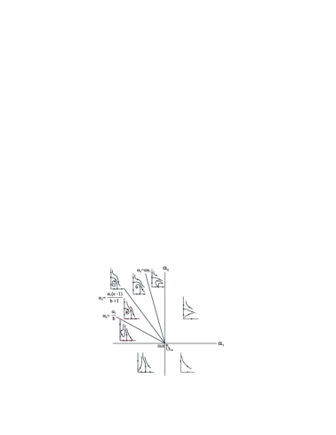
Figure 2.3: A partial bifurcation set of the secondary Hopf bifurcation.

On the Hopf-bifurcation line (2.49), the system

$$\dot{\rho}_{1}=\rho_{1}\left(\alpha_{1}+\rho_{1}^{2}+b\rho_{2}^{2}\right),$$

$$\dot{\rho}_{2}=\rho_{2}\left(\frac{c-1}{b+1}\alpha_{1}+c\rho_{1}^{2}-\rho_{2}^{2}\right)$$ (2.51)

is integrable, whereas the function

$$R\left(\rho_{1},\rho_{2}\right)=\rho_{1}^{\theta}\rho_{2}^{\beta}\left(\alpha_{1}+\rho_{1}^{2}+\gamma\rho_{2}^{2}\right),$$ (2.52)

with $\theta=\frac{2\left(1-c\right)}{Q}$, $\beta=\frac{2\left(1+b\right)}{Q}$, and $\gamma=\frac{1+b}{1-c}$, is constant along the solutions. In case 8, we have: $b>0>c$, $Q=-1-bc>0$, and $\alpha_{1}=-\alpha<0$; therefore, level lines of this function have the form shown in Fig. 2.4.

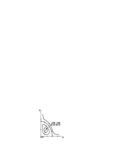
Figure 2.4: The level line $R\left(\rho_{1},\rho_{2}\right)$ for case 8.

As the system (2.51) is integrable, the secondary Hopf bifurcation is degenerate. Therefore, to study the topology of this bifurcation in full detail, it is necessary to consider in (2.49) terms containing higher powers of the initial variables.

Unfortunately, we do not possess necessary information, because nonlinearity in the accelerator model is restricted to cubic terms, whereas an exhaustive analysis requires terms of the fifth order. Nonetheless, it is possible to discuss some conclusions that can be drawn on the basis of the obtained results about the total four-dimensional flux of the system (2.46). It is necessary to bear in mind that here we have two rotations $\dot{\varphi}_{1}=\omega_{1}$ and $\dot{\varphi}_{2}=\omega_{2}$. Moreover, the ratio of the frequencies $\omega_{1}:\omega_{2}$ that should be restored for final conclusions. As is easy to see, the initial four-dimensional system (2.46) possesses four types of attractors corresponding to the fixed points of the plane system (2.47):

1) the trivial fixed point $\left(\rho_{1}=0,\rho_{2}=0\right)$;

2) a periodic orbit with the period $\approx\frac{2\pi}{\omega_{1}}\left(\rho_{1}=\rho_{1}^{\ast},\rho_{2}=0\right)$;

3) a periodic orbit with the period $\approx\frac{2\pi}{\omega_{2}}\left(\rho_{1}=0,\rho_{2}=\rho_{2}^{\ast}\right)$;

4) an invariant two-dimensional torus with the periods

$$\approx\frac{2\pi}{\omega_{1}},\quad\approx\frac{2\pi}{\omega_{2}}\left(\rho_{1}=0,\rho_{2}=\rho_{2}^{\ast}\right);$$

5) an invariant three-dimensional torus with the periods

$$\approx\frac{2\pi}{\omega_{1}},\quad\approx\frac{2\pi}{\omega_{2}},\quad O\left(\frac{1}{\alpha}\right).$$

The last (long) period on the tree-dimensional torus is associated with a secondary Hopf bifurcation in the plane system (2.47). Here, we can foresee the presence of subtle resonance effects and phenomena that remain outside the scope of our consideration. Thus, we expect to find a narrow ”wedge” around the line secondary Hopf bifurcation where chaotic dynamics, including transversal homoclinic orbits and ”horseshoes”, takes place. Consequently, we can argue that the multiplier-accelerator model of business cycles with a nonlinear investment function, extended to the case of interregional trade, and whose motion is induced by a linear multiplier of import, may initiate random motion.

This fact implies that processes of economic forecasting are problematic. As it seems, short-term forecasts are the most efficient ones, because exponential divergence of close trajectories does not occur over small periods of time.

Chapter 3 Self-organization in Keynesian models

As a science, macroeconomics was born owing to J. M. Keynes and, in the first place, to his outstanding work ”The General Theory of Employment, Interest and Money” where, for the first time, the problems of macroeconomics appeared as the main subject of the research. Keynes’s viewpoints, revolutionary at that time, had substantially formed as a result of an analysis of the reasons for the occurrence of the Great Depression. The global crisis of 1929-1933 prompted Keynes, as well as many other economists after him, to study seriously the economy as an integral system [27].

In this Chapter, we shall pay attention to some problems of economic dynamics, the models of which are based on the postulates of Keynes’s theory. As such, the following models will be successively considered:

1) the model of the growth of the gross domestic product;

2) the LS-LM Keynes model;

3) the Kaldor model.

3.1 The dynamics of GDP growth

In the construction of long-term programs of social-economic development and in macroeconomic modeling, the most important, in terms of criteria, factor is the volume of GDP per capita. Following the post-Keynesian tradition, consider, as the basis of the model of GDP growth, the main macroeconomic identity for the volume of the total income:

$$Y=C+I+G+N_{E},$$ (3.1)

where $Y$ is the GDP volume in value terms.

Let us analyze the terms of expression (3.1) from the point of view of their economic meaning.

1) $C=C\left(y\right)$ is the consumption volume that depends on GDP. We shall assume that $C\left(y\right)$ is a nonlinear function that can be represented by quadratic dependence:

$$C\left(y\right)=C_{0}+C_{1}y+C_{2}y^{2},$$

where $C_{0}$ is autonomous consumption; $C_{1}$ is the limit propensity to consume for small values of $y$; $C_{2}$ characterizes extremal properties of the consumption curve. If $C_{2}<0$, then $C\left(y\right)$ has a maximum, which agrees with Keynes’s postulate that the propensity to consume declines with an increase in income. For $C_{2}<0$, the function $C\left(y\right)$ has a minimum, according to the Modigliani-Duesenberry hypothesis of relative income [32].

2) $I=I\left(Y,\frac{dY}{dt}\right)$ is the investment function. We assume that investment react only to the rate of changes in GDP, i.e., it carries out the function of a simple accelerator:

$$I=\upsilon\frac{dY}{dt},$$

where $\upsilon$ is the marginal capital coefficient.

3) $G$ is the volume of government expenditure. In a simplified version, we assume that the quantity $G$ is independent of GDP and is constant in time.

4) $N_{E}$ is the volume of pure export characterizing the factor of external economic activities.

By analogy with $G$, we also assume that $\ N_{E}=\mathop{\mathrm{c}onst}$.

Taking into account all the above assumptions, we can represent the model (3.1) in the form of an ordinary differential equation:

$$\upsilon\frac{dY}{dt}=-R+\left(1-C_{1}\right)Y-C_{2}Y^{2},$$ (3.2)

where $R=C_{0}+G+N_{E}=\mathop{\mathrm{c}onst}$.

Singular solutions to Eq. (3.2) that correspond to states of static equilibrium can be found from the condition

$$\frac{dY}{dt}=0,$$

or

$$C_{2}Y^{2}-\left(1-C_{1}\right)Y+R=0.$$ (3.3)

The quadratic equation (3.3) has the following representation for the roots:

$$Y_{1,2}^{\ast}=\frac{1-C_{1}\pm\sqrt{A}}{2C_{2}},\quad A=-4C_{2}R+\left(1-C_{1}\right)^{2}.$$ (3.4)

If $C_{1}<1$, which is usually assumed, and $A>0$, then $Y_{1,2}^{\ast}$ are different positive numbers. In other words, equation (3.2) has two states of equilibrium, and the coefficients $C_{2}$ and$\ R$ have the same sign at that. In the case $A=0$, there exists a double state of equilibrium: $Y_{1,2}^{\ast}=\frac{1-C_{1}}{2C_{2}}$.

For $A<0$, equation (3.3) has no real solutions, i.e., equation (3.2) does not possess states of equilibrium. If the coefficients $C_{2}$ and$\ R$ have opposite signs, one of the roots is a positive number, whereas the other one is negative. As the negative solution has no economic meaning in this case, one speaks about a single state of equilibrium.

For the convenience of a further analysis of the properties of the differential equation (3.2), we introduce new variables $X=Y-\frac{1-C_{1}}{2C_{2}}$, $\tau=\frac{t}{\upsilon}$. As a result of the change of variables, equation (3.2) takes the form

$$\frac{dX}{d\tau}=\frac{A}{4C_{2}}-C_{2}X^{2}.$$ (3.5)

Expression (3.5) is a typical differential equation with separable variables. The integral curve that passes through the point $\tau=0$, $X\left(0\right)=X_{0}$ for $C_{2}>0$ is given by the following equations:

$$X\left(\tau\right)=\frac{X_{0}}{1+C_{2}X_{0}\tau},\quad\text{if }A=0;$$ (3.6)

$$X\left(\tau\right)=\frac{4X_{0}C_{2}\sqrt{A}+A\tanh\left(\sqrt{A}\tau\right)}{4C_{2}\sqrt{A}+4X_{0}C_{2}^{2}\tanh\left(\sqrt{A}\tau\right)},\quad\text{if }A>0;$$ (3.7)

$$X\left(\tau\right)=\frac{4X_{0}C_{2}\sqrt{-A}+A\tan\left(\sqrt{-A}\tau\right)}{4C_{2}\sqrt{-A}+4X_{0}C_{2}^{2}\tan\left(\sqrt{-A}\tau\right)},\quad\text{if }A<0.$$ (3.8)

It is not difficult to notice that, for different values of the quantity $A$, the solutions to the differential equation (3.5) differ substantially with regard to their properties, i.e., even for small variations of $A$ in the neighborhood of zero, a qualitative change in the scenario of the evolution of $X\left(\tau\right)$ takes place. Therefore, the development of the situation can be diagnosed by means of qualitative methods, without resort to complicated and expensive calculations. In qualitative forecasting, special attention should be paid to those factors that can change the dynamics of GDP growth either in negative or positive direction.

In other words, if the process under consideration is in a zone of stable development, the rest of qualitative information (such as the actual trajectory of development) becomes less important. As a rule, in macroeconomic modeling, mistakes and errors of approximation in the parameters of the model are possible; accounting for perturbations of exogenous character is also rather difficult. In this regard, it is reasonable to draw conclusions not about a single trajectory of development, but rather about a region of space of possible trajectories. The evaluation of such regions is the subject of qualitative theory of differential equations.

Let us normalize the variable $X\left(\tau\right)$ in such a way that will allow us to reduce the number of parameters in the differential equation (3.5) to a single one.

For $X\left(\tau\right)=-\frac{U\left(\tau\right)}{C_{2}}$, equation (3.5) takes the form

$$\frac{dU}{d\tau}=f\left(U,A\right),\quad f\left(U,A\right)=U^{2}-\frac{A}{4}.$$ (3.9)

Let $U^{\ast}=U^{\ast}\left(A\right)$ be a state of equilibrium of Eq. (3.9) for certain for certain fixed values of the parameter $A$, and let $\lambda\left(A\right)=f^{\prime}\left(U^{\ast},A\right)$.

For $\lambda<0$, the state of equilibrium $U^{\ast}$ is stable, whereas it is unstable for $\lambda>0$. For small variations of the parameter $A$, the behavior of the trajectory (3.9) in the neighborhood of the state of equilibrium with $\lambda\neq 0$ does not change qualitatively.

Thus, the inequality $\lambda\neq 0$ is the condition of non-degeneracy that singles out a coarse case.

In the neighborhood of the state of equilibrium, the coarse system is modeled by the linearized equation (3.9):

$$\frac{dU}{d\tau}=\lambda U,\quad\lambda\neq 0.$$ (3.10)

A different situation occurs when, for certain values of the parameter $A$, the eigenvalue $\lambda$ vanishes in the vicinity of the state of equilibrium:

$$\lambda\left(A\right)=f^{\prime}\left(U^{\ast},A\right)=0,$$

and the condition of non-degeneracy, $f"_{UU}\neq 0$, is fulfilled. In this case, $U^{\ast}$ is a double root of the equation $f\left(U^{\ast}\right)=0$.

A model equation for this bifurcation depends on a single parameter and has the form (3.9). Then, for $A>0$, the system (3.9) possesses two states of equilibrium: namely, a stable one and an unstable one. (The latter is the boundary of the attraction region of the stable state of equilibrium.) For $A=0$, they merge into a ”semi-stable” state of equilibrium and a non-coarse system appears. For $A<0$, the states of equilibrium disappear: see Fig. 3.1.

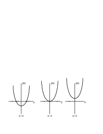
Figure 3.1: The bifurcation diagram for the case of ”double equilibrium”.

Let us monitor the stability of the state of equilibrium. Thus, when the parameter approaches the bifurcation value $A=0$, the attraction region shrinks on one side, and, after the disappearance of equilibrium, all the solutions leave the considered phase space. In economic applications, such a phenomenon is called ”a break-down of equilibrium”.

Note that, for the bifurcation value of the parameter $A=0$, the projective mapping $f\left(U,A\right)=0$ onto the parameter space has a ”fold”-type singularity. In other words, there occurs a loss of stability, i.e., a catastrophe of the ”fold” type.

An important quantitative parameter of the zone of stable development, in the model of economic development, is represented by the parameter $A$, which is a measure of the distance between the states of equilibrium $Y_{1}$ and $Y_{2}$ (or $X_{1}$ and $X_{2}$):

$$A=C_{2}^{2}\left(Y_{1}-Y_{2}\right)^{2}=C_{2}^{2}\left(X_{1}-X_{2}\right)^{2}.$$

In the case, when $A$ is sufficiently far from zero, one of the states of equilibrium is stable, whereas the second one is unstable. Such a situation is rather typical of, for example, the study of logistic economic growth. When $A$ tends to zero, the two states of equilibrium merge into a single one, and one can observe a state of dynamic uncertainty in the sense of the stability of economic growth trajectory, with a possible ”ejection” of the corresponding trajectory into the region of depressive dynamics. Returning to the basic macroeconomic equation (3.2), we can formulate the condition of stability: the derivative of the consumption function with respect to the GDP volume at the point of equilibrium should be larger that unity:

$$C_{Y}^{\prime}\left(Y^{\ast}\right)>1.$$ (3.11)

In this case, according to the Keynes absolute-income hypothesis, the consumption function is linear:

$$C\left(Y\right)=C_{0}+C_{1}Y.$$

Then, from (3.11), it follows that exponentially unstable growth is observed, because earlier we have assumed that the condition $C_{1}<1$ is fulfilled.

In other words, the model of economic growth with a linear consumption function can be stable only under the condition that a marginal propensity to consume is larger than unity. As is obvious, such a condition cannot be fulfilled in practice for an arbitrary GDP volume. This, in turn, induces a discussion about differences in the behavior of the consumption function in short-term and long-term periods.

The consumption function we have mentioned before and which rests on the relative-income hypothesis is devoid of such shortcomings.

Thus, the problem of studying the stability of economic growth, described by Eqs. (3.1) and (3.2), under the above-mentioned substantial simplifying assumption, has been reduced to structural properties of the consumption function. Quite naturally, there always exist certain parameters that, for some reason, do not fit into our formal analysis. This fact hampers the application of structural methods of macroeconomic forecasting, such as, e.g., simulative modeling. For this reason, in the present work, we employ the methodology of ascertaining, analyzing and forecasting economic processes and phenomena of self-organization by means of qualitative methods of the examination of dynamic models. By ascertaining substantially nonlinear processes of self-organization, we are able to single out the controlled factors as well as those factors that are beyond out influence [34].

As a result of our investigation, we have clearly demonstrated that the macroeconomic model of growth may have several states of static equilibrium. Accordingly, in dynamics, there exist evolutionary trajectories that correspond to the states of equilibrium of the system. In the case when the structure of the economy is coarse, small perturbations of the environment are unable to ”dislodge” it from its trajectory of growth. In the situation of a non-coarse system, even small jumps of the parameters (or a ”shock”) may cause a sudden transition to a different state of equilibrium, and the trajectories of development undergo qualitative changes. On the other hand, a merger of states of equilibrium is accompanied by a bifurcation with a catastrophic loss of stability. In this work, for a quadratic consumption function, we have studied effects in the vicinity of a double state of equilibrium, with the occurrence of a ”fold”-type catastrophe. Taking into account higher-order nonlinearity makes possible to observe a bifurcation of threefold degeneracy of the state of equilibrium, with an ”assembly”-type catastrophe, of fourfold degeneracy of the state of equilibrium, with an ”swallow-tail”-type catastrophe, etc.

A qualitative study of properties of the macroeconomic model should precede the elaboration of efficient methods of the management of the economic system on the basis of self-organization principles. The use of self-organization allows one to optimize shortages of the functioning of the economic system and to prevent the control parameters from entering a zone of undesirable bifurcations and catastrophes [22].

3.2 The LS-LM Keynes model

Consider the dynamic economic system proposed by J. M. Keynes in his work ”The General Theory of Employment, Interest and Money” [20]. This model represents the conditions of mutual balance in the goods and money market and is called, accordingly, the LS-LM model. In its simplest form, a business cycle is described by the system of ordinary differential equations

$$\tau_{Y}\frac{dY}{dt}=I\left(Y,R\right)-S\left(Y,R\right),$$

$$\tau_{R}\frac{dR}{dt}=L\left(Y,R\right)-M.$$ (3.12)

According to W. Zang [19], all the parameters and variables here are positive, and their meaning is the following: $Y=Y\left(t\right)$ is the volume of the national income; $R=R\left(t\right)$ is the interest rate; $I=I\left(Y,R\right)$ is the investment demand function that increases with respect to the volume of the national income, i.e., $\frac{\partial I}{\partial Y}=I_{Y}>0$, and decreases with respect to the interest rate, i.e., $\frac{\partial I}{\partial R}=-I_{R}<0$; $S=S\left(Y,R\right)$ is the savings function that increases with respect to both the variables, i.e., $\frac{\partial S}{\partial Y}=S_{Y}>0$, $\frac{\partial S}{\partial R}=S_{R}>0$; $L=L\left(Y,R\right)$ is the total demand for money that increases with respect to the income, i.e., $\frac{\partial L}{\partial Y}=L_{Y}>0$, and decreases with respect to the interest rate, i.e., $\frac{\partial L}{\partial R}=-L_{R}<0$; $M$ is the constant supply of money; $\tau_{Y}$ and $\tau_{R}$ are corresponding time constants.

The system (3.12) illustrates the action of a simple mechanism: an excess demand for investment, compared to the volume of savings, leads to an increase in the national income, and vice versa; in the case when the total demand for money resources is higher than the available supply, the interest rate increases.

Concerning the investment demand function, it should be noted that the values of $I\left(Y,R\right)$ stand in a direct relationship to the volume of the national income and in an inverse relationship to the interest rate. On the other hand, this means that an increase in the income or in the interest rate will stimulate the population to enhance the savings; and under the condition of growth in the output (income) volume, the demand for money $L\left(Y,R\right)$ increases.

For the system (3.12), we assume the existence of, as a minimum, one positive singular solution $Y_{0}$, $R_{0}$, which represents the state of static equilibrium of the LS-LM model. For algebraic evaluation of the combination of the values of the national income and of the interest rate, it is necessary to solve the following system of equations:

$$I\left(Y_{0},R_{0}\right)=S\left(Y_{0},R_{0}\right),$$

$$L\left(Y_{0},R_{0}\right)=M.$$ (3.13)

It is sufficient to confine the analysis of dynamic properties of the system (3.12) to a local domain of the two-dimensional space of the initial variables $Y\left(t\right)$ and $R\left(t\right)$ near the state of equilibrium $Y_{0}$, $R_{0}$.

To this end, we introduce new variables $\bar{Y}\left(t\right)=Y\left(t\right)-Y_{0}$ and $\bar{R}\left(t\right)=R\left(t\right)-R_{0}$, with the meaning of deviations from the equilibrium values of the income and of the interest rate, and expand the right-hand sides of the system (3.12) in a Taylor series at the point of equilibrium, retaining the first and the second powers of the corresponding variables. For convenience, we drop the bar over the variables and, without loss of generality, set $\tau_{R}=\tau_{Y}=1$, $F\left(Y,R\right)=I\left(Y,R\right)-S\left(Y,R\right)$.

As a result, the system (3.12) can be represented in the form

$$\frac{dY}{dt}=F_{Y}Y-F_{R}R+F_{YY}\frac{Y^{2}}{2}+F_{YR}YR+F_{RR}\frac{R^{2}}{2}+O\left(\left|Y\right|^{2},\left|R\right|^{2}\right)^{\frac{3}{2}},$$

$$\frac{dR}{dt}=L_{Y}Y-L_{R}R+L_{YY}\frac{Y^{2}}{2}+L_{YR}YR+L_{RR}\frac{R^{2}}{2}+O\left(\left|Y\right|^{2},\left|R\right|^{2}\right)^{\frac{3}{2}},$$ (3.14)

where the coefficients of the quadratic terms are the second-order derivatives with respect to the corresponding variables at the point of equilibrium $Y_{0}$, $R_{0}$, and $F_{Y}=I_{Y}-S_{R}>0$, $F_{R}=I_{Y}+S_{R}>0$.

The matrix of the linear part of (3.14) at the point of equilibrium has the following representation:

$$A=\left(\begin{array}[]{cc}F_{Y}&-F_{R}\\ L_{Y}&-L_{R}\end{array}\right),$$

with the characteristic polynomial

$$\lambda^{2}-\mathop{\mathrm{t}r}A\cdot\lambda+\det A=0,$$ (3.15)

where $\mathop{\mathrm{t}r}A=F_{Y}-L_{R}$ is the trace of the matrix $A$, and $\det A=F_{R}L_{Y}-F_{Y}L_{R}$ is the determinant of the matrix $A$.

In the case when $\mathop{\mathrm{t}r}A<0$ and $\det A>0$, we can argue that the system (3.14) is stable in the linear approximation. We shall consider in more detail the situation in a small neighborhood of the boundary of the region of linear stability $\mathop{\mathrm{t}r}A=\mu$, where $\mu$ is a small sign-alternating quantity. This means that the quantities $F_{Y}$ and $L_{R}$ are sufficiently close to each other, and when they are exactly equal to each other, the divergence of the vector field of the variables $Y\left(t\right)$, $R\left(t\right)$ passes through zero.

As $\det A>0$, we can set $\omega^{2}\left(\mu\right)=\det A=F_{R}L_{Y}-F_{Y}L_{R}$ and $F_{Y}=L_{R}+\mu$.

Equation (3.14) then takes the following form:

$$\lambda^{2}-\mu\lambda+\omega_{0}^{2}-\mu L_{R}=0,$$ (3.16)

$$\omega_{0}^{2}=F_{R}L_{Y}-L_{R}^{2}.$$

Differentiating (3.16) with respect to the parameter $\mu$, at $\mu=0$, we obtain:

$$\frac{d\lambda}{d\mu}=\frac{1}{2}-i\frac{L_{R}}{2\omega_{0}}.$$ (3.17)

From (3.16), it follows that the real part of the derivative of the eigenvalue does not vanish.

In other words, the eigenvalues cross the imaginary axis with a non-zero velocity.

Thus, the conditions of Hopf’s bifurcation theorem are fulfilled, and, in the system (3.14), when the stability of the complex-focus-type state of equilibrium changes, the formation (or annihilation) of a bifurcation of the limit cycle takes place, accompanied by the generation of a corresponding self-oscillation regime.

As a bifurcation parameter, we have chosen $F_{Y}=L_{R}$, which is equivalent to the condition

$$I_{Y}-S_{Y}-L_{R}=0.$$

To analyze this bifurcation, we construct, using the change of variables $Y=F_{R}x_{1}$, $R=L_{R}x_{1}+\omega_{0}x_{2}$, the normal form of the system (3.14) at $\mu=0$.

As a result of transformations with the change of the time scale $\tau=\omega t$, we obtain the system

$$\dot{x}_{1}=-x_{2}+a_{20}\frac{x_{1}^{2}}{2}+a_{11}x_{1}x_{2}+a_{02}\frac{x_{2}^{2}}{2},$$

$$\dot{x}_{2}=x_{1}+b_{20}\frac{x_{1}^{2}}{2}+b_{11}x_{1}x_{2}+b_{02}\frac{x_{2}^{2}}{2},$$ (3.18)

where

$$a_{20}=\frac{F_{R}^{2}F_{YY}+2F_{R}L_{R}F_{YR}+L_{R}^{2}F_{RR}}{\omega_{0}F_{R}};$$

$$a_{11}=F_{YR}+\frac{L_{R}F_{RR}}{F_{R}};\quad a_{02}=\frac{\omega_{0}F_{RR}}{F_{R}};$$

$$b_{20}=\frac{F_{R}^{2}\left(F_{R}L_{YY}-F_{YY}\right)+2F_{R}L_{R}\left(F_{R}L_{YR}-F_{YR}\right)+L_{R}^{2}\left(F_{R}L_{RR}-F_{RR}\right)}{\omega_{0}F_{R}};$$

$$b_{11}=\frac{F_{R}^{2}L_{YR}-F_{R}F_{YR}+L_{R}\left(F_{R}L_{RR}-F_{RR}\right)}{\omega_{0}F_{R}};\quad b_{02}=L_{RR}-\frac{F_{RR}}{F_{R}}.$$

The system of two ordinary differential equations (3.18) is the normal Poincaré form; it can be directly applied for the evaluation of the main characteristics of the forming limit cycles, such as the amplitude, the frequency, and the period of oscillations; it can also be applied for the determination of the stability of periodic solutions. The relevant formulas are given work by V. Zang [19]; it is shown therein that the limit cycle can be either stable or unstable, depending on the values of the typical parameters.

It would be in order here to emphasize that the above-mentioned work deals with the situation when the forming limit cycle is unique and has a quite definite type of stability. However, at the same time, the most important question in the studies of the Hopf bifurcation concerns the maximum number of limit cycles that can be generated from the state of equilibrium (the fixed point) under parametric excitation of the given system. This problem is completely resolved only for the quadratic case of polynomial systems by N. N. Bautin [6]: it is shown that the maximum number of limit cycles that can be generated in the quadratic system from a focus-type singular point is equal to three.

To determine maximum multiplicity of the limit cycle in the system of differential equations (3.18), it is necessary to evaluate the first three Lyapunov focus quantities.

Let us represent the system (3.18) in the form of a single complex differential equation in the variable $Z=x_{1}+ix_{2}$, for $\mu\neq 0$:

$$\dot{Z}=\left(i+\mu\right)z+g_{20}\frac{Z^{2}}{2}+g_{11}Z\bar{Z}+g_{20}\frac{\bar{Z}^{2}}{2},$$ (3.19)

where

$$g_{jk}=g_{jk}\left(a_{jk},b_{jk}\right),\quad j,k=\overline{0,2},\quad j+k=2.$$

The singular point turns from a focus into a center under the following conditions:

$$\text{1) }\mu=g_{11}=0;$$

$$\text{2) }\mu=g_{20}+\bar{g}_{11}=0;$$

$$\text{3) }\mu=\mathop{\mathrm{I}m}\left(g_{20}g_{11}\right)=\mathop{\mathrm{I}m}\left(\bar{g}_{11}^{3}g_{02}\right)=\mathop{\mathrm{I}m}\left(g_{20}^{3}g_{02}\right)=0;$$

$$\text{4) }\mu=g_{20}-4\bar{g}_{11}=\left|g_{02}\right|-2\left|g_{11}\right|=0.$$ (3.20)

Expressions (3.20) constitute the conditions for the existence of the first integral, or the Hamiltonian, of the system (3.18). In such a system, there exists an infinite set of periodic trajectories that continuously depend on the initial conditions. Quite naturally, isolated closed trajectories (limit cycles) cannot exist under the Hamiltonian conditions.

In the paper by H. Zoladek [48], the following formulas for the evaluation of the three Lyapunov quantities for Eq. (3.19) are given:

$$l_{1}=-\frac{1}{2}\mathop{\mathrm{I}m}\left(g_{20}g_{11}\right),$$

$$l_{2}=-\frac{1}{12}\mathop{\mathrm{I}m}\left(\left(g_{20}-4\bar{g}_{11}\right)\left(g_{20}+\bar{g}_{11}\right)\bar{g}_{11}g_{02}\right),$$ (3.21)

$$l_{3}=-\frac{5}{64}\mathop{\mathrm{I}m}\left(\left(4\left|g_{11}\right|^{2}-\left|g_{02}\right|^{2}\right)\left(g_{20}+\bar{g}_{11}\right)\bar{g}_{11}^{2}g_{02}\right).$$

Thus, using (3.21), it is not difficult to establish the cyclicity of the singular point:

1) no cycles are present if

$$\mu\neq 0;$$ (3.22)

2) a single cycle is present if

$$\mu=0,\quad\mathop{\mathrm{I}m}\left(g_{20}g_{11}\right)\neq 0;$$ (3.23)

3) two limit cycle coexist if

$$\mu=\mathop{\mathrm{I}m}\left(g_{20}g_{11}\right)=0,\quad g_{20}\neq 4\bar{g}_{11};$$ (3.24)

3) three limit cycles are observed if

$$\mu=g_{20}-4\bar{g}_{11}=0.$$ (3.25)

By virtue of the relation between (3.18) and (3.19), i.e.,

$$g_{20}=\frac{1}{4}\left(a_{20}-a_{02}+2b_{11}+i\left(b_{20}-b_{02}-2a_{11}\right)\right),$$

$$\bar{g}_{11}=\frac{1}{4}\left(a_{20}+a_{02}-i\left(b_{20}+b_{02}\right)\right),$$

we obtain a parametric restriction on the existence of three limit cycles.

According to the condition (3.25),

$$a_{20}-a_{02}+2b_{11}=4\left(a_{20}+a_{02}\right),$$

$$b_{20}-b_{02}-2a_{11}=-4\left(b_{20}+b_{02}\right),$$

or

$$2b_{11}=3a_{20}+5a_{02},$$

$$2a_{11}=5b_{20}+3b_{02}.$$ (3.26)

Relations (3.26) constitute algebraic conditions of the existence of three limit cycles in a system of the general form (3.18). They have been obtained by direct evaluation of the corresponding Lyapunov quantities for the six-parameter quadratic system without the use of any canonical models of the type of the system of Bautin, Andronova et al. [6], which employs a five-parameter form of the representation of considered models.

In the presence of parametric perturbations, we write down the following differential equation characterizing the dynamics of the amplitude of oscillations with three small parameters $\beta_{j}$, $j=\overline{1,3}$:

$$\dot{\rho}=\beta_{1}\rho+\beta_{2}\rho^{2}+\beta_{3}\rho^{3}+l_{3}\rho^{4}.$$ (3.27)

Here, $\beta_{1}=\mu$, $\beta_{2}=l_{1}$, $\beta_{3}=l_{2}$, and $l_{3}\neq 0$.

The bifurcation diagram of the system for the case $l_{3}<0$ is presented in Fig. 3.2 [4].

Figure 3.2: Relative disposition of bifurcation surfaces in the neighborhood of the bifurcation $l_{2}=0$.

The plane $N$ corresponds to bifurcation formation of a limit cycle from the fixed point $O$ (the state of equilibrium). On the half-plane $N_{-}$ the loss of stability of the focus is ”soft”, whereas it is ”rigid” on $N_{+}$. The curved surface $K$ corresponds to a non-local bifurcation of co-dimension one ”double cycle”. The part $K_{1}$ of this surface corresponds to a stable, from the outside, multiple cycle. The other part, $K_{2}$, corresponds to an unstable, from the outside, multiple cycle. On the surface $K$, there is a rib of return $C$, i.e., a common line for the above-mentioned parts of the surface of the multiple cycle. On the line $C$, there forms a non-local bifurcation of co-dimension two, i.e., a bifurcation of a merger of three cycles. The line of the intersection of the half-plane $N_{-}$ and the surface $K_{1}$ corresponds to a bifurcation of co-dimension ”one plus one” accompanied simultaneously by a change of the stability of the focus and a merger of a remote pair of cycles.

In Fig. 3.3, we present the bifurcation diagram in the neighborhood of $0$ (zero) for $l_{3}<0$.

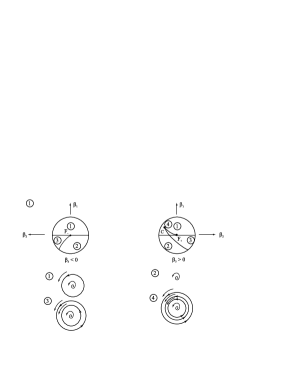
Figure 3.3: The bifurcation diagram for the bifurcation $l_{2}=0$ with $l_{3}<0$.

Returning to the description of the initial Keynes model (3.1), we want to emphasize that we have used a set of restrictions on the parameters of the linear part of the system (3.14) that has allowed us to satisfy the requirements of Hopf’s theorem on the existence of the limit cycle. At the same time, we have not stipulated any restrictive conditions on the coefficients of the quadratic terms, and, therefore, we may argue that, in the most general case, the maximum possible number of limit cycles in the neighborhood of the state of equilibrium $Y_{0}$, $R_{0}$ is equal to three.

Up to this point, we have studied the behavior of the system (3.14) on one boundary of the stability region determined by the trace of the matrices of dynamics. In what follows, we shall assume that both the trace and the determinant of this matrix are small sign-alternating quantities. Let $\det A=-\mu_{1}$ and $\mathop{\mathrm{t}r}A=\mu_{2}$.

In this case, the characteristic equation (3.15) takes the form

$$\lambda^{2}-\mu_{2}\lambda-\mu_{1}=0.$$ (3.28)

For $\mu_{1}=\mu_{2}=0$, the eigenvalues are multiple and equal to zero: $\lambda_{1,2}=0$. Such degeneracy in the linear part of (3.14) may lead to the formation of the Bogdanov-Takens bifurcation [7]; a study of this bifurcation is the subject of what follows.

As is obvious, in this case, one should choose two bifurcation parameter determined by the expressions for the trace and the determinant of the matrix $A$:

$$F_{Y}-L_{R}=\mu_{2},$$

$$F_{R}L_{Y}-F_{Y}L_{R}=-\mu_{1}.$$ (3.29)

Let the functions, found from condition (3.29), serve as the bifurcation parameters:

$$F_{Y}=L_{R}+\mu_{2},$$

$$F_{R}=\frac{L_{R}^{2}+L_{R}\mu_{2}-\mu_{1}}{L_{Y}}.$$ (3.30)

The next important stage is the construction of a corresponding normal form for the considered bifurcation of co-dimension two. Making the change of variables $Y=L_{R}y_{1}+y_{2}$, $R=L_{Y}y_{1}$, we obtain the following system:

$$\dot{y}_{1}=y_{2}+m_{20}y_{1}^{2}+m_{11}y_{1}y_{2}+m_{02}y_{2}^{2},$$

$$\dot{y}_{2}=\mu_{1}y_{1}+\mu_{2}y_{2}+n_{20}y_{1}^{2}+n_{11}y_{1}y_{2}+n_{02}y_{2}^{2},$$ (3.31)

where

$$m_{20}=\frac{L_{R}^{2}L_{YY}}{2L_{Y}}+L_{R}L_{YR}+\frac{L_{Y}L_{YR}}{2},$$

$$m_{11}=\frac{L_{R}L_{YR}}{L_{Y}}+L_{YR},\quad m_{02}=\frac{L_{Y}L_{YY}}{2},$$

$$n_{20}=\frac{1}{2}\left(L_{R}^{2}\left(F_{YY}-\frac{L_{R}}{L_{Y}}L_{YY}\right)+2L_{Y}L_{R}\left(F_{YR}-\frac{L_{R}}{L_{Y}}L_{YR}\right)\right.$$

$$\left.+L_{Y}^{2}\left(F_{RR}-\frac{L_{R}}{L_{Y}}L_{RR}\right)\right),$$

$$n_{11}=L_{R}\left(F_{YY}-\frac{L_{R}}{L_{Y}}L_{RR}\right)+L_{Y}\left(F_{YR}-\frac{L_{R}}{L_{Y}}L_{YR}\right),$$

$$n_{02}=\frac{L_{R}^{2}}{2}\left(F_{RR}-\frac{L_{R}}{L_{Y}}L_{RR}\right).$$

Carrying out a nonlinear reduction of the variables $y_{1}$ and $y_{2}$, i.e.,

$$y_{1}=u_{1}+\frac{m_{11}+n_{02}}{2}u_{1}^{2}+m_{02}u_{1}u_{2},$$

$$y_{2}=u_{2}-m_{02}u_{1}^{2}+n_{02}u_{1}u_{2},$$

and dropping terms of order higher than two, we arrive at the following system:

$$\dot{u}_{1}=u_{1},$$

$$\dot{u}_{2}=\mu_{1}u_{1}+\mu_{2}u_{2}+n_{20}u_{1}^{2}+\left(n_{11}+2m_{20}\right)u_{1}u_{2}.$$ (3.32)

By means of the substitution $w_{1}=u_{1}+\delta$, $w_{2}=u_{2}$, we eliminate from (3.32) the linear, in the variable $u_{2}$, term:

$$\dot{w}_{1}=w_{2},$$

$$\dot{w}_{2}=\theta_{1}+\theta_{2}w_{1}+n_{20}w_{1}^{2}+\left(n_{11}+2m_{20}\right)w_{1}w_{2}.$$ (3.33)

where

$$\theta_{1}=\frac{n_{20}}{\left(n_{11}+2m_{20}\right)^{2}}\mu_{2}^{2}-\frac{\mu_{1}\mu_{2}}{n_{11}+2m_{20}},$$

$$\theta_{2}=\mu_{1}-\frac{2n_{20}}{n_{11}+2m_{20}}\mu_{2}.$$

To complete the construction of the normal form of the system (3.31)-(3.33), we need yet another scaling of the variables, $\xi_{1}=\frac{w_{1}}{n_{20}K^{2}}$, $\xi_{1}=\frac{\mathop{\mathrm{s}ign}\left(K\right)}{n_{20}K^{2}}w_{2}$, and of time, $t=\left|K\right|\tau$, $K=\frac{n_{11}+2m_{20}}{n_{20}}\neq 0$:

$$\dot{\xi}_{1}=\xi_{2},$$

$$\dot{\xi}_{2}=\alpha_{1}+\alpha_{2}\xi_{1}+\xi_{1}^{2}+S\xi_{1}\xi_{2},$$ (3.34)

where

$$\alpha_{1}=\left(n_{11}+2m_{20}\right)K^{3}\theta_{1},\quad\alpha_{2}=K^{2}\theta_{2},\quad S=\mathop{\mathrm{s}ign}\left(K\right)=\pm 1.$$

Eliminating $\theta_{1}$ and $\theta_{2}$, we express the small parameters $a_{1}$, $\alpha_{2}$ in terms of $\mu_{1}$, $\mu_{2}$:

$$\alpha_{1}=K^{2}\mu_{2}^{2}-K^{3}\mu_{2}\mu_{1},$$

$$\alpha_{2}=K^{2}\mu_{1}-2K\mu_{2}.$$ (3.35)

The bifurcation diagram for the case $S=-1$ is represented in Fig. 3.4.

Figure 3.4: The diagram of the Bogdanov-Takens bifurcation in the system (3.34) for $S=-1$.

Our analysis of the system (3.34) we begin with the evaluations of the coordinates of the fixed point. As is obvious, since $\xi_{2}=0$, they are positioned on the horizontal axis in the phase plane and satisfy the quadratic equation

$$\alpha_{1}+\alpha_{2}\xi_{1}+\xi_{1}^{2}=0.$$ (3.36)

Equation (3.36) may have from zero to two roots. The discriminant parabola,

$$T=\left\{\left(\alpha_{1},\alpha_{2}\right):4\alpha_{1}-\alpha_{2}^{2}=0\right\},$$ (3.37)

is related to the ”fold” bifurcation. Along this line, the system (3.34) has equilibrium with the zero eigenvalue. If $\alpha_{2}\neq 0$, the ”fold” bifurcation is non-degenerate, and, on crossing the line $T$ from left to right, two states of equilibrium are formed.

Denoting the left and the right states of equilibrium by $E_{1}$ and $E_{2}$, respectively, we get:

$$E_{1,2}=\left(\xi_{1,2}^{0},0\right)=\left(\frac{1}{2}\left(-\alpha_{2}\pm\sqrt{\alpha_{2}^{2}-4\alpha_{1}}\right),0\right).$$

The point $\alpha=0$ separates the two branches, $T_{-}$ and $T_{+}$, of the ”fold”-bifurcation line for $\alpha_{2}<0$ and $\alpha_{2}>0$, respectively. Along the line $T_{-}$, a stable node $E_{1}$ coexists with a saddle point $E_{2}$, and, in the vicinity of $T_{+}$, an unstable node $E_{1}$ coexists with a saddle $E_{2}$.

The vertical line $\alpha_{1}=0$ is the line on which the state of equilibrium $E_{1}$ has a pair of eigenvalues of the zero sum: $\lambda_{1}+\lambda_{2}=0$. The lower part

$$H=\left\{\left(\alpha_{1},\alpha_{2}\right):\alpha_{1}=0,\,\alpha_{2}<0\right\}$$ (3.38)

is related to a non-degenerate Hopf bifurcation, whereas the upper half-line is a non-bifurcation line related to a neutral saddle. As a result of the Hopf bifurcation, a stable limit cycle is generated, i.e., the first Lyapunov quantity is negative.

The cycle exists in the neighborhood of $H$, for $\alpha_{1}<0$.

The state of equilibrium $E_{2}$ is still a saddle for all the values of the parameters to the left of the line $T$. Here, there are no other local bifurcations.

Let us pass around the point $\alpha_{1}=\alpha_{2}=0$ in circle of a small radius counterclockwise. In region 1, both states of equilibrium and cycles are absent. When passing from region 1 to region 2 through the part $T_{-}$ of the multiplicity line, two states of equilibrium are formed in the system (3.34): namely, a saddle $E_{2}$ and a stable node $E_{1}$. Further, the node turns into a focus that loses stability as a result of a Hopf bifurcation, which is accompanied by the formation of a stable limit cycle on the neutrality line of the focus $H$. This limit cycle disappears on the line $P=\left\{\left(\alpha_{1},\alpha_{2}\right):\alpha_{1}=-\frac{6}{25}\alpha_{2}^{2},\,\alpha_{2}<0\right\}$, being destroyed as a result of a global bifurcation on the loop of the separatrix of the saddle. (The period of motion along the cycle grows to infinity at that.) Finally, when passing from region 4 to region 1 through the part $T_{+}$ of the multiplicity line,  the unstable node merges with the saddle, and both of them disappear.

Using formulas (3.35), we write down the equations for the bifurcation lines in terms of the initial parameters $\mu_{1}$, $\mu_{2}$:

a) the line of the ”fold” bifurcation is given by

$$T=\left\{\left(\mu_{1},\mu_{2}\right):\mu_{1}=0,\,\mu_{2}\neq 0\right\};$$

b) the line of the Hopf bifurcation is given by

$$H=\left\{\left(\mu_{1},\mu_{2}\right):\mu_{2}\left(\mu_{2}-K\mu_{1}\right)=0,\,\mu_{2}>\frac{K}{2}\mu_{1}\right\};$$

c) the line of global bifurcation is given by

$$P=\left\{\left(\mu_{1},\mu_{2}\right):\left(7\mu_{2}-K\mu_{1}\right)\left(7\mu_{2}-6K\mu_{1}\right)=0,\,\mu_{2}>\frac{K}{2}\mu_{1}\right\}.$$

This point completes our study of the Bogdanov-Takens bifurcation of co-dimension two, as applied to the system (3.14). The case $S=+1$ can be studied using the substitution $t\rightarrow-t$, $\xi_{2}\rightarrow-\xi_{2}$. Here, a substantial difference lies in the instability of the limit cycle. Besides, it is important to note that the limit cycle in the vicinity of the point of the Bogdanov-Takens bifurcation has a frequency which is proportional to the square root of the small parameter. This means that a business cycle in the Keynes model may have a very large period, which rather difficult to detect in numerical simulations of the initial model.

3.3 Bifurcations in the nonlinear Kaldor model

The main assumption of this model, constructed in the Keynesian spirit, is that the investment and savings functions are substantially nonlinear functions of the income $Y$ and of the fixed assets rate $K$ [41]. As regards the investment function $I=I\left(Y,K\right)$, it is assumed that the limit propensity to invest $I_{Y}=\frac{\partial I}{\partial Y}$ is positive, although it is variable. This means that it takes the so-called ”normal” value for ”normal” values of the income rate $Y$. For values of income that are lower than a given ”normal” interval, the limit propensity to invest declines as a result of losses of income in the period of low activity rate compared to the ”normal” rate. It also decreases for values of $Y$ that are higher than the ”normal” interval because of a positive effect of the scale of expenditure and an increase in it. Thus, the investment function is an S-shaped curve. Besides, Kaldor assumes that a higher capital assets rate leads to a decrease in the marginal efficiency of the fixed assets; that is, $\frac{\partial I}{\partial K}=-I_{K}<0$ ($I_{K}>0$).

The savings function is also nonlinear: $S=S\left(Y,K\right)$. The limit propensity to save $S_{Y}=\frac{\partial S}{\partial Y}$ is positive and less than unity, although it varies. This assumption may be justified as follows: there exists a ”normal” rate of the propensity to save that corresponds to a ”normal” interval of changes in the income. Below this interval, the savings decrease towards consumption, whereas above this interval, they increase. In other words, the savings function is an upturned S-shaped curve.

Additionally, Kaldor assumes that $S_{K}=\frac{\partial S}{\partial K}$ is a positive quantity; that is, the savings function is shifted upwards with an increase in the capital rate. This assumption is questioned by a number of researchers [40, 44], because Kaldor himself did not provide any satisfactory justification for it. In our further consideration, we shall assume that $S_{K}$ may change sign.

In Fig. 3.5, we present qualitative dependencies of the investment and savings functions on the income rate, for a fixed value of the capital rate.

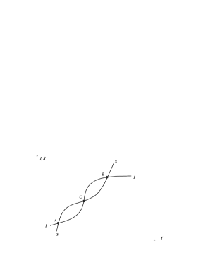
Figure 3.5: The structure of the states of equilibrium in the Kaldor model.

The dynamic Kaldor model is represented by the following equations:

$$\dot{Y}=\alpha\left[\left(I\left(Y,K\right)-S\left(Y,K\right)\right)\right],$$

$$\dot{K}=I_{0}\left(Y,K\right),$$ (3.39)

where $I_{0}\left(Y,K\right)$ is the realized investment, which, generally speaking, is different from the planned one $I\left(Y,K\right)$; the quantity $\alpha>0$ characterizes the rate of the change of the income in the time domain.

The functions $I\left(Y,K\right)$ and $S\left(Y,K\right)$ are symmetric with respect to the point of equilibrium. (Such an assumption is completely justified.) We also assume that the dependence of the above-mentioned functions on the variable $\ I$ is linear, and that the realized investment coincides with the planned one, i.e., $I_{0}=I$. It is then convenient to introduce new variables $\tilde{Y}=Y-Y_{0}$ and $\tilde{K}=K-K_{0}$ that constitute deviations of the initial investment and capital rates from their equilibrium values at the point $C$.

By symmetry, the investment and income functions are odd, and they can be represented in the following form:

$$I\left(\tilde{Y},\tilde{K}\right)=-I_{K}\tilde{K}+I_{Y}\tilde{Y}+I_{3}\tilde{Y}^{3}+O\left(\tilde{Y}^{5}\right),$$

$$S\left(\tilde{Y},\tilde{K}\right)=S_{K}\tilde{K}+S_{Y}\tilde{Y}+S_{3}\tilde{Y}^{3}+O\left(\tilde{Y}^{5}\right).$$ (3.40)

Here, $I_{3}$ and $S_{3}$ are the corresponding coefficients of the Taylor series expansion of the initial function, and, besides, the condition $I_{Y}>S_{Y}$ holds. Thus, the system (3.39) has the following explicit form:

$$\overset{\cdot}{\tilde{Y}}=\alpha\left(I_{Y}-S_{Y}\right)\tilde{Y}-\alpha\left(I_{K}-S_{K}\right)\tilde{K}+\alpha\left(I_{3}-S_{3}\right)\tilde{Y}^{3},$$

$$\overset{\cdot}{\tilde{K}}=I_{Y}\tilde{Y}-I_{K}\tilde{K}+I_{3}\tilde{Y}^{3}.$$ (3.41)

The system (3.41) has three states of equilibrium:

a) the trivial one, $\tilde{Y}_{0}=0$, $\tilde{K}_{0}=0$, which corresponds to the point $C$ in Fig. 3.5;

b) nontrivial ones, $\tilde{Y}_{1,2}=\mp\sqrt{-\frac{S_{Y}I_{K}+S_{K}I_{Y}}{S_{K}I_{3}+S_{3}I_{K}}}$, $\tilde{K}_{1,2}=\frac{S_{K}I_{Y}+S_{Y}I_{K}}{S_{3}I_{K}+S_{K}I_{3}}\tilde{Y}_{1,2}$, which corresponds to the points $A$ and $B$ in Fig. 3.5.

The points $A$, $B$ and $C$ represent possible variants of static equilibrium. In [41], it is argued that equilibrium at the point $C$ is unstable, whereas it is stable at the points $A$ and $B$. At the point $C$, the instability of equilibrium is due to the fact that, for $y_{A}<y<y_{C}$, savings exceed investments and a surplus appears in the goods market, which provokes a further decline in the production. In the case $y_{C}<y<y_{B}$, since the volume of investments exceeds that of savings, a deficiency of goods occurs, which stimulates a growth in the production.

As regards the stability of the points $A$ and $B$, we point out that a deviation from $A$ or $B$ to the right leads to a goods excess and to a decrease in their production, whereas a deviation to the left leads to a deficiency and to a growth in the production. The state of the economic system that corresponds to the point $A$ is characterized by a low volume of investments that is insufficient for a complete reimbursement of the worn-out capital. A decrease in the capital, after a certain time, will raise the entrepreneurs’ propensity to invest, and the demand for investments will grow, which will lead to an increase in the investment function $I\left(Y,K\right)$; equilibrium will be destroyed.

On the contrary, the point $B$ represents a state of equilibrium with high economic activities. As a result of an achieved optimal capital volume, the demand for investments starts to fall, the value of the function $I\left(Y,K\right)$ begins to decrease, and the economy leaves the state of equilibrium.

In the process of changes in market conditions, when the graphs of the savings and investment functions move towards each other, the points $A$ and $C$ may merge. In the opposite case, the points $B$ and $C$ may merge. It is important that these states of equilibrium, i.e., $A$, $B$ and $C$, become unstable.

In this regard, it is reasonable to study in detail the situation, when all the three states of equilibrium, $A$, $B$ and $C$, are sufficiently close to each other and may merge into a single point. Our further consideration will be devoted to a detailed analysis of properties of the dynamic system (3.41), taking into account the above-mentioned assumption.

Consider the behavior of the system (3.41) in the vicinity of the trivial state of equilibrium. The linear part of (3.41) has the characteristic polynomial

$$\lambda^{2}+\left(I_{K}-\alpha\left(I_{Y}-S_{Y}\right)\right)\lambda+\alpha\left(I_{Y}S_{K}+I_{K}S_{Y}\right)=0.$$ (3.42)

Let us assume that the coefficients in (3.42) are small quantities, i.e., $\mu_{1}=-\alpha\left(I_{Y}S_{K}+I_{K}S_{Y}\right)$ and $\mu_{2}=\alpha\left(I_{Y}-S_{Y}\right)-I_{K}$. In this case, the system (3.41) may have a Bogdanov-Takens bifurcation, i.e., a so-called ”double-zero” bifurcation [46]. As bifurcation parameters, we choose the following ones: $I_{K}=\alpha\left(I_{Y}-S_{Y}\right)-\mu_{2}$ and $S_{K}=-\frac{\alpha S_{Y}}{I_{Y}}\left(I_{Y}-S_{Y}\right)-\frac{\mu_{1}}{\alpha I_{Y}}+\mu_{2}$.

As $\mu_{1}$ and $\mu_{2}$ are small quantities, it is obvious that $S_{K}<0$. Making the change of variables $\tilde{Y}=\left[\alpha\left(I_{Y}-S_{Y}\right)-\mu_{2}\right]U_{1}+U_{2}$ and $\tilde{K}=I_{Y}U_{1}$, we reduce the system to the form of a nonlinear oscillator.

We have:

$$\dot{U}_{1}=U_{2}+a_{30}U_{1}^{3}+a_{21}U_{1}^{2}U_{2}+a_{12}U_{1}U_{2}^{2}+a_{03}U_{2}^{3},$$

$$\dot{U}_{2}=\mu_{1}U_{1}+\mu_{2}U_{2}+b_{30}U_{1}^{3}+b_{21}U_{1}^{2}U_{2}+b_{12}U_{1}U_{2}^{2}+b_{03}U_{2}^{3},$$ (3.43)

where

$$a_{30}=\frac{I_{3}}{I_{Y}}\left(\alpha\left(I_{Y}-S_{Y}\right)-\mu_{2}\right)^{3};\quad a_{21}=\frac{3I_{3}}{I_{Y}}\left(\alpha\left(I_{Y}-S_{Y}\right)-\mu_{2}\right)^{2};$$

$$a_{12}=\frac{3I_{3}}{I_{Y}}\left(\alpha\left(I_{Y}-S_{Y}\right)-\mu_{2}\right);\quad a_{30}=\frac{I_{3}}{I_{Y}};$$

$$b_{ij}=\left[\alpha\left(S_{Y}-\frac{S_{3}}{I_{3}}\right)+\mu_{2}\right]a_{ij};\quad i+j=3;\quad j=\overline{0,3}.$$

To construct the normal Poincaré form of the system of ordinary differential equations (3.43), we perform a nonlinear reduction of the variables of the state:

$$U_{1}=V_{1}+\left(\frac{a_{21}}{3}+\frac{b_{12}}{6}\right)V_{1}^{3}+\left(\frac{a_{12}+b_{03}}{2}\right)V_{1}^{2}V_{2}+a_{03}V_{1}V_{2}^{2},$$

$$U_{2}=V_{2}-a_{30}V_{1}^{3}+\frac{b_{12}}{2}V_{1}^{2}V_{2}+b_{03}V_{1}V_{2}^{2}.$$ (3.44)

As a result of transformations, taking into account expressions (3.44), we obtain the following representation of the system (3.43):

$$\dot{V}_{1}=V_{2},$$

$$\dot{V}_{2}=\mu_{1}V_{1}+\mu_{2}V_{2}+MV_{1}^{3}+NV_{1}^{2}V_{2},$$ (3.45)

where $M=b_{30}$, $N=b_{21}+3a_{30}$.

For $\mu_{1}=0$, $\mu_{2}=0$, we have: $N=3\alpha^{3}\left(I_{Y}-S_{Y}\right)^{2}\left(\frac{S_{Y}I_{3}}{I_{Y}}-S_{3}+I_{Y}-S_{Y}\right)$, $M=\alpha^{4}\left(I_{Y}-S_{Y}\right)^{3}\left(\frac{S_{Y}I_{3}}{I_{Y}}-S_{3}\right)$. It is reasonable to reduce the system (3.45), which is already a normal Poincaré form, to a still simpler form by means of the linear transformation

$$x_{1}=p\sqrt{\left|M\right|}V_{1},\quad x_{2}=p^{2}\sqrt{\left|M\right|}V_{2},\quad\tau=\frac{1}{p}t,$$

where

$$p=\left|\frac{N}{M}\right|=\frac{3}{\alpha}\left|\frac{1}{I_{Y}-S_{Y}}-\frac{1}{S_{3Y}-S_{Y}\frac{I_{3}}{I_{Y}}}\right|.$$

Finally, we get:

$$\dot{x}_{1}=x_{2},$$

$$\dot{x}_{2}=p^{2}\mu_{1}x_{1}+p\mu_{2}x_{2}+Sx_{1}^{3}-x_{1}^{2}x_{2},$$ (3.46)

where $S=\mathop{\mathrm{s}ign}\left(p\right)=\pm 1$.

As regards the system (3.46), it is not difficult to notice that it is invariant with respect to the substitution $x_{1}\rightarrow-x_{1}$ and $x_{2}\rightarrow-x_{2}$, and it always has trivial equilibrium $E_{0}=\left(0,0\right)$. The two other possible states of equilibrium have the coordinates $E_{1,2}=\left(\pm\sqrt{-S\mu_{1}},0\right)$; they exist for $\mu_{1}<0$, if $S=1$, and for $\mu_{1}>0$, if $S=-1$.

Important, for the system (3.46), is the fact that all the three states of equilibrium merge into the single trivial one for $\mu_{1}=0$.

Let $S=1$. The bifurcation diagram is presented in Fig. 3.6.

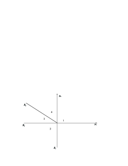
Figure 3.6: The bifurcation diagram for $S=+1$.

In region 1, there is the single trivial state of equilibrium $E_{0}$ that is a saddle point. On crossing the lower branch of the line $R_{1}=\left\{\left(\mu_{1},\mu_{2}\right):\mu_{1}=0\right\}$, a ”pitchfork” takes place, accompanied by the appearance of a pair of symmetric saddles $E_{1,2}$, until the trivial equilibrium $E_{0}$ becomes a stable node. This node turns into a focus in region 2 that, on crossing the half-line $R_{2}=\left\{\left(\mu_{1},\mu_{2}\right):\mu_{1}=0,\,\mu_{2}<0\right\}$, undergoes a Hopf bifurcation accompanied by the generation of a stable limit cycle.

On crossing the line $R_{3}=\left\{\left(\mu_{1},\mu_{2}\right):\mu_{2}=-\frac{p}{5}\mu_{1},\,\mu_{1}<0\right\}$, a global heteroclinic bifurcation, accompanied by the appearance of corresponding orbits that are related to the saddles $E_{1,2}$, takes place, and, in region 4, a heteroclinic cycle is formed. Further, all the three states of equilibrium coexist up to the crossing of the upper part of the straight line $R_{1}$, and a return to region 1 takes place.

Consider the case $S=-1$. The corresponding bifurcation diagram is depicted in Fig. 3.7.

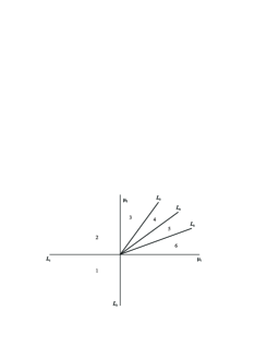
Figure 3.7: The bifurcation diagram for $S=-1$.

In region 1, there is the single trivial equilibrium $E_{0}$ that is a stable node; further, it goes over to a focus. On the half-line $L_{1}=\left\{\left(\mu_{1},\mu_{2}\right):\mu_{2}=0,\,\mu_{1}<0\right\}$, a Hopf bifurcation takes place, and a stable limit cycle is generated. Two unstable nodes separate from the trivial equilibrium on crossing the upper part of the line $L_{2}=\left\{\left(\mu_{1},\mu_{2}\right):\mu_{1}=0,\,\mu_{2}>0\right\}\,$, when passing from region 2 region 3, as a result of a ”pitchfork” bifurcation. In region 3, all the three states of equilibrium are localized inside a ”large” limit cycle. On the half-line $L_{3}=\left\{\left(\mu_{1},\mu_{2}\right):\mu_{2}=p\mu_{1},\,\mu_{1}>0\right\}$, the nontrivial focuses $E_{1,2}$ undergo a Hopf bifurcation. This bifurcation leads to the appearance of two ”small” unstable limit cycles around the nontrivial states of equilibrium. The points of equilibrium become stable. Thus, in region 4, there are three limit cycles: an external ”large” one and two internal ”small” ones. Along the line $L_{4}=\left\{\left(\mu_{1},\mu_{2}\right):\mu_{2}=\frac{4p}{5}\mu_{1},\,\mu_{1}>0\right\}$, the ”small” cycles form a symmetric figure that resembles the Bernoulli lemniscate, with the center at $E_{0}$, as a result of the occurrence of a global homoclinic bifurcation. Along the line $L_{4}$, the saddle $E_{0}$ has two homoclinic orbits. These orbits can be transformed from one into the other by means of symmetry transformations. On crossing the line $L_{4}$, when passing from region 4 to region 5, not only the ”small” cycles are destroyed, but also an external ”large” unstable cycle is generated. Then, in region 5, two ”large” cycles coexist: the external one is stable, while the internal one is unstable. These two cycles merge and disappear along the line $L_{5}=\left\{\left(\mu_{1},\mu_{2}\right):\mu_{2}=k_{0}p\mu_{1},\,\mu_{1}>0\right\}$, where $k_{0}=0.752\ldots$. This is a saddle-node bifurcation of the limit cycle. After the occurrence of this bifurcation, there are no limit cycles in the system. In region 6, all the three states of equilibrium are present: the trivial saddle $E_{0}$ and two stable nontrivial focuses (nodes) $E_{1,2}$. The nontrivial states of equilibrium merge with the trivial one on the lower part of the line $L_{2}=\left\{\left(\mu_{1},\mu_{2}\right):\mu_{1}=0,\,\mu_{2}>0\right\}$ as a result of a ”pitchfork” bifurcation, and we return to region 1.

Thus, the behavioral properties of the system (3.46) are determined by comparison between the quantities $I_{Y}-S_{Y}$ and $S_{3}-\frac{S_{Y}I_{3}}{I_{Y}}$. If the condition $I_{Y}-S_{Y}>S_{3}-\frac{S_{Y}I_{3}}{I_{Y}}$ is fulfilled, then $S=\mathop{\mathrm{s}ign}\left(p\right)=-1$. In the opposite case $I_{Y}-S_{Y}>S_{3}-\frac{S_{Y}I_{3}}{I_{Y}}$, we get: $S=+1$. Returning to the question of the choice of the sign of the quantity $S_{K}$, we note that states of equilibrium of the saddle type are possible in the initial dynamic system (3.41) only under the condition $S_{K}<-\frac{I_{K}S_{Y}}{I_{Y}}$, i.e., for $S_{K}<0$.

Thus, in this chapter, we have demonstrated dynamic behavior of the Kaldor model in its whole variety, in the case when three states of equilibrium degenerate into a single one. We have also followed the hierarchy of instabilities accompanied by a cascade of corresponding bifurcations [11].

Chapter 4 Dynamics of economic processes with a lag

In many economic models, when constructing balance relations, one has to take into account a lag responsible for various interactions. In Chapter 2, we have already considered the Goodwin model involving a lag of two types: on the part of the demand for investments there is a lag with fixed duration of the action of the accelerator, whereas on the part of the supply there is a continuously distributed lag. In this chapter, we shall demonstrate the application of methods of the theory of nonlinear oscillations in the class of differential equations with a lag and of integro-differential equations that may have a continuously distributed lag.

4.1 Instability of price dynamics in Fisher’s model

In modern economic literature, there is a sufficiently detailed qualitative description of the mechanism of the formation of domestic prices of the output based on an analysis of the dynamics of financial flows in export-import operations. At the same time, special attention is paid to such an important factor as an index of the trade balance whose surplus or deficit determines the direction of price change.

Before proceeding with the consideration of a formalized mathematical model based on classical Fisher’s macroeconomic equation, it is necessary to put forward a number of assumptions [41]:

1) a free-trade scheme, without any influence of governments and monopolistic structures, is considered;

2) the rate of the national income is considered to be sufficient, and the price rate is determined on the basis of qualitative theory of the currency of money;

3) in the course of the considered period, changes in the supply of money stock are stipulated exclusively by a surplus (or deficit) of the balance of trade;

4) since exchange rates are considered to be fixed, they can be set equal to unity, which is equivalent to complete unification of international operations;

5) transportation expenses, insurances and other costs are not taken into account either for commodity or financial flows.

In what follows, we use the following notation: $Q$ is money supply; $V$ is the rate of the currency of money; $Y$ is the national income rate (a constant); $P$ is the index of the domestic price; $P_{M}$ is the index of the export price (a constant); $M$ is the volume of import; $X$ is the volume of export.

The basic equation of Fisher’s model has the form

$$QV=PY.$$ (4.1)

The volume of export is a decreasing function of the domestic price:

$$X=X\left(P\right),\quad\frac{\partial X}{\partial P}<0.$$

On the contrary, the volume of import is an increasing function of the domestic price:

$$M=M\left(P\right),\quad\frac{\partial M}{\partial P}>0.$$

A relation of the form $P^{\ast}X\left(P^{\ast}\right)-P_{M}M\left(P^{\ast}\right)=0$ characterizes a condition of trade balance equilibrium, and it is assumed that this algebraic equation has positive solutions that determine equilibrium values of the domestic price $P^{\ast}$.

A disturbance of equilibrium is accompanied by changes in the money supply and is expressed by means of the following equation:

$$\frac{dQ}{dt}=PX\left(P\right)-P_{M}M\left(P\right).$$ (4.2)

From expression (4.1), it follows that a change in the money supply leads to a change in the domestic price $P=P\left(t\right)$. We assume that this change is not instantaneous, i.e., there is a time lag determined by a constant positive quantity $\tau$. In this case, equation (4.1) takes the form

$$\frac{dP\left(t\right)}{dt}=\frac{V}{Y}\frac{dQ\left(t-\tau\right)}{dt}.$$ (4.3)

From (4.2) and (4.3), we obtain a differential-difference equation that describes the dynamics of the domestic price:

$$\frac{dP\left(t\right)}{dt}=\frac{V}{Y}\left\{P\left(t-\tau\right)X\left[P\left(t-\tau\right)\right]-P_{M}M\left[P\left(t-\tau\right)\right]\right\}.$$ (4.4)

Let us assume that the export function $X\left(P\right)$ and import function $X\left(P\right)$ are inherently nonlinear and can be expanded in a Taylor series up to the third power in the neighborhood of the state of equilibrium $P^{\ast}$, i.e.,

$$X\left(P\right)=X_{0}+X_{1}\left(P-P^{\ast}\right)+X_{2}\left(P-P^{\ast}\right)^{2}+X_{3}\left(P-P^{\ast}\right)^{3}+O\left(P^{4}\right),$$

$$M\left(P\right)=M_{0}+M_{1}\left(P-P^{\ast}\right)+M_{2}\left(P-P^{\ast}\right)^{2}+M_{3}\left(P-P^{\ast}\right)^{3}+O\left(P^{4}\right),$$ (4.5)

where $X_{i}=\frac{\partial^{i}X\left(P^{\ast}\right)}{i!\partial P^{i}}$, $M_{i}=\frac{\partial^{i}M\left(P^{\ast}\right)}{i!\partial P^{i}}$, with $i=\overline{0,3}$, are corresponding derivatives of the functions $X\left(P\right)$ and $M\left(P\right)$ at the point of equilibrium $P^{\ast}$. We introduce a new variable $\bar{P}\left(t\right)=P\left(t\right)-P^{\ast}$ that has the meaning of a deviation of the domestic price from its equilibrium value. In this case, taking into account (4.5), equation (4.4) reduces to the following:

$$\frac{d\bar{P}}{d\bar{t}}=\frac{\tau V}{Y}\left[G_{1}\bar{P}\left(\bar{t}-1\right)+G_{2}\bar{P}^{2}\left(\bar{t}-1\right)+G_{3}\bar{P}^{3}\left(\bar{t}-1\right)+O\left(\bar{P}^{4}\right)\right],$$ (4.6)

where $\bar{t}=\tau t$, $G_{i}=X_{i-1}+P^{\ast}X_{i}-P_{M}M_{i}$, $i=\overline{1,3}$.

It is reasonable to begin an analysis of the process described by (4.6) with a study of the conditions of local stability, restricting ourselves only to the linear part, i.e.,

$$\frac{d\bar{P}}{d\bar{t}}=\frac{\tau V}{Y}G_{1}\bar{P}\left(\bar{t}-1\right).$$ (4.7)

The characteristic equation for (4.7) is given by

$$\lambda-\frac{\tau VG_{1}}{Y}e^{-\lambda}=0.$$ (4.8)

Using a well-known result of the theory of stability of differential-difference equations [43], as applied to (4.7), we obtain the necessary and sufficient conditions of linear stability:

$$0<-\frac{\tau VG_{1}}{Y}<\frac{\pi}{2}.$$ (4.9)

From the form of the left-hand part of the double inequality (4.9) it follows that the quantity $G_{1}$ is negative, whereas the right-hand part of (4.9) sets the upper bound for the absolute value of $G_{1}$.

Condition (4.9) has a rather transparent and meaningful interpretation. To demonstrate this interpretation, we perform a transformation of the initial parameters of the considered model (4.6).

Let

$$G_{1}=X_{0}\left[1-\eta_{X}-\eta_{M}\right],$$

where

$$\eta_{X}=\frac{P^{\ast}X_{1}}{X_{0}},\quad\eta_{M}=\frac{P^{\ast}M_{1}}{M_{0}},$$

under the condition $P^{\ast}X_{0}=P_{M}M_{0}$.

The quantities $\eta_{X}$ and $\eta_{M}$ are elasticities of the export and import functions with respect to the price $P$. As $X_{0}>0$, the condition $G_{1}<0$ is equivalent to $\eta_{X}+\eta_{M}>1$, which corresponds to the so-called Marshall-Lerner conditions [41]. At the same time, condition (4.9) reduces to

$$0<\eta_{X}+\eta_{M}<1+\frac{Y\pi}{2X_{0}V\tau}.$$ (4.10)

Thus, the economic interpretation of the conditions of local stability consists in the fact that the sum of the elasticities not only must be larger than unity, but it also must be smaller than an additional critical value. In other words, instability in the considered economic model may arise not only when the sum of the elasticities is sufficiently small, but also in the case when its value is much larger.

Let us study behavioral properties of the initial dynamic system (4.6) in a small neighborhood of the bounds of the inequality (4.10). First, we consider the situation when stability is lost at the lower bound. To this end, we introduce a small parameter $\nu_{1}=1-\eta_{X}-\eta_{M}$.

In this case, when the sign of $\nu_{1}$ changes, the eigenvalue of the linearized problem passes through zero, and a stationary value $P^{\ast}$ may either not exist or split into several stationary states. This means that a bifurcation of stationary solutions takes place.

The differential-difference equation (4.6) can be represented as follows:

$$\frac{d\bar{P}}{d\bar{t}}=A_{1}\bar{P}\left(\bar{t}-1\right)+A_{2}\bar{P}^{2}\left(\bar{t}-1\right)+A_{3}\bar{P}^{3}\left(\bar{t}-1\right),$$ (4.11)

where $A_{i}=\frac{\tau V}{Y}G_{i}$, $i=\overline{1,3}$.

One should bear in mind that the quantity $A_{1}$ is small, i.e., $G_{1}=X_{0}\nu_{1}$. Additionally, we assume that $A_{2}$ is also small if we introduce a small quantity $\nu_{2}=\frac{G_{2}}{X_{0}}$. Using the techniques of the central manifold method [46], one can prove that the differential-difference equation (4.11), under the condition that $A_{1}$, $A_{2}$ are small and the time lag is finite, is topologically equivalent to the differential equation

$$\frac{d\bar{P}}{d\bar{t}}=A_{1}\bar{P}\left(\bar{t}\right)+A_{2}\bar{P}^{2}\left(\bar{t}\right)+A_{3}\bar{P}^{3}\left(\bar{t}\right)$$ (4.12)

in the neighborhood of $\bar{P}=0$.

By means of the linear change of variables $\tilde{P}=\bar{P}+\frac{A_{2}}{3A_{3}}$, equation (4.12) is represented as follows:

$$\frac{d\tilde{P}}{d\bar{t}}=\alpha_{1}+\alpha_{2}\tilde{P}+\alpha_{3}\tilde{P}^{3},$$ (4.13)

where

$$\alpha_{1}=\frac{2A_{2}^{3}}{27A_{3}^{2}}-\frac{A_{1}A_{2}}{3A_{3}},\quad\alpha_{2}=A_{1}-\frac{A_{2}^{2}}{3A_{3}}.$$

The transformation $\tilde{P}\left(\bar{t}\right)=\left|\beta\right|W\left(\bar{t}\right)$ yields an explicit form of the normal Poincaré form for the differential equation (4.13):

$$\frac{dW}{d\bar{t}}=\beta_{1}+\beta_{2}W+SW^{3},$$ (4.14)

where

$$\beta=\frac{1}{\sqrt{A_{3}}},\quad\beta_{1}=\frac{\alpha_{1}}{\left|\beta\right|},\quad\beta_{2}=\alpha_{2},\quad S=\mathop{\mathrm{s}ign}\beta=\pm 1.$$

For definiteness, we set $S=-1$.

Equation (4.14) can have three states of equilibrium. A ”fold” bifurcation is determined by a curve $R$ on the plane $\beta_{1},\beta_{2}$, given by a projection of the line

$$\tilde{A}:\left\{\begin{array}[]{c}\beta_{1}+\beta_{2}V-V^{3}=0,\\ \beta_{2}-3V^{2}=0\end{array}\right.$$

to the parameter plane. By eliminating $V$ from these equations, we obtain the projection:

$$R=\left\{\left(\beta_{1},\beta_{2}\right):4\beta_{2}^{3}+27\beta_{1}^{2}=0\right\}.$$

The curve $R$ is called a semicubical parabola, and it has two branches $R_{1}$, $R_{2}$ that meet tangentially at the ”cusp-of-the-beak” point (a cusp bifurcation), for $\beta_{1}=\beta_{2}=0$. The corresponding bifurcation diagram is represented in Fig. 4.1.

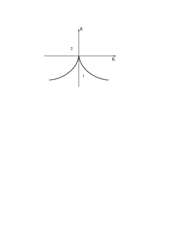
Figure 4.1: The diagram of the ”cusp-of-the-beak” bifurcation.

In region 1, in front of the boundary line, there are three states of equilibrium: two stable states and one unstable state. In region 2, behind the separation line, there is a single state of equilibrium which is stable. A non-degenerate ”fold” bifurcation takes place on crossing either $R_{1}$ or $R_{2}$ at any point of the parameter plane $\beta_{1},\beta_{2}$, except for the origin. If the curve is crossed on passing from region 1 to region 2, the right stable state of equilibrium merges with the unstable one, and both of them disappear. Analogously, the left stable state of equilibrium merges with the unstable one on the line $R_{2}$.

On approaching the ”cusp-of-the-beak” point, in front of the region1, all the three states of equilibrium merge into a single one as a triple root of the right-hand side of the initial equation (4.14). Of importance is also the fact that, in the course of the transition from a stable regime to an unstable one, the phenomenon of hysteresis is observed in (4.14), and a catastrophe occurs [46]. The case $S=1$ can be considered analogously.

Let us now clarify the situation when the sum of the elasticities $\eta_{X}+\eta_{M}$ is close to the right bound of the inequality (4.10). We introduce into consideration a small parameter $\mu=-\left(A_{1}+\frac{\pi}{2}\right)$. Then, the differential-difference equation (4.6) can be transformed into

$$\frac{d\bar{P}}{d\bar{t}}=-\left(\mu+\frac{\pi}{2}\right)\bar{P}\left(\bar{t}-1\right)+A_{2}\bar{P}^{2}\left(\bar{t}-1\right)+A_{3}\bar{P}^{3}\left(\bar{t}-1\right).$$ (4.15)

The characteristic equation for the linear part of (4.15) is given by

$$\lambda+\left(\mu+\frac{\pi}{2}\right)e^{-\lambda}=0.$$ (4.16)

We should find out when this equation has a pair of purely imaginary roots $\lambda=\pm i\omega$, $i^{2}=-1$, $\omega>0$.

If $\lambda=\pm i\omega$, then the conditions

$$\left(\mu+\frac{\pi}{2}\right)\cos\omega=0,\quad\omega-\left(\mu+\frac{\pi}{2}\right)\sin\omega=0$$

hold.

From this fact, it follows that, for $\mu=0$, equation (4.16) has a pair of purely imaginary roots for $\omega=\frac{\pi}{2}$. It is not difficult to show that (4.16) has no roots with positive real parts.

As $\lambda$ is analytic with respect to $\mu$, the differentiation of (4.16), at $\mu=0$, yields:

$$\frac{\partial\lambda}{\partial\mu}=\frac{\frac{\pi}{2}+i}{\frac{\pi^{2}}{4}+1}.$$

Thus, all the conditions of Hopf’s theorem on the existence of periodic solutions are satisfied, because the real part of the derivative of the eigenvalue with respect to the parameter does not vanish.

Based on the above-mentioned considerations, we shall demonstrate that Eq. (4.15) has a family of periodic solutions $\bar{P}_{\varepsilon}\left(\bar{t}\right)$ ($\varepsilon>0$), where $\varepsilon$ is a measure of the amplitude $\max_{\bar{t}}\left|\bar{P}_{\varepsilon}\left(\bar{t}\right)\right|$, and $\varepsilon$ is sufficiently small at that.

The problem reduces to a study of the bifurcation of the generation (annihilation) of a cycle in the differential-difference equation (4.15). To reduce this functional equation to a complex differential equation, we use the method of the central manifold [37].

Equation (4.15) contains a number of parameters; therefore, to simplify further consideration, we make the substitution $\bar{P}_{\varepsilon}\left(\bar{t}\right)=-\frac{A_{1}}{A_{2}}u\left(\bar{t}\right)$.

For $\mu=0$, equation (4.15) takes the form

$$\frac{du\left(\bar{t}\right)}{d\bar{t}}=-\frac{\pi}{2}\left(u\left(\bar{t}-1\right)+u^{2}\left(\bar{t}-1\right)+\gamma u^{3}\left(\bar{t}-1\right)\right),$$ (4.17)

where $\gamma=\frac{X_{0}G_{3}}{G_{2}^{2}}$.

By the central manifold theorem, equation (4.17) reduces to a differential equation in a complex variable:

$$\dot{Z}=\frac{i\pi}{2}Z+g_{20}\frac{Z^{2}}{2}+g_{11}Z\bar{Z}+g_{02}\frac{\bar{Z}^{2}}{2}+g_{21}\frac{Z^{2}\bar{Z}}{2}+\ldots,$$ (4.18)

where

$$g_{20}=-g_{11}=g_{02}=\pi\bar{D},$$

$$g_{21}=2\pi\left[\left(\frac{2-11i}{5}-i\frac{3\gamma\pi}{4}\right)\bar{D}+\frac{7}{3}D\bar{D}+i\bar{D}^{2}\right],$$ (4.19)

$$D=\frac{1+i\frac{\pi}{2}}{1+\frac{\pi^{2}}{4}},\quad\bar{D}=\frac{1-i\frac{\pi}{2}}{1+\frac{\pi^{2}}{4}}.$$

The existence of concrete values of the coefficients of the nonlinear part of Eq. (4.18) allows us to use the formulas of [37] in order to determine stability, the direction of generation, the period, and the asymptotic form of periodic solutions of small amplitude of the limit cycle that realizes the Andronov-Hopf bifurcation from the stationary state. Using (4.19), we obtain an explicit form of the first Lyapunov quantity:

$$C_{1}\left(0\right)=\frac{\pi}{1+\frac{\pi^{2}}{4}}\left\{\frac{2}{5}-\frac{\pi}{2}\left(\frac{11}{5}+\frac{3\gamma\pi}{4}\right)-i\left(\frac{\pi}{5}+\frac{11}{5}+\frac{3\gamma\pi}{4}\right)\right\}.$$ (4.20)

The real part of (4.20) is negative for

$$\gamma>\gamma_{0}=\frac{16-44\pi}{15\pi^{2}}=-0.826\ldots.$$ (4.21)

This means that the limit cycle is stable if $\gamma>\gamma_{0}$, and it is unstable if the condition (4.21) is not fulfilled. For the stable limit cycle, the following expressions for the major characteristics are derived:

1) the amplitude is given by

$$\varepsilon=\left(\frac{20\mu}{15\gamma\pi^{2}+44\pi-16}\right)^{\frac{1}{2}};$$

2) the period is given by

$$T_{\varepsilon}=4\left(1+\frac{2}{5\pi}\varepsilon^{2}\right);$$

3) the asymptotic form of the periodic solution is given by

$$u_{\varepsilon}\left(\bar{t}\right)=2\varepsilon\cos\left(\frac{\pi\bar{t}}{2}\right)+2\varepsilon^{2}\left(\frac{2}{5}\sin\left(\pi\bar{t}\right)-\frac{1}{5}\cos\left(\pi\bar{t}\right)-1\right).$$

At the same time, the cycle is generated in the direction $\mu>0$, and the emerging periodic solution is asymptotically stable. The corresponding regime of the generation of self-oscillations is called soft. On the contrary, if the condition $\gamma<\gamma_{0}$ is realized, an unstable limit cycle takes place. The loss of stability with the generation of self-oscillations occurs rigidly, i.e., a sharp transition (jump) to a new stationary regime. In a realistic system, such a loss of stability results in a catastrophe.

The most complicated behavior of the initial system (4.17) is exhibited in the situation when the parameter $\gamma$ is close to its critical value $\gamma_{0}$, i.e., when the quantity $\xi=\gamma-\gamma_{0}$ is small. In this case, one can observe in the considered system the so-called Bautin bifurcation [37] that is characterized by a possibility of the coexistence of both the stable and unstable limit cycles.

To analyze qualitative properties of the above-mentioned bifurcation, we should expand the right-hand side of (4.17) in a Taylor series up to fifth-order terms. After that, we should employ the central manifold method to reduce the functional equation to a complex differential equation involving nonlinear fifth-order terms, which is necessary for the evaluation of the second Lyapunov quantity $C_{2}\left(0\right)\neq 0$.

In this case, the complex differential equation has the form

$$\dot{Z}=Z\left(i\omega+\varepsilon_{1}+\varepsilon_{2}Z\bar{Z}+C_{2}Z^{2}\bar{Z}^{2}\right),$$

where $\varepsilon_{1}=\varepsilon_{1}\left(\mu\right)$, $\varepsilon_{2}=\varepsilon_{2}\left(\xi\right)$.

Depending on the sign of $\varepsilon_{1}$, $\varepsilon_{2}$ and $C_{2}$, the following scenarios are possible:

1) $C_{2}<0$, $\varepsilon_{2}<0$. When $\varepsilon_{1}$ passes from negative values to positive ones, the system softly achieves a stable self-oscillation regime;

2) $C_{2}<0$, $\varepsilon_{2}>0$. When $\varepsilon_{1}$ passes from negative values to positive ones, the system rigidly achieves a stable periodic self-oscillation regime. It is generated before the loss of stability by the state of equilibrium, together with an unstable oscillation regime that settles on the state of equilibrium at the very moment when stability is lost;

3) $C_{2}>0$, $\varepsilon_{2}<0$. The loss of stability is soft. However, the generated cycle is quickly annihilated in the process of merging with an unstable one, coming from a distance. After that, a new regime is rigidly excited in the system;

4) $C_{2}>0$, $\varepsilon_{2}>0$. This is classical rigid excitation.

Consequently, whatever the sign of $C_{2}\left(0\right)$, for corresponding sign of $\varepsilon_{2}$, our analysis reveals a qualitatively different, compared to the one-parameter case, phenomenon: for $C_{2}\left(0\right)<0$ there exists a rigidly excited stationary regime, whereas for $C_{2}\left(0\right)>0$ a softly excited regime turns out to be short-lived. In order to establish which of the two cases ($C_{2}\left(0\right)<0$ or $C_{2}\left(0\right)>0$) is realized in reality, one has to perform scrupulous evaluation of the second Lyapunov quantity, which is in itself a rather good exercise in symbolic transformations.

Thus, as a result of the study of dynamic properties of the differential-difference equation (4.4) in a small neighborhood of the boundaries of the region of local stability, we can arrive at the conclusion that there exists a bifurcation of co-dimension two (this fact is in itself far from being trivial):

1) on the left boundary ($\eta_{X}+\eta_{M}=1$), a ”cusp-of-the-beak” bifurcation takes place;

2) on the right boundary ($\eta_{X}+\eta_{M}=1+\frac{Y\pi}{2X_{0}V\tau}$), a Bautin bifurcation of the limit cycle takes place.

In conclusion, we want to point out that the application of mathematical methods to an analysis of concrete objects is associated with numerical results and a corresponding meaningful interpretation. In this sense, the role of qualitative theory of differential-difference equations is somewhat different: it puts stress on a search for characteristic features of the phenomenon as a whole, on qualitative forecasts of its behavior. The objectives of the authors are the determination of irreducible topological structures that form the phase portrait of the system. The applied part consists in establishing a correspondence between these structures of the phase space and the considered economic processes, together with carrying out a bifurcation analysis. At the same time, we have to take into account the properties of the realistic object that impose restrictions on both the phase variables and the parameters of the initial equations [9].

4.2 The cyclicity of innovation processes

Presently, the humanity is concerned with a search for innovation ways of stable development of civilization. A new paradigm of the 21st century, i.e., the concept of stable development, has explicitly systematic, synergetic character. By stable development we should understand a synthesis of the necessities of stable economic, ecological and social evolution, which is realized simultaneously on global, national and regional levels; and, as is known, simultaneous cooperative action is the essence of the synergetic effect.

In this work, by economic development we shall understand a substantially nonlinear process, characterized by spasmodic transitions from one stationary state to another. A fundamental basis of economic (innovation) forecasting is formed by prediction theory of N. D. Kondratev [24] and innovation theory of Y. A. Shumpeter [47], further developed by the modern Russian economist Yu. Yakovets [38].

The main theoretical prerequisites for the justification of qualitative forecasting are the following:

1) a prediction of economic innovations is based on accounting for the interaction of the laws of statics (that determines a multiple balance of the functioning of the economic system), of cyclic dynamics (a combination of the observed cycles of various duration), and of sociogenetics (the laws of heredity, variability and selection in the dynamics of technological and social-economic systems);

2) depending on the period and the intensity of influence on the economy, evolutionary cycles differ substantially: there are medium-term, long-term and super-long-term cycles. Innovation oscillations facilitate technological crises accompanied by changes in the structure of innovations. At the beginning of a super-long-term cycle, the most important seminal innovations are initiated; once during a few centuries, they radically change the structure of the economy by forming a new technological way of production. Kondratev’s half-century cycles are characterized by basic innovations that determine the competitiveness of the production in the framework of a given technological formation of the economy. Medium-term cycles (of 10-12 years of duration) are caused by changes in the prevailing generations of technology; they are realized in the cluster of basic innovations and in the wave of improving ones. Thus, we may argue that innovation-technological cycles of various periods serve as the basis of economic cycles of corresponding duration: medium-term cycles (of 10-12 years of duration), long-term (Kondratev’s) cycles, and super-long-term (civilization) cycles [39].

A rather detailed description of the phases of the innovation cycle and their application to an analysis of dynamic structure of the economy is contained in the monograph [26]. Conventionally, as the beginning of the cycle, we shall take a decrease in the efficiency of the prevailing generations of technics (technology) that leads to a decrease in the rate of economic growth and a drop in the standard of living of a substantial part of the population. This stimulates scientific and engineering activities in the direction of obtaining new technological solutions.

However, conditions for their innovative application are generated only at the end of the depression phase and in the phase of revival, when a renewal of fixed capital takes place and the volume of investments grows, which stimulates a demand for innovations. The rate of economic growth accelerates, employment increases, and a growth in the standard of living of the population is observed. By the end of the revival phase, these processes reach their maximum. However, in the stability phase, against a background of a considerable income rate, the rate of growth falls until a crisis causes a sharp drop in the rate of growth and a decline in the gross domestic product (GDP), which substantially reduces investments.

In the monograph by S. Yu. Glaziev [17], it is pointed out that, simultaneously with the acceleration of economic development, the influence of counteracting factors increases: this conclusion is drawn on the basis of multiple statistical measurement of the dynamics of GDP for different countries. As a result, economic growth either stabilizes or acquires cyclic character. These arguments are illustrated by a mathematical model that reflects feedback between the rate of economic growth and the rate of the gross national product per capita. It is assumed that the influence of counteracting factors increases with cumulative growth of GDP. In other words, we assume that the rate of the growth of the cumulative volume of the production of a new product depends on the average weighted cumulative production volume in the past and not only on its volume at the moment. As a result, the dynamics of the production volume can be described by the integro-differential equation

$$\dot{y}_{0}=y_{0}\left(r-\int_{-\infty}^{0}y_{0}\left(t+s\right)Q\left(-s\right)ds\right),$$ (4.22)

where $y_{0}\left(t\right)$ is the cumulative volume of the production of the new product;

$Q\left(t\right)$ is a function characterizing cumulative growth of the production;

$r>0$ is a parameter that has the meaning of a technological limit of production growth.

As a rule, as $Q\left(t\right)$, one employs a function with a corresponding set of characteristic time lags. In terms of the theory of automatic control, $Q\left(t\right)$ is an impulsive transition function of a linear control system with an input signal $y_{0}\left(t\right)$. The output of such a system is given by the quantity $u_{0}\left(t\right)=\int_{-\infty}^{0}y_{0}\left(t+s\right)Q\left(-s\right)ds$, which is a convolution of the functions $y_{0}\left(t\right)$ and $Q\left(t\right)$. In what follows, we shall use an operator representation of $Q\left(t\right)$ in the form of a fractionally linear function of arbitrary order, namely,

$$Q_{n}\left(\lambda\right)=\frac{b_{n-1}\lambda^{n-1}+\ldots+b_{1}\lambda+b_{0}}{\lambda^{n}+a_{n-1}\lambda^{n-1}+\ldots+a_{1}\lambda+a_{0}},$$ (4.23)

under the normalization condition

$$\int_{-\infty}^{0}Q\left(-s\right)ds=1.$$

The nonlinear integro-differential equation (4.22) has two states of equilibrium:

1) $y_{0}^{\ast}=0$;

2) $y_{0}^{\ast}=r$.

The state of equilibrium $y_{0}^{\ast}=0$ is of no practical interest for our analysis, because it implies complete absence of the GDP. The second singular point, $y_{0}^{\ast}=r$, characterizing the limit of GDP growth, is a major economic factor; hence, our objective will be a study of dynamic properties of the process described by the integro-differential equation (4.22) in the neighborhood of this state of equilibrium.

Let us rewrite Eq. (4.22) in terms of a new variable $y=y_{0}-r$ that has the meaning of a deviation of the production volume from its equilibrium value:

$$\dot{y}=-r\int_{-\infty}^{0}y\left(t+s\right)Q_{n}\left(-s\right)d-y\int_{-\infty}^{0}y\left(t+s\right)Q_{n}\left(-s\right)ds.$$ (4.24)

The characteristic equation of the linear part of (4.22) has the form

$$\lambda+rQ_{n}\left(\lambda\right)=0,$$ (4.25)

where $Q_{n}\left(\lambda\right)$ is defined by expression (4.23).

Let us consider the simplest case $n=1$, $Q_{1}=\frac{b_{0}}{\lambda+a_{0}}$. To satisfy the normalization condition, it is necessary that $b_{0},a_{0}>0$. Then, equation (4.25) is represented in the form of the quadratic equation

$$\lambda^{2}+a_{0}\lambda+rb_{0}=0.$$

Note that, for $a_{0}^{2}\geq 4rb_{0}$, the state of equilibrium $y^{\ast}=0$ is a stable node. However, for $a_{0}^{2}<4rb_{0}$, in the vicinity of the equilibrium point, stable oscillations with the attenuation rate $a_{0}$ are observed. This type of equilibrium is called a stable focus. In this system, a transition from a node to a focus has no bifurcation character, which means that the system is stable.

In the sense of the diversity of dynamic behavioral properties, the situation with $n=2$ is more interesting. In this case,

$$Q_{2}\left(\lambda\right)=\frac{b_{1}\lambda+b_{0}}{\lambda^{2}+a_{1}\lambda+a_{0}},$$

and the spectral equation (4.25) takes the form of the cubic equation

$$\lambda^{3}+a_{1}\lambda^{2}+\left(a_{0}+rb_{1}\right)\lambda+rb_{0}=0.$$ (4.26)

If the coefficients of Eq. (4.26) satisfy the relation

$$a_{1}\left(a_{0}+rb_{1}\right)=rb_{0},$$ (4.27)

we obtain the solution $\lambda_{1,2}=\pm i\omega$, $\lambda_{3}=-a_{1}$, where $\omega^{2}=\frac{a_{0}b_{0}}{b_{0}-a_{1}b_{1}}$, $r=\frac{a_{1}a_{0}}{b_{0}-a_{1}b_{1}}$, $i^{2}=1$. As the parameters $\omega$ and $r$ are positive, for the coefficients we have: $a_{1},a_{0},b_{0}>0$, and $b_{0}>a_{1}b_{1}$ at that.

The presence of a pair of purely imaginary eigenvalues in the spectrum of the linear part of the integro-differential equation (4.24) implies a possibility of the excitation of a self-oscillation regime, i.e., an occurrence of a limit cycle as a result of an Andronov-Hopf bifurcation.

In order to transform the integro-differential equation (4.24) into a system of nonlinear differential equations, we make the change of variables $x_{1}=y$, $x_{2}=u_{0}-r$, $x_{3}=\dot{u}_{0}$. As a result, we arrive at the following system of ordinary third-order differential equations:

$$\dot{x}_{1}=-rx_{2}-x_{1}x_{2},$$

$$\dot{x}_{2}=x_{3},$$ (4.28)

$$\dot{x}_{3}=b_{0}x_{1}-\left(a_{0}+b_{1}r\right)x_{2}-a_{1}x_{3}-b_{1}x_{1}x_{2}.$$

Now, we shall demonstrate the application of Hopf’s bifurcation theorem to the system of autonomous differential equations (4.28).

First of all, we should decide on the choice of the bifurcation parameter whose critical value allows for the existence of purely imaginary eigenvalues, i.e., of those whose real part vanishes ($\mathop{\mathrm{R}e}\lambda_{1,2}=0$), whereas the imaginary part is nonzero ($\mathop{\mathrm{I}m}\lambda_{1,2}=\pm\omega$). It is convenient to take $r$ as the bifurcation parameter and to study the properties of (4.28) in a small neighborhood of the critical value $r_{0}=\frac{a_{1}a_{0}}{b_{0}-a_{1}b_{1}}$. That is to say, we consider the value $r=r_{0}+\mu$, where $\mu$ is a small quantity. In this case, the eigenfrequency of the system (4.28) in the linear approximation is defined by the expression

$$\omega^{2}=\frac{a_{0}b_{0}}{b_{0}-a_{1}b_{1}}=\frac{b_{0}r_{0}}{a_{1}}\quad\left(\mu=0\right).$$ (4.29)

In the new notation, the characteristic equation (4.26) takes the form

$$\lambda^{3}+a_{1}\lambda^{2}+\left(\omega^{2}+b_{1}\mu\right)\lambda+b_{0}\mu+a_{1}\omega^{2}=0.$$ (4.30)

For $\mu=0$, equation (4.30) has the above-mentioned solution

$$\lambda_{1,2}=\pm i\omega,\quad\lambda_{3}=-a_{1}\quad\left(\mathop{\mathrm{R}e}\lambda_{1,2}>\mathop{\mathrm{R}e}\lambda_{3}\right).$$

Let us differentiate Eq. (4.30) with respect to the parameter $\mu$. For $\mu=0$, we obtain:

$$\lambda^{\prime}\left(0\right)=\frac{d\lambda}{d\mu}=\frac{\left(b_{0}-a_{1}b_{1}\right)\omega+i\left(a_{1}b_{0}+b_{1}\omega^{2}\right)}{2\omega\left(\omega^{2}+a_{1}^{2}\right)},$$

or

$$\mathop{\mathrm{R}e}\lambda^{\prime}\left(0\right)=\frac{b_{0}-a_{1}b_{1}}{2\left(\omega^{2}+a_{1}^{2}\right)},\quad\mathop{\mathrm{I}m}\lambda^{\prime}\left(0\right)=\frac{a_{1}b_{0}+b_{1}\omega^{2}}{2\omega\left(\omega^{2}+a_{1}^{2}\right)}.$$ (4.31)

Thus, all the conditions of Hopf’s theorem are fulfilled, and we may argue that there exists a bifurcation of the generation of a cycle from a complex focus.

Using the change of variables

$$x_{1}=\frac{a_{1}}{b_{0}}y_{1}+\frac{\omega^{2}}{b_{0}}y_{3},\quad x_{2}=\frac{y_{2}}{\omega}+y_{3},\quad x_{3}=y_{1}-a_{1}y_{3},$$

we represent the system of nonlinear differential equations (4.28) in the form that is convenient for the construction of the normal Poincaré form. As a result of the transformation, we obtain ($\mu=0$):

$$\dot{y}_{1}=-\omega y_{2}+F_{1}\left(y_{1},y_{2},y_{3}\right),$$

$$\dot{y}_{2}=\omega y_{1}+F_{2}\left(y_{1},y_{2},y_{3}\right),$$ (4.32)

$$\dot{y}_{3}=-a_{1}y_{3}+F_{3}\left(y_{1},y_{2},y_{3}\right),$$

where

$$F_{i}\left(y_{1},y_{2},y_{3}\right)=A_{i}\varphi\left(y_{1},y_{2},y_{3}\right),\quad i=\overline{1,3};$$

$$\varphi\left(y_{1},y_{2},y_{3}\right)=\frac{a_{1}}{b_{0}\omega}y_{1}y_{2}+\frac{a_{1}}{b_{0}}y_{1}y_{3}+\frac{\omega}{b_{0}}y_{2}y_{3}+\frac{\omega^{2}}{b_{0}}y_{3}^{2};$$

$$A_{1}=-2\omega\mathop{\mathrm{I}m}\lambda^{\prime}\left(0\right),\quad A_{2}=-2\omega\mathop{\mathrm{R}e}\lambda^{\prime}\left(0\right),\quad A_{2}=-2\mathop{\mathrm{R}e}\lambda^{\prime}\left(0\right).$$

Let us reduce the order of the system of differential equations by means of the introduction of the new coordinates

$$z=y_{1}+iy_{2},\quad\bar{z}=y_{1}-iy_{2},\quad\nu=y_{3}.$$

As a result, equations (4.32) are represented as follows:

$$\dot{z}=i\omega z+G\left(z,\bar{z},\nu\right),$$

$$\dot{\nu}=-a_{1}\nu+H\left(z,\bar{z},\nu\right),$$ (4.33)

$$G\left(z,\bar{z},\nu\right)=F_{1}\left(z,\bar{z},\nu\right)+iF_{2}\left(z,\bar{z},\nu\right),\quad H\left(z,\bar{z},\nu\right)=F_{3}\left(z,\bar{z},\nu\right).$$

For the sake of a further analysis of the main characteristics of the limit cycle, we use the central manifold method, which yields the relation

$$\nu=W\left(z,\bar{z}\right)=w_{20}\frac{z^{2}}{2}+w_{11}z\bar{z}+w_{02}\frac{\bar{z}^{2}}{2}+O\left(\left|z\right|^{3}\right),$$ (4.34)

where

$$w_{20}=\left(a_{1}+2i\omega\right)^{-1}h_{20},\quad w_{11}=a_{1}^{-1}h_{11},\quad w_{02}=\left(a_{1}-2i\omega\right)^{-1}h_{02},$$

$$h_{ij}=\frac{\partial^{i+j}}{\partial z^{i}\partial\bar{z}^{j}}H\left(z,\bar{z},0\right),\quad i+j=2.$$

As a result of the substitution of expressions (4.34) into (4.33), after certain necessary transformations, we obtain

$$\dot{z}=i\omega z+G_{20}\frac{z^{2}}{2}+G_{11}z\bar{z}+G_{02}\frac{\bar{z}^{2}}{2}+G_{12}\frac{z^{2}\bar{z}}{2}+\ldots,$$ (4.35)

where

$$G_{20}=-G_{02}=\frac{\left(A_{2}-iA_{1}\right)}{2\omega},\quad G_{11}=0,$$

$$G_{21}=\frac{-a_{1}\left(b_{0}-a_{1}b_{1}\right)\left(\omega\left(2b_{0}-a_{1}b_{1}\right)+i\left(a_{1}b_{0}+2b_{1}\omega^{2}\right)\right)}{8\omega b_{0}^{2}\left(\omega^{2}+a_{1}^{2}\right)\left(4\omega^{2}+a_{1}^{2}\right)}.$$

Now we possess all the necessary data for the evaluation of the first Lyapunov quantity:

$$C_{1}\left(0\right)=\frac{G_{21}}{2}+\frac{i}{6\omega}\left|G_{02}\right|^{2}.$$ (4.36)

From (4.35) and (4.36), it follows that

$$\mathop{\mathrm{R}e}C_{1}\left(0\right)=\frac{-a_{1}\left(b_{0}-a_{1}b_{1}\right)\left(2b_{0}-a_{1}b_{1}\right)}{8b_{0}^{2}\left(\omega^{2}+a_{1}^{2}\right)\left(4\omega^{2}+a_{1}^{2}\right)}<0,$$ (4.37)

since $b_{0}>a_{1}b_{1}$ and, accordingly, $2b_{0}>a_{1}b_{1}$.

Let us consider peculiarities of the limit cycle that is generated from a complex focus when a pair of roots cross the imaginary axis. A stable focus takes place when $\mu<0$. When $\mu$ passes through zero, the focus at the origin loses its stability. For $\mu=0$, the focus at the origin is stable but non-coarse: the phase curves approach zero exponentially.

For $\mu>0$, the phase curves, having moved away from the focus at a distance proportional to $\mu^{\frac{1}{2}}$, get wound round the stable limit cycle. In other words, the loss of stability under the change of the sign of $\mu$ is accompanied by the excitation of a stable limit cycle whose radius grows as $\mu^{\frac{1}{2}}$.

Thus, the stationary state loses stability, and a stable periodic regime is generated in the direction $\mu>0$; its amplitude is proportional to the square root of the deviation of the parameter from its critical value. Corresponding excitation of self-oscillations is called soft.

Concerning the obtained limit cycle, it is not difficult to derive explicit expressions for its main characteristics following the methods of [37]:

a) the amplitude is given by

$$\varepsilon=\left(-\frac{\mathop{\mathrm{R}e}\lambda^{\prime}\left(0\right)}{\mathop{\mathrm{R}e}C_{1}\left(0\right)}\mu\right)^{\frac{1}{2}}+O\left(\mu^{2}\right);$$ (4.38)

b) the period is given by

$$T=\frac{2\pi}{\omega}\left(1+\tau_{2}\varepsilon^{2}+O\left(\varepsilon^{4}\right)\right);$$

$$\tau_{2}=\frac{1}{\omega}\left(\frac{\mathop{\mathrm{I}m}\lambda^{\prime}\left(0\right)}{\mathop{\mathrm{R}e}\lambda^{\prime}\left(0\right)}\mathop{\mathrm{R}e}C_{1}\left(0\right)-\mathop{\mathrm{I}m}C_{1}\left(0\right)\right).$$ (4.39)

The periodic solution itself, up to the choice of the initial phase, takes the form

$$y_{1}=\mathop{\mathrm{R}e}z,\quad y_{2}=\mathop{\mathrm{I}m}z,\quad y_{3}=\mathop{\mathrm{R}e}\left(w_{20}z^{2}\right),$$

$$Z=\varepsilon e^{\frac{2\pi it}{T}}+\frac{iG_{02}\varepsilon^{2}}{6\omega}\left(e^{-\frac{4\pi it}{T}}-3e^{\frac{4\pi it}{T}}\right)+O\left(\varepsilon^{3}\right).$$ (4.40)

From (4.40), it follows:

$$y_{1}\left(t\right)=\varepsilon\cos\left(\frac{2\pi t}{T}\right)-\frac{A_{1}a_{1}\varepsilon^{2}}{3\omega^{2}}\cos\left(\frac{4\pi t}{T}\right)+\frac{A_{2}a_{1}\varepsilon^{2}}{6\omega^{2}}\sin\left(\frac{4\pi t}{T}\right),$$

$$y_{2}\left(t\right)=\varepsilon\sin\left(\frac{2\pi t}{T}\right)-\frac{A_{2}a_{1}\varepsilon^{2}}{3\omega^{2}}\cos\left(\frac{4\pi t}{T}\right)-\frac{A_{1}a_{1}\varepsilon^{2}}{6\omega^{2}}\sin\left(\frac{4\pi t}{T}\right),$$ (4.41)

$$y_{3}\left(t\right)=\frac{A_{3}a_{1}}{\omega^{2}+a_{1}^{2}}\left(-y_{1}^{2}\left(t\right)+\frac{a_{1}}{\omega}y_{1}\left(t\right)y_{2}\left(t\right)+y_{2}^{2}\left(t\right)\right).$$

Returning to the initial variables, we obtain an approximate form of the solution for the cumulative volume of the production of the new product:

$$y_{0}\left(t\right)=r+\frac{a_{1}}{b_{0}}y_{1}\left(t\right)+\frac{\omega^{2}}{b_{0}}y_{3}\left(t\right);$$ (4.42)

for its relative speed (rate) of growth, we have:

$$\frac{\dot{y}_{0}\left(t\right)}{y_{0}\left(0\right)}=-x_{2}\left(t\right)=\frac{y_{2}\left(t\right)}{\omega}-y_{3}\left(t\right).$$ (4.43)

The above-described mechanism of the generation of an economic cycle has a number of characteristic features that cannot be explained within the framework of classical linear theory.

Firstly, in contrast to the linear model, economic oscillation processes in the form (4.41)-(4.43) do not possess symmetry. This means that, inside the cycle, its phases may be different both with respect to their form and meaning. In particular, expansion and decline have different duration. Secondly, according to (4.38), the amplitude of oscillations depend on internal parameters of the model, and it is not an entirely external characteristic.

Thirdly, the period of the cycle is a function of its amplitude, which, to a certain extent, explains the irregularity of cyclic dynamics.

Furthermore, the evolution curve of the cumulative national product is a superposition of oscillations with different frequencies with respect to a certain trend. Such a trend can be represented, for example, by a logistic curve: in our case, logistics easily manifests itself when the lag $Q\left(t\right)$ is switched off.

As an illustration of the justification of the application of the mathematical models of economic development employed in this study, we should remind the reader of the statement of Y. A. Shumpeter quoted in [17]: ”Since a long time ago, experts in political economy have a habit to mention ’trends’ and ’lags’; they are probably aware of the fact that businessmen react not only to given quantities but also to the rate of their changes, not only to the existing quantities but also to those that are expected in the future. In any case, in the recent years, exact theories of lagging adaptation, of expected actions, etc. have been developed. Technical means have been developed or borrowed from other fields. As regards the latter, the introduction to economic theory of functional, developed by Vito Volterra, has been the most important event… As it seems, the new methods point to the possibility of a colossal variety of wave-like motions in the economic life that can be applied to the explanation of cycles without any reference to the principle of the realization of new combinations… These new techniques of the analysis substantially extend our abilities to explain the forms of the manifestation of reality…”.

The results obtained in this study agree with the laws of cyclic dynamics: they demonstrate the irregularity of the evolution of the economic system, a periodic change of the phases of the cycles of complex systems and a change of the cycles themselves [21].

This, in turn, implies the relevance of the prediction of cycles and of crisis phenomena, of timely detection and identification of negative tendencies of development for the methodology of social-economic forecasting. At the same time, one should always bear in mind that cyclicity is a general property of the behavior of a large number of dynamic systems of various nature, and, when making extrapolation to the future of the tendencies formed in the past, it is necessary to be able to apply powerful modern techniques of the theory of nonlinear oscillations. This approach allows us to provide a high quality analysis of crisis states of the studied objects and systems, it also facilitates a search for optimal, efficient ways of leaving these states in order to create anti-crisis programs of economic and social development of the society.

Chapter 5 Instead of the conclusion

Nowadays, the theory of economic cycles seems to be the most disputable section of macroeconomics. What kinds of economic or non-economic factors generate oscillation motion? What is the mechanism of their propagation in the economy? Do cyclic oscillations form a constituent part of economic growth, or should they be regarded as deviations from a long-term trend? How should the government build an anti-cyclic policy, or, generally speaking is such a policy always necessary? What mathematical problems are encountered by researchers in their formalized description of oscillation processes in the economy? Exhaustive answers to these and many other important questions have not been found so far.

From the point of view of synergetic economics, there are no economic evolutionary systems that always exhibit stability. An evolutionary system always experiences transformation effects of external and internal forces that are able to realize sudden structural changes, including cycles. We want to clarify this statement by the example of an analysis of behavioral properties of the phenomenon of a competitive interaction between different economic subjects [23].

The notion of economic competition is a complicated and complex category: it is built on the basis of a variety of approaches. An overwhelming majority of researchers single out price competition and structural competition. In the first approach, the mechanism of competition is realized at the expense of price changes, whereas in the second approach, conditions of the production of goods undergo competition. Defining the essence of competition, one should take into account necessary constituents of the process that can be conditionally subdivided into three groups: behavioral, structural, and functional.

Behavioral understanding of competition has been interpreted since the time of A. Smith as pair (without an agreement) competition for the most lucrative selling conditions that occurs between sellers (or buyers). At the same time, he considered price change to be the main method of competition. Later, the behavioral properties of competition improved in the direction of more accurate formulation of its objective and methods.

The structural constituent of competition is formed by an analysis of the whole market or of its segments with the aim to determine the degrees of freedom of the seller and of the buyer. The functional filling of competition contains innovation, that is, a competition between the old and the new, etc.

Before turning to a direct analysis of peculiarities of the models of economic competition, it is necessary to point out the following: economic systems, as a rule, are far from their equilibrium, they are open to commodity and money flows, they have complex inhomogeneous structure and a regulation system of the endogenic medium under the influence of exogenic factors. Therefore, mathematical formalization of the processes of economic competition is, in itself, of considerable difficulty. This should be contrasted with the situation in physics, chemistry and biology where mathematics has already become a natural language of the description of the observed processes. With regard to specific properties of economic phenomena, one refers specifically to mathematical models in economics. Here, by the model one should understand rather rude abstraction and idealization that represents mathematical formalization not of the developing system of the economic space (market) itself but only of some qualitative and quantitative characteristics of the processes that flow therein. A general feature of many phenomenological models of the market economy is the presence of autocatalytic (by analogy with biophysics and population dynamics) terms that determine the possibility of growth, of the facts of the appearance of unstable stationary states that facilitate the excitation of self-oscillation and quasistochastic regimes.

Complex processes in the systems of market self-regulation are stipulated by the presence in the structural schemes of feedback contours (loops) (e.g., the ”invisible hand” of Adam Smith); they are of both positive and negative types, which, in turn, predetermines the formulation of the problem of the study of structural stability of the considered objects and systems. In the equations of local competitive interactions, the feedbacks are described by nonlinear functionals whose character allows for the initiation of the excitation of complex dynamic regimes accompanied by corresponding attractors. The presence of nonlinear relations and of induced instabilities implies the use of the synergetic paradigm as a means of the description of competitive interactions in the economic medium. It is necessary to state that the classical linear principle of superposition loses its validity in a complex and nonlinear world represented by the market. In such a situation, it is impossible to argue that the whole is equal to the sum of its constituent parts. We should expect that the evolution of economic systems constitutes a specific transformation of all the participants of the market interaction by means of the establishment of a coherent relation and of mutual adjustment of the parameters of their evolution. In this case, a nonlinear synthesis should be understood not as the unification of rigidly established, fixed objects, but rather as the unification of developing structures that are characterized by different economic ”ages” and by ”memory” and are positioned at different stages of the evolution.

Thus, the complexity of the economic system is related to coherence. By coherence we shall understand the adjustment of the rates of business activity of the participants of the market by means of diffusive (mixing) dissipative processes that manifest themselves macroscopically as seeming economic chaos.

The construction of a complex market competitive organization requires coherent unification of the constituent substructures, the adjustment of time constants of their evolution. As a result of such a substantially nonlinear synthesis, different structures get into a unified temporal world, that is, they acquire one and the same sharpening impetus and begin to function at one and the same economic rate.

The development of the concept of the construction of the system of perfect market competition leads to the understanding of the fact that arbitrary structures under arbitrary conditions or mutual relations, positioned at arbitrary stages of development, cannot be included in a unified, complex social-economic formation. It seems that there exist a restricted choice of formations and of methods of the construction of a complex evolutionary whole. The selectivity and quantization of the methods of the unification of the parts into a whole is related to an imperative demand for existence in the whole temporal world. This is a natural, inherent basis for quantization in the process of integration of complex dissipative economic systems. In the case when the economic subjects, integrated into a unified competition medium, differ in the sharpening impetus, they develop at different rates in the vicinity of a given singularity, which, in turn, provokes undesirable market imbalance. In the world economy, this means, for example, that the development rate, the standard of living, information supply, etc. differ substantially for different countries and give rise to a dangerous difference in their potential.

To restore the efficiency of market competition, it is necessary to observe certain topology of the ”architecture” of the cross-relations. In other words, if the overlap region is small, the economic subjects will develop without ”feeling” each other and will live in different temporal worlds. On the contrary, if the overlap is excessively large, the structures will quickly merge into strategic alliances in the given market and possibly, may even form a unified dynamically growing structure with a growth limit equal to the market volume, which leads to degeneration of competition.

Now, it is possible to proceed with the characterization of the mathematical essence of economic competition for several participants of the market. In this work, we have restricted ourselves to the case of the competition of two economic subjects in a single market. To construct kinetic equations of competitive interactions, it is necessary to make a number of assumptions that characterize the considered phenomenon at a qualitative level. It seems that the most important issue is an analysis of the balance of the growth rates of the processes and factors that prevent positive development. Let us assume that the growth rate of each competitor depends on a potential increase in the volume of a certain type of goods and on an unrealized possibility of growth for this type, as it has been the case for each isolated participant of the market in the absence of competition. However, the unused possibility of quantitative growth for this type of goods under the condition of mixing of flows of goods is a more complex quantity. It demonstrates the availability of a free place for this type of goods in the presence of goods expansion by another participant of the market.

For two participants of market competition, we obtain a system of two autonomous nonlinear differential equations that resemble models of mathematical biophysics (of population dynamics) of the Volterra type [10], as well as their various modifications with various response functions [33].

A theoretical analysis (including a bifurcation one) of such models in a sufficiently complete manner is given in the book by A. D. Bazykin [3].

Of special interest for the practice of economic forecasting is the formulation of criteria of closeness of the parameters of the system to dangerous boundaries, when, on crossing these boundaries, the system in a catastrophic way goes over to a qualitatively different state. In this case, the character of the dynamics of the volumes of goods in the market changes drastically: for example, a spasmodic transition from monotonous economic growth to relaxation oscillations takes place. Such boundaries of the regions of changes of the parameters of the considered dynamic system are called bifurcation boundaries.

A special position in the studies of models of the competitive economy is occupied by processes that are characterized by cyclic behavior. The ascertainment of hidden periodicity, a search for the so-called ”economic clocks” of various nature is always a valid issue in the studies of the problems of economic dynamics.

Now, we shall discuss a mathematical model of economic competition that is described by a system of two ordinary differential equations with quadratic nonlinearity. Such systems appear in competitive dynamics when one uses a Taylor-expansion approximation of the second order for response functions in generalized Volterra models. The study of the issue of the excitation of self-oscillation regimes (limit cycles) is a very interesting and difficult problem of qualitative theory of differential equations. Up to now, there is still no solution to Hilbert’s sixteenth problem, posed in 1900: Find the maximum number of limit cycles and determine their mutual arrangement in a system of two differential equations with quadratic nonlinearity. Among the main results for this system, we may note the following [15]:

1) a complete classification of their singular points (a node, a focus, a saddle, and a center) is given;

2) a complete qualitative analysis of the systems with a center-type singular point is carried out. A topological classification of phase portraits is given, and a corresponding partition of the parameter space of such systems is performed;

3) it is proved that limit cycles of quadratic systems are convex;

4) limit cycles cannot surround a node-type singular point;

5) a system that has an algebraic limit cycle in the form of an ellipse has no other limit cycles;

6) a quadratic system that has a non-coarse focus and a phase straight line or two singular points with zero divergence has no limit cycles;

7) a system with four singular points, two of which are focuses, with one of them being non-coarse, may have limit cycles only around one of the focuses;

8) the maximum number of limit cycles generated by a focus or a center is equal to three;

9) a quadratic system may have at least four limit cycles arranged as 3:1, i.e., three limit cycles around one focus and one limit cycle around the other focus;

10) the total number of limit cycles in a quadratic system is finite.

Three bifurcations of limit cycles are known:

1) the bifurcation of the generation (annihilation) of a limit cycle from a complex focus;

2) the bifurcation of a separatrix cycle from a homoclinic or heteroclinic closed trajectory;

3) the bifurcation of a multiple limit cycle.

The first bifurcation is studied completely only for the case of quadratic systems: the number of limit cycles generated from the singular point is equal to three. For a system with cubic nonlinearity, the cyclicity of the singular point is equal to not less than eleven!

As regards the second bifurcation, we may argue that, at present, there exists a complete classification of separatrix cycles, and the cyclicity of most of them is know.

The third bifurcation is the most complicated one, and it is insufficiently explored.

Unfortunately, all these bifurcations are of local character: when studying them, one considers only a certain sufficiently small neighborhood of a singular point, of a separatrix limit cycle or a multiple limit cycle and a corresponding sufficiently small neighborhood of the parameters of the system.

A final solution of Hilbert’s sixteenth problem requires a complete qualitative study of the system as a whole (both on the whole phase plane and in the whole parameter space), that is, global theory of bifurcations is needed. Besides, all local bifurcations of limit cycles should be joined together.

Our detailed characterization of bifurcation properties of cyclic dynamics of the competitive interaction is by no means casual. Exactly here, the instability properties of the system with respect to small deviations of the parameters manifest themselves most strikingly. Only in nonlinear systems near bifurcation boundaries, qualitative differences in the character of the behavior of the considered object are observed. An example of such restructuring of topology is provided by the transition from a stable aperiodic region to an unstable self-oscillation regime that occurs in a catastrophic manner. On the phase plane, this is illustrated by separatrices, i.e., lines that separate different attraction regions (attractors). In other words, if a small perturbation ”throws” the system over a separatrix, it gets into the zone of influence of another attractor, which cardinally restructures the phase portrait.

We have already studied in sufficient detail the qualitative peculiarities of market dynamics for two participants of competition. Certainly, this is only a particular case of complex organization of the economic system. It seems that the perfection of the market relations should be directed towards an increase in the quantity of the participants of the market.

As is well known, the appearance in the market of a third participant of competition may initiate in the system a chaotic regime accompanied by the appearance of a new type of the attractor. This ”strange” attractor radically changes the dynamics of the system of competitive relations, which substantially narrows the horizon of economic forecasting. Therefore, the most important idea that follows from synergetics is that stable development and the dynamically developing process of the evolution of the market necessitates a certain portion of chaos, the spontaneity of development and self-organization, and a certain portion of external management on the part of state institutions that should be adjusted to each other. Both the two extremes, i.e., pure chaos, spontaneous market mechanisms of selection and the ”survival of the strongest”, on the one hand, and total external management, full control and a protectionist policy vis-à-vis selected structures, on the other hand, are unacceptable.

Bibliography

- [1] R. G. D. Allen, Mathematical Economics (Macmillan, London, 1960).
- [2] N. S. Babintseva, Some New Approaches in Economic Theory: Sketches (St. Petersburg University, St. Petersburg, 2003) (in Russian).
- [3] A. D. Bazykin, Mathematical Biophysics of Interacting Populations (Nauka, Moscow, 1985) (in Russian).
- [4] A. D. Bazykin, Yu. A. Kuznetsov, and A. I. Khibnik, Bifurcation Diagrams in Dynamic Systems in the Plane: Information Material (ONTI NCBI USSR, Pustshino, 1985) (in Russian).
- [5] E. V. Balatskii, Market Price Formation and Production Cycles, Ekonomika i matematicheskii metody, 41, No 1, 37-44 (2005) (in Russian).
- [6] N. N. Bautin and E. A. Leontovich, Methods and Techniques of a Qualitative Study of Dynamic Systems on the Plane (Nauka, Moscow, 1990) (in Russian).
- [7] R. I. Bogdanov, A Versal Deformation of the Singular Point of a Vector Field in the Plane, in the Case of Two Zero Eigenvalues. In: Works of G. I. Petrovskii Seminar, No 2 (MGU, Moscow, 1976) (in Russian).
- [8] N. V. Butenin, Yu. I. Neymark, and N. A. Fufaev, Introduction to the Theory of Nonlinear Oscillations (Nauka, Moscow, 1987) (in Russian).
- [9] A. V. Voronin and S. I. Chernyshov, Stability and Bifurcation of a Model of the Price Mechanism of Export-Import Transactions, Proceedings of the 21st International Conference of the System Dynamics Society, July 20-24, 2003, New York City, USA; p. 129.
- [10] V. Volterra, Mathematical Theory of the Struggle for Existence (Nauka, Moscow, 1976) (in Russian).
- [11] A. V. Voronin, S. A. Evtushenko, and S. I. Chernyshov, Bifurcations in the Nonlinear Kaldor Model, Biznes Inform, No 7-8, 29-31 (2002) (in Russian).
- [12] A. V. Voronin and N. A. Kizim, Cyclicity of the Nonlinear Multiplier-Accelerator, Biznes Inform, No 5, 69-72 (2006) (in Russian).
- [13] A. V. Voronin and N. A. Kizim, A Model of the Production Cycle, Biznes Inform, No 6, 71-74 (2006) (in Russian).
- [14] A. V. Voronin and N. A. Kizim, A Nonlinear Model of the Multiplier-Accelerator with a Continuously Distributed Lag, Biznes Inform, No 7, 48-51 (2006) (in Russian).
- [15] V. A. Gajko, Global Bifurcations of Cycles and Hilbert’s Sixteenth Problem (Universitetskoe, Minsk, 2000) (in Russian).
- [16] V. M. Galperin, S. M. Ignatiev, and V. I. Morgunov, Microeconomics (Ekonomitcheskaya shkola, St. Petersburg, 2000) (in two volumes), Vol. 1 (in Russian).
- [17] S. Yu. Glaziev et al., Long Waves of Scientific-Technological Progress and Social-Economic Development (Nauka, Novosibirsk, 1991) (in Russian).
- [18] O. Zamulin, The Concept of Real Business Cycles and its Role in the Evolution of the Theory of Macroeconomics, Voprosy ekonomiki, No 1, 144-153 (2005).
- [19] W.- B. Zang, Synergetic Economics: Time and Change in Nonlinear Economics (Springer, Berlin, 1991).
- [20] J. M. Keynes, Selected Works (Ekonomika, Moscow, 1993) (in Russian).
- [21] N. A. Kizim and A. V. Voronin, Cyclicity in Innovation Processes, Biznes Inform, No 9-10, 36-40 (2005) (in Russian).
- [22] N. A. Kizim and A. V. Voronin, Bifurcations in the Model of Economic Growth, Biznes Inform, No 1-2, 55-58 (2006) (in Russian).
- [23] N. A. Kizim and A. V. Voronin, Cyclic Dynamics of Economic Competition, Biznes Inform, No 4, 34-37 (2006) (in Russian).
- [24] N. D. Kondratev, Large Cycles of Economic Conjuncture and the Theory of Anticipation (Ekonomika, Moscow, 2002) (in Russian).
- [25] N. D. Kondratev, Problems in Economic Dynamics (Ekonomika, Moscow, 1989) (in Russian).
- [26] B. N. Kuzyk and Yu. V. Yakovets, Russia-2050: The Strategy of Innovation Break-Through (Ekonomika, Moscow, 2004) (in Russian).
- [27] A. V. Lusse, Macroeconomics: Key Issues: A Handbook (Piter, St. Petersburg, 1999) (in Russian).
- [28] G. G. Malinetskii and A. B. Potapov, Modern Problems of Nonlinear Dynamics (Editorial URSS, Moscow, 2000) (in Russian).
- [29] A. Marshall, Principles of Economics (Ekonomika, Moscow, 1984), Vol. 2 (in Russian).
- [30] Z. G. Psiola, E. R. Rosendorn, and V. V. Trofimov, Nonlinear Economic Dynamics, Fundamentalnaya i prikladnaya matematika, 3, No 2, 319-349 (1997) (in Russian).
- [31] T. Puu, Nonlinear Economic Dynamics, (Springer, Berlin, 1997).
- [32] A. S. Selistshev, Macroeconomics; 3rd Edition (Piter, St. Petersburg, 2005) (in Russian).
- [33] J. Maynard Smith, Mathematical Ideas in Biology (Cambridge University Press, Cambridge, 1968).
- [34] N. N. Trenev, Macroeconomics: A Modern Outlook (Prior, Moscow, 2001) (in Russian).
- [35] D. I. Trubetskov, An Introduction to Synergetics: Chaos and Structures (Editorial URSS, Moscow, 2004) (in Russian).
- [36] V. V. Fedoseev, A. N. Garmash, I. V. Orlova et al., Economic Methods and Applied Models (YuNITI-DANA, Moscow, 2005) (in Russian).
- [37] B. D. Hassard, N. D. Kasarinoff and Y. -H. Wan, Theory and Applications of Hopf Bifurcation (Cambridge University Press, Cambridge, 1981).
- [38] Yu. V. Yakovets, Cycles: Crises: Forecasts (Nauka, Moscow, 1999) (in Russian).
- [39] Yu. V. Yakovets, Cycles and Crises Forecasting (MFK, 2000) (in Russian).
- [40] W. W. Chang and D. J. Smyth, The Existence and Persistence of Cycles in a Nonlinear Model: Kaldor’s 1940 Model Re-examined, Review of Economic Studies, 38, 37-44 (1971).
- [41] G. Gondolfo, Economic Dynamics (Springer-Verlag, Berlin, 1996).
- [42] L. Guckenheimer and P. Holmes, Nonlinear Oscillations, Dynamical Systems, and Bifurcations of Vector Fields (Springer-Verlag, Berlin, 1986).
- [43] O. Hale, Theory of Functional Differential Equations (Springer, Berlin, 1977).
- [44] S. Ichimura, Toward a General Nonlinear Macrodynamic Theory of Economic Fluctuations. In: Post-Keynesian Economics. Ed. by K. K. Kurichara (Allen&Unwik, London, 1995), pp. 192-226.
- [45] F. Kydland and E. Prescott, Time to Build and Agregate Fluctuations, Econometrica, 50, No 11, 1345-1370 (1982).
- [46] Yu. Kuznetsov, Elements of Applied Bifurcation Theory (Springer-Verlag, Berlin, 1994).
- [47] Y. A. Shumpeter, Business Cycles (New York, 1939), Vol. 1, 2.
- [48] H. Zoladek, Quadratic systems with center and their perturbations, J. Diff. Equations, 109, 223-273 (1994).