On adapted coordinate systems
Abstract.
The notion of an adapted coordinate system, introduced by V .I. Arnol’d, plays an important role in the study of asymptotic expansions of oscillatory integrals. In two dimensions, A. N. Varchenko gave sufficient conditions for the adaptness of a given coordinate system and proved the existence of an adapted coordinate system for a class of analytic functions without multiple components. Varchenko’s proof is based on Hironaka’s theorem on the resolution of singularities.
In this article, we present a new, elementary and concrete approach to these results, which is based on the Puiseux series expansion of roots of the given function. Our method applies to arbitrary real analytic functions, and even extends to arbitrary smooth functions of finite type. Moreover, by avoiding Hironaka’s theorem, we can give necessary and sufficient conditions for the adaptedness of a given coordinate system in the smooth, finite type setting.
1. Introduction
It is an obvious fact that the asymptotic behavior of an oscillatory integral of the form
does not change under a smooth change of variables
This observation is employed already in the proof of van der Corput’s lemma (see, e.g., [6]), according to which the asymptotic behavior of a one-dimensional oscillatory integral is determined by the maximal order of vanishing at the critical points of the phase function
In higher dimensions, the problem of determining the exact asymptotic behavior of an oscillatory integral is substantially more difficult. V.I. Arnol’d conjectured in [1] that the asymptotic behavior of the oscillatory integral is determined by the Newton polyhedron associated to the phase function in a so-called “adapted” coordinate system. For some special cases this conjecture was then indeed verified by means of Arnol’d’s classification of singularities (see [2]). Later, however, A.N. Varchenko [7] disproved Arnol’d’s conjecture in dimensions three and higher.
Moreover, in the same paper he was able to verify Arnol’d’s conjecture for two-dimensional oscillatory integrals. In particular, he proved in dimension two the existence of adapted coordinate systems, and showed that the leading term of the asymptotic expansion of can be constructed from the Newton polyhedron associated to the phase function in such an adapted coordinate system.
The purpose of this article is to present a new, elementary and concrete approach to the latter results in two dimensions, which is based on the Puiseux series expansion of roots of the given function Our method applies to arbitrary real analytic functions, and even extends to arbitrary smooth functions of finite type. Moreover, by avoiding Hironaka’s theorem, we can give necessary and sufficient conditions for the adaptedness of a given coordinate system in the smooth, finite type setting.
2. Preliminaries
Let be a smooth real-valued function defined on a neighborhood of the origin in with and consider the associated Taylor series
of centered at the origin. The set
will be called the Taylor support of at We shall always assume that
i.e., that the function is of finite type at the origin. If is real analytic, so that the Taylor series converges to near the origin, this just means that The Newton polyhedron of at the origin is defined to be the convex hull of the union of all the quadrants in with The associated Newton diagram in the sense of Varchenko [7] is the union of all compact faces of the Newton polyhedron; here, by a face, we shall mean an edge or a vertex.
We shall use coordinates for points in the plane containing the Newton polyhedron, in order to distinguish this plane from the - plane.
The distance between the Newton polyhedron and the origin in the sense of Varchenko is given by the coordinate of the point at which the bisectrix intersects the boundary of the Newton polyhedron.
The principal face of the Newton polyhedron of is the face of minimal dimension containing the point . Deviating from the notation in [7], we shall call the series
the principal part of In case that is compact, is a mixed homogeneous polynomial; otherwise, we shall consider as a formal power series.
Note that the distance between the Newton polyhedron and the origin depends on the chosen local coordinate system in which is expressed. By a local analytic (respectively smooth) coordinate system at the origin we shall mean an analytic (respectively smooth) coordinate system defined near the origin which preserves If we work in the category of smooth functions we shall always consider smooth coordinate systems, and if is analytic, then one usually restricts oneself to analytic coordinate systems (even though this will not really be necessary for the questions we are going to study, as we will see). The height of the analytic (respectively smooth) function is defined by
where the supremum is taken over all local analytic (respectively smooth) coordinate systems at the origin, and where is the distance between the Newton polyhedron and the origin in the coordinates .
A given coordinate system is said to be adapted to if
A.N. Varchenko [7] proved that if is a real analytic function (without multiple components) near the origin in then there exists a local analytic coordinate system which is adapted to The proof of this result in [7] is based on Hironaka’s deep theorem (see [3]) on the resolution of singularities.
We shall here give an elementary proof of Varchenko’s theorem which is based on the Puiseux series expansion of roots. Moreover, our method extends to prove an analog of A.N. Varchenko theorem for smooth functions.
It may be interesting at this point to remark that, of course, the notions introduced above extend to smooth functions in more than two real variables. However, as shown by Varchenko [7], in dimensions higher than two adapted coordinate systems may not exist, even in the analytic setting.
2.1. The principal part of associated to a supporting line of the Newton polyhedron as a mixed homogeneous polynomial
Let with be a given weight, with associated one-parameter family of dilations A function on is said to be -homogeneous of degree if for every Such functions will also be called mixed homogeneous. The exponent will be denoted as the -degree of For instance, the monomial has -degree
If is an arbitrary smooth function near the origin, consider its Taylor series around the origin. We choose so that the line is the supporting line to the Newton polyhedron of Then the non-trivial polynomial
is -homogeneous of degree it will be called the -principal part of By definition, we then have
| (2.1) |
More precisely, we mean by this that every point in the Taylor support of the remainder term lies on a line with parallel to, but above the line i.e., we have Moreover, clearly
The following lemma gives an equivalent description of the notion ”terms of higher -degree”, which is quite useful in applications, since it may be used to essentially reduce many considerations to the case of polynomial functions. It will be mostly applied without further mentioning.
Lemma 2.1.
Assume that is a smooth function defined near the origin, and let Assume that and choose in such that Then consists of terms of -degree greater or equal to in the above sense (i.e., for every ) if and only if there exists a polynomial function with and smooth functions for such that
| (2.2) |
Notice that whenever
Proof. Assume that for every If we then choose for the Taylor polynomial of degree of at the origin, the representation (2.2) follows from Taylor’s formula.
Conversely, it is obvious that the representation (2.2) implies that for every
Q.E.D.
Sometimes, it will be convenient to extend these definitions to the case where or In that case, the - principal part of will just be considered as a formal power series, unless is real analytic, when it is real analytic too.
Let be a mixed homogeneous polynomial, and assume that . Following [4], we denote by
the maximal order of vanishing of along the unit circle centered at the origin.
The following Proposition will be a useful tool.
If are positive integers, then we denote by their greatest common divisor.
Proposition 2.2.
Let be a -homogeneous polynomial of degree one, and assume that is not of the form Then and are uniquely determined by and
Let us assume that and write
so that in particular Then and there exist non-negative integers and a -homogeneous polynomial such that the polynomial can be written as
| (2.3) |
More precisely, can be written in the form
| (2.4) |
with distinct and multiplicities with (possibly different from in (2.3)).
Let us put The distance of can then be read off from (2.4) as follows:
If the principal face of is compact, then it lies on the line and the distance is given by
| (2.5) |
Otherwise, we have In particular, in any case we have
Proof. The proof of Proposition 2.2 is based on elementary number theoretic arguments. Denote by the set of all solutions of the linear equation
| (2.6) |
Then
| (2.7) |
for suitable coefficients
If is not of the form then the equation (2.6) has at least two different solutions for which the coefficients in (2.7) are non-vanishing. The corresponding equations and determine the numbers uniquely and show that they are rational.
Assume next that and write
Choose then with maximal. Since the identity (2.6), which is equivalent to
implies that (since ), so that
| (2.8) |
Notice that is equivalent to Then (2.8) implies that for some , or, equivalently,
Since is maximal for , we have . Choose maximal with Then for any we have the relation
Notice that So, every monomial with can be written as
In order to prove (2.4), write
where is the degree of We may then assume that for otherwise we can pull out some power of from in (2.3). Assuming without loss of generality that we can write
where are the roots of the polynomial listed with their multiplicities. This yields (2.4).
To compute the distance observe that the vertices of the Newton polyhedron of are given by and which, by our assumptions, are different points on the line One then easily computes that
Thus, if the principal face of is compact, then it is the interval connecting these two points, hence it lies on the line and we immediately obtain (2.5). Otherwise, if then the principal face is the horizontal half-line with left endpoint so that and similarly if
From the geometry of it is then clear that we always have the identity
Q.E.D.
The proposition shows that every zero (or “root”) of which does not lie on a coordinate axis is of the form The quantity
will be called the homogeneous distance of the mixed homogeneous polynomial Recall that is just the point of intersection of the bisectrix with the line on which the Newton diagram lies. Moreover,
and the proof of Proposition 2.2 shows that
Notice also that
| (2.9) |
where the index set corresponds to the set of real roots of which do not lie on a coordinate axis.
Corollary 2.3.
Let be a -homogeneous polynomial of degree one as in Proposition 2.2, and consider the representation (2.4) of We put again
-
(a)
If i.e., if then In particular, every real root of has multiplicity
-
(b)
If i.e., if then there exists at most one real root of on the unit circle of multiplicity greater than More precisely, if we put and choose so that then for every
Proof. If then so that hence
This proves (a).
Assume next that and suppose that and where If then we arrive at the contradiction
Similarly, if then we obtain the contradiction
Q.E.D.
The corollary shows in particular that the multiplicity of every real root of not lying on a coordinate axis is bounded by the distance unless in which case there can at most be one real root with multiplicity exceeding If such a root exists, we shall call it the principal root of
3. Conditions for adaptedness of a given coordinate system
In [7], Varchenko has provided various sufficient conditions for the adaptedness of a given coordinate system (at least under certain non-degeneracy conditions), which prove to be useful. The goal of this section is to provide a new, elementary approach to these results in the general case. Our approach has the additional advantage of extending to the category of smooth functions.
3.1. On the effect of a change of coordinates on the Newton diagram
We have to understand what effect a change of coordinates has on the Newton diagram. To this end, we shall make use of the following auxiliary result.
Lemma 3.1.
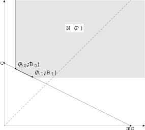
Let be given, and denote by the weight Moreover, let be a -homogeneous polynomial. Then its Newton diagram is a compact interval joining two vertices (which may coincide), where we shall assume that
Moreover, let be a change of coordinates of the form and (with ), if or and if (with ). Denote by the polynomial Then is -homogeneous of the same degree as and its Newton diagram is an interval of the form with
Assume either
-
(i)
that the interval lies in the closed half-space above the bisectrix, i.e., for every (Figure 1),
-
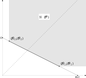
(ii)
or that the point lies above or on the bisectrix, i.e., and where denotes again the maximal order of vanishing of along the unit circle and the distance.
Then the point lies in the closed half-space above the bisectrix and the point lies in the closed half-space below the bisectrix. In particular, the Newton diagram intersects the bisectrix (Figure 2)
Proof. We have to show that the conditions (i) or (ii) imply
| (3.1) |
Now, by Proposition 2.2, we can write in the form
| (3.2) |
where the ’s are the non-trivial distinct complex roots of the polynomial and the ’s are their multiplicities.
It is easy to read off from (3.2) that the vertices of the Newton polyhedron of are given by and where
| (3.3) |
and that
(compare also [5] ); here, we have put
Assume first that and Then, by (3.2), we have
| (3.4) |
By looking at the terms of lowest power of in (3.4), we see that i.e.,
so that We next identify the term of highest power of in (3.4) in order to determine .
If for every then hence
Assume next that coincides with a non-trivial root (which is then necessarily real). Then we obtain
| (3.5) |
Now, if condition (i) holds, then by (3.3) we have
| (3.6) |
which by Corollary 2.3 easily implies and if (ii) holds, then
which is equivalent to Thus both conditions imply that
| (3.7) |
so that (3.1) is satisfied.
There remains the case and with In this case,
| (3.8) |
where Our assumptions imply that either (3.6) holds, or that for every such that is real we have
| (3.9) |
Notice also that it may happen that or but at most for one and one and these indices must be different, since has non-degenerate Jacobian at
Now, if for every then
and if then
Moreover, if for every then
and if then
Using (3.6) respectively (3.9), it is easy to check that and in all cases.
Q.E.D.
Fix now a smooth function defined near the origin satisfying and
Choose with such that the principal face of the Newton polyhedron lies on the line Notice that is uniquely determined, unless is a vertex. In the latter case, we shall assume that Flipping coordinates and if necessary, we shall assume without loss of generality that Notice that then if and only if the principal face is non-compact; in this case, it is a half-line which lies on the horizontal line given by And, if then the principal face is compact and the principal part of is a -homogeneous polynomial of degree one.
Consider next a smooth local coordinate system at the origin given by and put
Flipping coordinates and if necessary,we may assume without loss of generality that satisfies for .
Therefore, we can write the functions in the form
| (3.10) |
where are smooth functions satisfying
Since separate scaling of the coordinates and does not change the Newton polyhedron, we may further assume that
Denote by the order of vanishing of at Then clearly We shall see that if i.e., if the function is flat at then the distance will not change under the change of coordinates, i.e.,
On the other hand, if is finite, then according to (3.10), the main term of is of the form with We therefore then introduce a second weight Then the -principal part of is given by which is -homogeneous of degree Recall that denotes the supporting line to the Newton polyhedron Notice that the line has slope and has slope The effect of the change of coordinates on the Newton diagram is then related to the interplay between these two homogeneities and in particular the relation between the slopes of the corresponding supporting lines.
We put if
Lemma 3.2.
In the situation described above, the following hold true:
a) Assume either that
-
(i)
, and either or (so that the line is less steep than the line ), or that
-
(ii)
and
Then
a) If (so that the line is steeper than the line ), then
In particular, if i.e., if the principal edge is non-compact, then the coordinates are adapted to
Proof. a) The case where and
In this case so that the principal face is a half-line lying on the horizontal line given by and . Moreover, is flat at the origin, i.e.,
| (3.11) |
for every In view of the structure of the Newton polyhedron that we assume, it is easy to see that then can be written in the form
where and are smooth functions and and where are flat functions at the origin. Moreover, This implies that
for some smooth function and where and where is flat at the origin. Since by the product rule and (3.11) this easily implies that and if or if and so that but no lattice point below or to the left of this point. This shows that
b) The case where and either or and
Let us first state some general observation. If denotes the -principal part of then it is easily seen, e.g., by Lemma 2.1, that
so that
Moreover, is a -homogeneous polynomial, so that its Newton diagram is again a compact interval (possibly a single point). In case that this interval intersects the bisectrix too, then it is the principal face of Moreover, if has -degree one, then lies again on the line and consequently we have
Notice that the same conclusion holds true if are -homogeneous of any degree and if has the same -degree
Now, if then and thus, by (3.10), up to terms of higher -degree. Moreover, if or then also up to terms of higher -degree, so that Thus the reasoning above applies, and we see that
c) The case where and
In this case, the -principal part of is given by and the -principal part of is given by if and by if with if and only if
Choose such that the line is the supporting line to the Newton polyhedron and let be the -principal part of Then obviously Since the line is steeper than the line it is clear from the geometry of the Newton polyhedron that is a compact interval (possibly a single point) lying in the closed half-space above the bisectrix, i.e.,
Applying Lemma 3.1 to the -homogeneous polynomial we see that the Newton diagram of intersects the bisectrix. The principal face of lies therefore on the line and since this line is steeper then the line containing the principal face of it is clear from the geometry that
Finally, assume that Then either or and so we always have Therefore, the coordinates are adapted to
Q.E.D.
Theorem 3.3.
Let be a real analytic (respectively smooth ) function near the origin, with and Assume that the given coordinates are not adapted to Then all of the following conditions hold true:
-
(a)
The principal face of the Newton polyhedron is a compact edge.
It thus lies an a uniquely determined line with Flipping coordinates if necessary, we assume without loss of generality that
-
(b)
-
(c)
Any root of of maximal order on the unit circle lies away from the coordinate axes, and we have
In particular, there exists a unique non-trivial real root of the polynomial with multiplicity
Moreover, in this case, if we put then an adapted coordinate system for the principal part of is defined by The height of is then given by
Conversely, if all of the conditions (a) - (c) are satisfied, then the given coordinates are not adapted to the principal part of
Notice that for mixed homogeneous polynomials the theorem gives a necessary and sufficient condition for the adaptedness of the coordinates. We shall see later that the same is indeed true for general functions
Observe also that the root in (c) with multiplicity is the principal root of
Proof of Theorem 3.3. Assume that the coordinates are not adapted to Then there exists a smooth change of coordinates at the origin such that
| (3.12) |
Arguing similarly as in the proof of Lemma 3.2, we may assume that satisfies (3.10), with
Denote again by the order of vanishing of at and choose the weight as before in such a way that the principal face of lies on the line Again, assume that
From (3.12) and Lemma 3.2 it then follows that if then
and if then or In the latter case, by symmetry in the variables and let us assume without loss of generality that In particular, the principal face is compact, hence either a compact edge or a vertex. It is therefore an interval joining two vertices (which may coincide), i.e.,
We shall assume that Since this interval intersects the bisectrix we then have
| (3.13) |
In the sequel, let us write and consider the -homogeneous polynomial Its Newton diagram is given by the interval
We next show that To this end, assume to the contrary that so that satisfies condition (ii) in Lemma 3.1. Observe that the -principal part of is given by where and the -principal part of is given by unless (hence ) and when it is given by with Therefore, the -principal part of is given by
where and if and only if Lemma 3.1 then shows that the Newton diagram of intersects the bisectrix, so that the principal face of lies on the line hence This contradicts (3.12).
We have thus seen that our assumptions on imply that and Assuming these properties, write the principal part of according to Proposition 2.2 in the form
| (3.14) |
where the ’s are the non-trivial distinct complex roots of the polynomial and the ’s are their multiplicities.
Observe that clearly is contained in the half-plane so that Similarly, we see that Consequently, there must be an with real root so that Notice that this root is unique, by Corollary 2.3. Let us remark at this point that this excludes the possibility that the principal face of is a vertex, for then would be of the form so that had no non-trivial root. Consequently, is a compact edge.
We show that in this case the change of coordinates leads to adapted coordinates. To this end, we shall refer to the notation and results in the proof of Lemma 3.1, applied to
We have seen that the function representing in the new coordinates is again a -homogeneous polynomial, so that its Newton diagram is a compact interval , whose endpoints are given by and (3.5). Since now the order signs in (3.7) have to be replaced by i.e.,
This implies that the interval lies in the half-plane Consequently, the principal face of lies on the horizontal line hence . Since this face is non-compact, the coordinates are adapted, due to Lemma 3.2.
Notice, however, that the same change of coordinates will in general not lead to an adapted coordinate system for – this may require further, higher order terms in in addition to
Finally, assume conversely that all of the conditions (a) - (c) are satisfied. Then the coordinates are not adapted to since, as we have seen, we can change coordinates for in such a way that, in the new coordinates the distance is given by This concludes the proof of Theorem 3.3.
Q.E.D.
As a corollary, we obtain the following characterization of the height in case of a -homogeneous polynomial.
Corollary 3.4.
Let be a -homogeneous polynomial as in Proposition 2.2. Then
Proof.
We adopt the notation from Proposition 2.2. If then the coordinates are adapted to and by Corollary 2.3 (a) and (2.9) we have
So, assume next that Then, according to Corollary 2.3 (b), there is at most one real root of on the unit circle with multiplicity
If there is no such root, then and so the coordinates are adapted. This shows that
If there is such a root, and if it lies on one of the coordinate axes, then or hence and the claim follows. We may thus assume that the root does not lie on a coordinate axis, so that Then which implies that the principal face of the Newton polyhedron of must be a compact edge. Then, by Theorem 3.3, the coordinates are not adapted to and Since the conclusion follows also in this case.
Q.E.D.
4. The real analytic case
In this section we prove that if is a real analytic function then there exists an analytic coordinate system which is adapted to This coordinate system can be described in terms of the Puiseux series expansion of the roots of the equation
4.1. Description of the Newton polyhedron in terms of the roots.
Assume again to be real analytic and real valued. By the Weierstraß preparation theorem we can then write
near the origin, where is a pseudopolynomial of the form
and are real analytic functions satisfying . Observe that the Newton polyhedron of is the same as that of We shall also assume without loss of generality that is a non-trivial function, so that the roots of the equation considered as a polynomial in are all non-trivial.
Following [5], it is well-known that these roots can be expressed in a small neighborhood of as Puiseux series
where
with strictly positive exponents and non-zero complex coefficients and where we have kept enough terms to distinguish between all the non-identical roots of
By the cluster we shall designate all the roots , counted with their multiplicities, which satisfy
| (4.1) |
for some exponent . We also introduce the clusters by
Each index or varies in some finite range which we shall not specify here. We finally put
Let be the distinct leading exponents of all the roots of Each exponent corresponds to the cluster so that the set of all roots of can be divided as . Then we may write
where
We introduce the following quantities:
| (4.2) |
Notice that is just the number of all roots with leading exponent strictly greater than (where we here interpret the trivial roots corresponding to the factor in our representation of as roots with exponent ).
If denotes the total number of all roots of away from the axis including the trivial ones and counted with their multiplicities, then we can also write
| (4.3) |
Then, similarly as for the reduced Newton diagram in [5], the vertices of the Newton diagram of are the points and the Newton polyhedron is the convex hull of the set .
Notice also that
Let denote the line passing through the points and It is easy to see that it is given by
where This implies that
| (4.5) |
which in return is the reciprocal of the slope of the line The line intersects the bisectrix at the point where
Moreover, the vertical edge of the Newton polyhedron, which passes through the point intersects the bisectrix at and the horizontal edge, which passes through the point intersects the bisectrix at We therefore conclude that the distance is given by
Finally, fix and let us determine the -principal part of corresponding to the supporting line To this end, observe that has the same -principal part as the function
Moreover, the -principal part of is given by if and by if This implies that
| (4.6) |
In view of this identity, we shall say that the edge is associated to the cluster of roots We collect these results in the following lemma.
Lemma 4.1.
4.2. Existence of adapted coordinates in the analytic setting.
Theorem 4.2.
Let be a non-trivial real valued real analytic function defined on a neighborhood of the origin in with . Choose such that the principal face of the Newton polyhedron of lies on the line Without loss of generality, we may assume that . Then there exists a real analytic function of near the origin with such that an adapted coordinate system for near is given by
The function can in fact be chosen as one of the roots, respectively a leading partial sum of the Puiseux series expansion of one of the roots, of the equation considered as an equation in
Notice that Theorem 4.1 was proved by A.N. Varchenko in [7]. But, his proof is based on H. Hironaka’s [3] deep theorem on the resolution of singularities. We shall give a more elementary proof of Varchenko’s theorem, based on the Puiseux series expansion of roots of which in fact gives an explicit description of an adapted coordinate system in terms of these roots.
Proof. We may and shall assume without loss of generality that If the coordinate system is adapted, then we can choose According to Theorem 3.3, this applies in any of the following three cases:
-
(a)
The principal face is unbounded. Since we are assuming that by Lemma 4.1 this means that i.e., that
(4.8) -
(b)
consists of a vertex. Then choose so that This happens iff
(4.9) -
(c)
is a compact edge but
(4.10) or
(4.11)
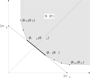
There remains the case where the principal face is a compact edge ( ), and there is an index such that
| (4.12) |
(Figure 3). Notice that in view of Corollary 2.3 the index is unique, and is the principal root of
We then apply an algorithm due to Varchenko [7].
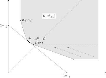
Step 1 (Figure 4). We apply the real change of variables given by and put again In order to describe the effect of this change of variables to the Newton polyhedron, let us denote all quantities associated to with a superscript .
Observe first that the roots of are of the form
| (4.13) |
respectively (namely those corresponding to the trivial roots of ). This shows that the leading exponents
of these roots are given by for with the same multiplicities (where denotes the cluster of roots associated to the index ).
For the vertices of we thus obtain from (4.2), (4.3) that
| (4.14) |
Moreover, any root belonging to a cluster with is transformed into a root with leading exponent Finally, if belongs to then either the leading exponent of is (namely if ), or it is of the form We therefore distinguish two cases.
Case 1.
Then there exists at least one root with leading exponent so that Moreover, since is the number of roots with leading exponent strictly greater than we see that Similarly, the number is the same as the number of roots with leading exponent strictly greater than or equal to but then with index hence This implies In combination, we thus have
| (4.15) |
But, estimate (4.12) is equivalent to so that the edge which lies on the same line as the edge and has the same left vertex, is not the principal face of the Newton polyhedron of Finally, it is evident from (4.13) that in this case if (unless there is no cluster with )
This shows that in this case the principal face of is either associated to a cluster of roots which corresponds to a cluster of roots in the original coordinates, or is a horizontal, unbounded edge (so that the new coordinates are adapted).
Case 2.
Then there is no root with leading exponent and so again the conclusion stated at the end of the previous case applies.
In both cases we see that the principal face of the new Newton polyhedron will be less steep than the one of so that
Subsequent steps. Now, either the new coordinates are adapted, in which case we are finished. Or we can apply the same procedure to Composing the change of coordinates from the first step with the one from the second step, we see that we then can find a change of coordinates of the form
with and such that the following holds: If the function expresses the function in the new coordinates, then the principal face of the Newton polyhedron of is either associated to a cluster of roots which corresponds to a cluster of roots in the original coordinates, or is a horizontal, unbounded edge (so that the new coordinates are adapted).
Now, if we iterate this procedure, then either this procedure will stop after finitely many steps, or it will continue infinitely. If it stops, it is clear that we will have arrived at a new, adapted coordinate system of the form
and Theorem 4.2 holds with a polynomial function
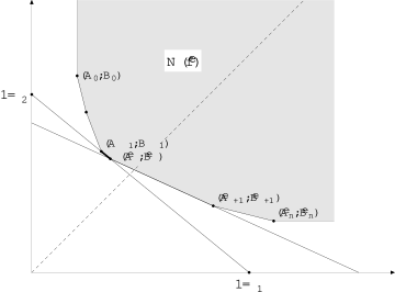
Final step (Figures 5,6). Assume that the procedure does not terminate. Then, in each further step we pass to a new Newton diagram with a principal face associated to a cluster of roots (in the old coordinates) which is a sub-cluster of the previous cluster In particular, the corresponding muliplicities form a decreasing sequence, so that they eventually must become constant. Choose such that for every Replacing the original coordinate system by the one obtained in the -th step, we may assume without loss of generality that i.e.,
| (4.16) |
This clearly implies that for every and that each of the clusters contains exactly one and the same root (of multiplicity ), namely
| (4.17) |
(so that in fact for every ) Moreover, our procedure shows that all cofficients in this series must be real, and all exponents positive integers, so that is a real valued, real analytic function of
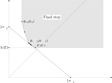
If we apply our first change of coordinates in this situation, then we see that the leading exponents of the new roots are given by and in Case 1, and by and in Case 2. Moreover, it is clear from our discussion that the last edge, associated to the cluster of roots with biggest leading exponent must be the principal edge. Moreover, in the new coordinates the function can have no vanishing root, since such a root would have corresponded to a root which, by (4.17), cannnot exist in the cluster
By passing to these new coordinates, we may therefore assume in addition to (4.16) that the cluster is the cluster associated to the principal face of the Newton polyhedron of and that i.e., that
| (4.18) |
The Newton polyhedron of thus has vertices and the principal edge is given by where, according to (4.2), (4.16),
| (4.19) |
Let us finally apply the change of coordinates The non-zero roots of are then given by with for some and they have the same multiplicities and leading exponents as the corresponding roots In view of (4.2), the vertices of the Newton diagram are thus given by the points i.e., the effect of the change of coordinates on the Newton diagram is the removal of the last vertex Since, by (4.19), the vertex lies above the bisectrix, we see that the principal face of is the horizontal half-line emerging from the point along the line a non-compact set. According to Theorem 3.3, the coordinates are thus adapted to and the height is given by
| (4.20) |
Q.E.D.
The proof suggests the following definitions. If
is any root of (more precisely, of ), then any leading part
with which is real analytic, i.e, where all exponents appearing in this series are positive integers, will be called an analytic root jet.
We have seen that the function constructed by Varchenko’s algorithm in a unique way is indeed an analytic root jet, which we call the principal root jet.
Our proof even reveals that the conditions (a) - (c) in Theorem 3.3 are necessary and sufficient for the adapteness of the given coordinate system for arbitrary analytic functions In the statements of the following corollaries we shall always make the following
General Assumptions. The function is a real valued real analytic function defined on a neighborhood of the origin in with . Choose such that the principal face of the Newton polyhedron of lies on the line and assume that .
Corollary 4.3.
The given coordinates are not adapted to if and only if the conditions (a) - (c) in Theorem 3.3 are satisfied. In particular, the given coordinates are adapted to if and only if they are adapted to the principal part of
Moreover, we always have
Proof. The necessity of these conditions for non-adaptedness has been proved in Theorem 3.3. Assume conversely that (a) - (c) hold true. In that case, we have seen in the proof of Theorem 4.2 that there exists a change of coordinates which strictly increases the height, so that the original coordinates are not adapted.
Since the conditions (a) - (c) depend in fact only on we see in particular that the given coordinates are adapted to if and only if they are adapted to the principal part of
Finally, if the coordinates are adapted to (hence also to ), then we clearly have Otherwise, the proof of Theorem 4.2 shows that the first change of coordinates that we considered reduces the principal edge to the shorter interval (possibly of length zero) on the same line, but lying above the bisectrix. Notice that the coordinates are already adapted to the principal part and that, by (4.15), (4.12) and Theorem 3.3, we have
But, the point will be contained in the Newton diagrams of associated to all subsequent systems of coordinates that we constructed by our algorithm (compare (4.14), applied to the coordinates ), which means that the principal face of in our final, adapted coordinate system must lie in the half-space so that
Q.E.D.
Corollary 4.4.
a) We can always find a change of coordinates at of the form such that the coordinates are adapted to and the following hold true:
If the principal face is compact and lies on the line with then is a polynomial of degree strictly less than
This applies in particular, if the height of is a non-integer rational number.
b) There always exists a change of coordinates of the form at the origin, with a polynomial function such that in the new coordinates we have Here, we have again put
Proof. Indeed, the algorithm that we devised in the proof of Theorem 4.2 in order to construct an adapted coordinate system shows that we can arrive at an adapted coordinate system with a polynomial function unless we have to choose for one of the roots with infinitely many non-trivial terms in its Puiseux series expansion. In the latter case, the principal face in the adapted coordinate system that we constructed is non-compact and the height is an integer, as we have seen. Thus, if the principal face in the adapted coordinate system is compact, the algorithm must terminate after a finite number of steps. And, in Step 1, the degree of the polynomial used in the change of coordinates is given by where by (4.10) is just the inverse of the slope of the principal edge of the Newton polyhedron of However, the proof shows that the slope of the principal face strictly decreases by the change of coordinates in Step 1, and the same applies to all subsequent steps. If we apply this to the last change of coordinates before achieving adapted coordinates, we see that the function is a polynomial of degree This proves a).
Moreover, in the case where our algorithm does not terminate, after finitely steps in our algorithm (which all consist of polynomial changes of coordinates), we may assume that the polynomial corresponding to the principal face of the Newton diagram has a unique root of multiplicity (compare (4.16), (4.17) and (4.20)). If we choose the coordinates which we obtain at this stage, we then have so that also b) is proven.
Q.E.D.
5. The smooth case
We shall finally extend Theorem 4.2 to the smooth setting.
Theorem 5.1.
Let be a real valued smooth function of finite type defined on a neighborhood of the origin in with . Choose such that the principal face of the Newton polyhedron of lies on the line Without loss of generality, we may assume that . Then there exists a smooth function of near the origin with such that an adapted coordinate system for near is given by
Proof. We proceed in a very similar way as in the analytic setting, adopting also the same notation. If the coordinates are adapted to then we may choose and are finished.
Otherwise, again by Theorem 3.3, the principal face is a compact edge. Moreover, we have and Let us then choose a real root of the principal part of of maximal multiplicity i.e., the principal root. Then again by Theorem 3.3,
Step 1. We apply the real change of variables given by and put Let us again endow all quantities associated to with a superscript . Now, if the coordinates are adapted to we choose and are finished.
Otherwise, the principal face is a compact edge, and we have and Recall that the principal part of is -homogeneous of degree one. We claim that
| (5.1) |
Indeed, recall that the effect of our change of coordinates on the Newton polyhedron is such that it preserves all lines Let us therefore choose so big that we have for every point lying on any such line passing through any point in the Newton diagram of and denote by the Taylor polynomial of order of Then it is clear that and have the same principal faces and parts, and the same applies to and I.e., we have and We can therefore apply our results for the analytic case to the polynomial function and obtain (5.1).
This argument also shows that the change of coordinates increases the distance, i.e.,
Subsequent steps. Now, either the new coordinates are adapted, in which case we are finished. Or we can apply the same procedure to etc.. In this way, we obtain a sequence of functions with and which can be obtained from the original coordinates by means of a change of coordinates of the form
with positive integers and real coefficients Moreover, if denotes the maximal order of vanishing of the principal part of along the unit circle then we have
Either this procedure will stop after finitely many steps, or it will continue infinitely. If it stops, say, at the -th step, it is clear that we will have arrived at an adapted coordinate system with a polynomial function
Final step. Assume that the procedure does not terminate. Since the maximal multiplicities of the roots of the principal part of form a decreasing sequence, we find again some such that for every By comparing with the effect of the change of coordinates in each step of order with the effect on the Taylor polynomial of sufficiently high degree, we see from the corresponding result (4.18) in the analytic case that the principal part of is of the form
where It is mixed homogeneous of degree one with respect to the weight given by
so that, for
| (5.2) |
Now, according to the classical Borel lemma, we can find a smooth function near the origin whose Taylor series is the formal series Consider the smooth change of coordinates given by and put We claim that the coordinates are adapted to
Indeed, we have
where has the Taylor series In view of (5.2), this show that
| (5.3) |
where is a smooth function consisting of terms of -degree strictly bigger than one, for every i.e.,
| (5.4) |
Since as this implies that Moreover, if then the left-hand side of (5.4) is bounded by if so that we must have In combination, (5.3) and (5.4) show that the Newton polyhedron of contains the point but nor further point on the left to this point on the line and that all other points of are contained in the open half-plane above this line. Since this shows that the principal face of is the unbounded horizontal half-line given by hence the coordinates are adapted to
Q.E.D.
The following corollary is immediate from the proof of Theorem 5.1 and the proofs of the Corollaries 4.3 and 4.4, which carry over to the smooth setting.
Corollary 5.2.
Let be a real valued smooth function of finite type defined on a neighborhood of the origin in with . Then the height is a rational number.
ACKNOWLEDGEMENT
We wish to thank Michael Kempe for his support in creating the graphics included in this article.
References
- [1] V.I. Arnol’d, Remarks on the method of stationary phase and Coxeter numbers, Uspekhi Mat. Nauk. 1973, 28;5, 17-44. English transl. Russ. Math. Surv. 28:5 (1973), 19-58.
- [2] V.I. Arnol’d, C.M. Guseyn-zade, and A.N. Varchenko, Singularities of Differentiable Maps, Vol. II. Monodromy and asimptotic of Integrals. Nauka, Moscow (1984), English transl. Birhauser, Boston. Basel. Berlin. 1988.
- [3] H. Hironaka, Resolution of singularities of an algebraic variety over a field of characteristic zero. I., II. Ann. Math., (2), 79 (1964), 109-326.
- [4] I.A. Ikromov, M. Kempe, and D. Müller, Damped oscillatory integrals and boundedness of maximal operators associated to mixed homogeneous hypersurfaces, Duke Math. Journal, Vol. 126, No. 3 (2005), 471-490.
- [5] D. H. Phong and E. M. Stein, The Newton polyhedron and oscillatory integral operator, Acta Math. 179(1) (1997), 105-152.
- [6] E. M. Stein, Harmonic analysis: real-variable methods, orthogonality, and oscillatory integrals, Princeton Mathematical Series, vol. 43, Princeton University Press, Princeton, NJ, 1993.
- [7] A. N. Varchenko, Newton polyhedra and estimates of oscillating integrals, Funct. anal. and Appl. 10(3) (1976), 175-196.