Ab initio statistical mechanics of surface adsorption
and desorption: I. H₂O on MgO (001) at low coverage

Abstract

We present a general computational scheme based on molecular dynamics (m.d.) simulation for calculating the chemical potential of adsorbed molecules in thermal equilibrium on the surface of a material. The scheme is based on the calculation of the mean force in m.d. simulations in which the height of a chosen molecule above the surface is constrained, and subsequent integration of the mean force to obtain the potential of mean force and hence the chemical potential. The scheme is valid at any coverage and temperature, so that in principle it allows the calculation of the chemical potential as a function of coverage and temperature. It avoids all statistical mechanical approximations, except for the use of classical statistical mechanics for the nuclei, and assumes nothing in advance about the adsorption sites. From the chemical potential, the absolute desorption rate of the molecules can be computed, provided the equilibration rate on the surface is faster than the desorption rate. We apply the theory by ab initio m.d. simulation to the case of H₂O on MgO (001) in the low-coverage limit, using the Perdew-Burke-Ernzerhof (PBE) form of exchange-correlation. The calculations yield an ab initio value of the Polanyi-Wigner frequency prefactor, which is more than two orders of magnitude greater than the value of $10^{13}$ s^-1 often assumed in the past. Provisional comparison with experiment suggests that the PBE adsorption energy may be too low, but the extension of the calculations to higher coverages is needed before firm conclusions can be drawn. The possibility of including quantum nuclear effects by using path-integral simulations is noted.

1 Introduction

Ab initio modelling based on density functional theory (DFT) has had a major impact on the understanding of molecular adsorption and desorption at surfaces [1, 2]. However, most of this modelling has been of the static kind, in which structural relaxation is used to calculate the energies of chosen adsorbate geometries. For the interpretation of some types of experiment, static calculations may suffice, but in many practical situations entropy effects cannot be ignored. This is clearly true when one considers surface phase diagrams or adsorption isotherms, but it is also true for rate processes such as thermal desorption. In a recent short publication [3], we showed the possibility of using DFT molecular dynamics simulation to calculate absolute desorption rates, with full inclusion of all entropy effects. Our aims here are to describe the general theory underlying that work, to outline its relevance to the calculation of adsorption isotherms, to present the simulations themselves in more detail, and to indicate several developments that we plan to explore in future papers.

Although most DFT surface modelling has been static, the general idea of ab initio statistical mechanics (AISM) applied to condensed matter goes back well over 10 years [4, 5]. Over that period, methods for calculating the ab initio free energy of liquids and anharmonic solids have become well established [6, 7, 8]. In surface science, one of the earliest publications describing a form of AISM was that of Stampfl et al. [9] on the O/Ru (0001) system, in which they successfully calculated thermal desorption spectra, heat of adsorption and the surface phase diagram.

All previous AISM work that we know of on surface adsorbates has been based on lattice-gas schemes, which we specifically wish to avoid here. To make this point clear, we recall that there are two fundamentally different approaches to the statistical mechanics of adsorbates. In lattice gas theories, it is assumed from the outset that the adsorbate atoms or molecules (for brevity, we shall simply say ‘molecules’) can occupy only specified surface sites. Calculations are then formulated in terms of the occupancies of these sites and transition rates between them, the model parameters being fixed either by appeal to experiment or (more recently) to DFT calculations. A completely different approach is to regard the adsorbate molecules as forming a two-dimensional fluid interacting with the substrate. The methods we shall describe resemble the second approach, and are also close to the AISM methods developed for bulk liquids. A crucial point is that these bulk AISM methods are designed to deliver free energies or chemical potentials that are free of statistical-mechanical errors (more precisely, these errors can be systematically reduced to any desired tolerance) [10, 11]. Here, we have the same aim for the AISM of adsorbates: the statistical mechanical errors should be systematically controllable, so that the only remaining error is due to the DFT exchange-correlation approximation. In a lattice-gas approach, by contrast, the adoption of a discrete set of adsorption sites constitutes an approximation that is difficult to eliminate, and this is why we avoid this approach.

Coming to specifics, the modelling techniques that we wish to develop should allow the calculation of the chemical potential of a system of adsorbate molecules on the surface of a material at any coverage and temperature, starting from a given DFT exchange-correlation functional. We focus particularly on the chemical potential, since this is the key to calculating all other thermodynamic properties of the adsorbate, as well as the thermal desorption rate measured in temperature programmed desorption (TPD) experiments [12]. The techniques should not assume in advance anything about the sites occupied by the adsorbate molecules, or about their orientations, and should not rely on the harmonic approximation for any of the degrees of freedom. Ultimately, though not in this paper, we should like to be able to treat molecules that dissociate and undergo chemical reactions. We want to be able to include quantum nuclear effects, if necessary. Although we assume for the moment that the ab initio total energy function is provided by DFT, we recognise that DFT is often inaccurate, and we want the techniques to be generalisable to more accurate ab initio methods, such as quantum Monte Carlo [13] or high-level quantum chemistry.

We present in the next Section a theoretical scheme which we believe will be capable of allowing many of these aims to be accomplished. Our strategy is to consider the system consisting of the adsorbate molecules on the surface in complete thermal equilibrium with the gas phase. All molecules in the system, including those in the substrate, are treated on an equal footing. In this situation, there is a distribution $\bar{\rho}(z)$, giving the probability of finding adsorbate molecules a distance $z$ from the surface. This distribution can be expressed in terms of a potential of mean force (PMF): $\bar{\rho}(z)=A\exp(-\phi(z)/k_{\rm B}T)$, and the PMF $\phi(z)$ is the integral with respect to $z$ of the mean force $\langle{\cal F}_{z}\rangle_{z}$ acting on the adsorbate molecules when they are constrained to be at distance $z$ from the surface. We shall show how these simple relationships allow the calculation of the chemical potential of the adsorbate. We note that the same relationships also yield the absolute rate of thermal desorption as a function of coverage and $T$, provided all equilibration rates on the surface are faster than the desorption rate. We shall show that, under appropriate conditions, the theory yields the widely used Polanyi-Wigner equation [14], according to which the rate of change of adsorbate coverage $\theta$ (molecules per adsorption site) in a TPD experiment is given by:

$$d\theta/dt=-f\theta^{n}\exp(-\Delta E/k_{\rm B}T)\;,$$ (1)

where $\Delta E$ and $n$ are the activation energy and reaction order for desorption, and $f$ is a frequency prefactor. In the analysis of experimental TPD data [15, 16], $f$ is commonly treated as an empirical adjustable parameter, but the theory we present is capable of yielding ab initio values for $f$.

The practical application of the scheme reported in this paper (Sec. 3) consists of DFT simulations of the H₂O molecule on the perfect MgO (001) surface at several temperatures in the limit of zero coverage. We confine ourselves here to zero coverage, even though the theory is equally valid at all coverages, simply because the practical sampling requirements are easier to satisfy in this case. The target we set ourselves is to calculate the chemical potential of the adsorbate molecule in thermal equilibrium, with complete inclusion of entropy effects, to an accuracy of better than 50 meV for the chosen exchange-correlation functional. We shall see that even at low coverage entropy effects are very important, and increase the frequency prefactor for thermal desorption by over two orders of magnitude in the temperature range of practical interest. In Sec. 4, we discuss the practical problems involved in doing calculations at higher coverages, and possible ways of overcoming them; we also discuss the generalisation to include quantum nuclear effects, using DFT path-integral techniques. Our conclusions are summarised in Sec. 5

2 Theory and techniques

We begin our outline of theory and techniques by describing the statistical mechanical relationships that allow us to calculate the chemical potential of adsorbed molecules using PMF techniques. We then summarise the arguments that allow the thermal desorption rate to be deduced from this chemical potential in the case of fast equilibration. At the end of this Section, we discuss the practical issues in calculating the PMF, and we provide technical details of the DFT molecular dynamics techniques used to perform our simulations of the isolated H₂O molecule on the MgO (001) surface.

2.1 Calculation of the chemical potential using PMF

The adsorbate molecules are all identical to each other, and are called species A; the atoms in the solid are called species B. We consider first the situation where A-molecules in the gas phase are in complete thermal equilibrium with those adsorbed on the surface. We assume that A-molecules cannot penetrate into the bulk. The situation we envisage is adsorption of molecules on the surface of a perfect crystal, with this surface corresponding to a particular crystal plane and being free of defects. This being so, we can draw a “reference plane” parallel to the surface, whose position is such that if translated outward by a few lattice spacings along the surface normal it would be entirely in the gas phase, and if translated inward by a similar amount it would be entirely in the bulk. The origin of coordinates lies in this reference plane, with the $z$-axis pointing along the outward normal.

When the entire system is in thermal equilibrium at a given temperature $T$ and a given chemical potential of the A-molecules, there is a density $\rho_{0}$ (number per unit volume) of A-molecules in the gas phase, and a surface density $\sigma$ (number per unit area) on the surface. In order to make $\sigma$ well defined, we have to decide what is meant by an A-molecule being “on the surface”. In order to do this, we define a “monitor” point for each A-molecule. If the molecule is an atom, this monitor point is just the position of the nucleus. If it is a molecule, it could be chosen as the position of a specified nucleus, or as the the centre of mass, or in some other way. The particular choice of monitor point will not (significantly) affect any of the physical results of interest. To separate A-molecules in the gas from those on the surface, we define a “transition plane”, which is parallel to the reference plane, but displaced from it by the $z$-displacement $z_{0}$. An A-molecule is counted as on the surface if the $z$-coordinate of its monitor point is less than $z_{0}$, and in the gas phase otherwise. To ensure that the value of $\sigma$ does not depend significantly on the position of the transition plane, we choose $z_{0}$ so that the interaction of an A-molecule with the solid is negligible for $z\geq z_{0}$.

Since we have full thermodynamic equilibrium, the chemical potentials $\mu_{\rm gas}(\rho_{0},T)$ and $\mu_{\rm ads}(\sigma,T)$ in the gas phase and on the surface must be equal. We are primarily interested in situations where $\rho_{0}$ is so low that interactions between A-molecules in the gas are negligible. It is then convenient to express $\mu_{\rm gas}$ as:

$$\mu_{\rm gas}(\rho_{0},T)=k_{\rm B}T\ln(\rho_{0}\Lambda^{3})+\mu_{\rm gas}^{\dagger}(T)\;,$$ (2)

where the first term on the right is the chemical potential of a perfect gas of structureless particles, whose mass $M_{\rm A}$ is equal to that of the A-molecules, and $\Lambda$ is the thermal wavelength $\Lambda=\left(h^{2}/2\pi M_{\rm A}k_{\rm B}T\right)^{1/2}$. If the A-molecules are atoms, then $\mu_{\rm gas}^{\dagger}(T)=0$, but if they are molecules, $\mu_{\rm gas}^{\dagger}(T)$ represents the $T$-dependent contribution to $\mu_{\rm gas}(\rho_{0},T)$ from internal vibrations and rotations. In a similar way, it is convenient to express $\mu_{\rm ads}(\sigma,T)$ as:

$$\mu_{\rm ads}(\sigma,T)=k_{\rm B}T\ln(\sigma\Lambda^{3}/d)+\mu_{\rm ads}^{\dagger}(\sigma,T)\;.$$ (3)

where $d$ is an arbitrary fixed length. By analogy with the gas-phase chemical potential, the first term on the right represents the chemical potential of a gas of structureless particles of mass $M_{\rm A}$ confined to the surface region. The “excess term” $\mu_{\rm ads}^{\dagger}(\sigma,T)$ depends, of course on the value chosen for $d$, but this is a convenient way to write $\mu_{\rm ads}$, because in the limit where quantum nuclear effects can be ignored, $\mu_{\rm ads}^{\dagger}(\sigma,T)$ is then independent of Planck’s constant. This way of separating $\mu_{\rm ads}$ is particularly helpful in the limit of low coverage, $\sigma\rightarrow 0$, when $\mu_{\rm ads}^{\dagger}$ becomes independent of $\sigma$ and includes the adsorption energy of A-molecules, as well as the entropy effects due to translations, vibrations and (hindered) rotations. For non-zero $\sigma$, $\mu_{\rm ads}^{\dagger}$ also includes the energetic and entropic effects of adsorbate-adsorbate interactions. With these definitions, the combination of eqns (2) and (3) with the equilibrium condition $\mu_{\rm gas}=\mu_{\rm ads}$ gives:

$$\sigma/\rho_{0}=d\exp\left[\beta\Delta\mu^{\dagger}(\sigma,T)\right]\;,$$ (4)

where $\Delta\mu^{\dagger}\equiv\mu_{\rm gas}^{\dagger}-\mu_{\rm ads}^{\dagger}$. We refer to $\Delta\mu^{\dagger}$ as the “excess chemical potential difference” (ECPD). The adsorption isotherm ($\sigma$ as a function of $\rho_{0}$ or gas pressure at constant $T$) can then be found by solving eqn (4) for $\sigma$. In calculating the thermodynamic properties of the adsorbate on the surface, it is therefore convenient to focus on the quantity $\Delta\mu^{\dagger}(\sigma,T)$.

We shall need later the relation between $\Delta\mu^{\dagger}$ and the isosteric heat of adsorption $h_{\rm iso}$, which can be defined as the negative slope of $\ln(\rho_{0})$ plotted against $1/T$ at constant surface density $\sigma$. From eqn (4), we have:

$$h_{\rm iso}=-\left(\frac{\partial}{\partial\beta}\ln(\rho_{0}d/\sigma)\right)_{\sigma}=\left(\frac{\partial}{\partial\beta}\left(\beta\Delta\mu^{\dagger}\right)\right)_{\sigma}\;.$$ (5)

To develop a strategy for calculating $\Delta\mu^{\dagger}$, we consider the spatial distribution of A-molecules in thermal equilibrium. Let $\rho({\bf r})\,d{\bf r}$ represent the probability of finding the monitor point of any A-molecule in volume element $d{\bf r}$ at position ${\bf r}$. If ${\bf r}_{n}$ is the dynamical variable representing the position of the monitor point of A-molecule $n$ and there are $\nu$ A-molecules in the system, then $\rho({\bf r})$ is:

$$\rho({\bf r})=\left\langle\sum_{n=1}^{\nu}\delta({\bf r}-{\bf r}_{n})\right\rangle\;,$$ (6)

where $\langle\,\cdot\,\rangle$ denotes thermal average. When ${\bf r}\equiv(x,y,z)$ is near the surface, $\rho(x,y,z)$ depends on $x$ and $y$ as well as $z$, and exhibits the translational periodicity of the surface. We are not interested here in the dependence on $x$ and $y$, so we consider the distribution $\bar{\rho}(z)$, which is the spatial average of $\rho(x,y,z)$ over $x$ and $y$. For $z$ far from the surface, $\bar{\rho}(z)$ is equal to the gas number density $\rho_{0}$, but in the region of the surface, $\bar{\rho}(z)$ will have a large peak (or perhaps more than one peak), due to A-molecules adsorbed on the surface. With the position $z_{0}$ of the “transition plane” chosen as above, this peak is entirely in the region $z<z_{0}$, and for $z\geq z_{0}$, $\bar{\rho}(z)$ is very close to $\rho_{0}$. The surface density $\sigma$ of adsorbed molecules is the integral of $\bar{\rho}(z)$ over the region $z<z_{0}$. It is convenient to work with the distribution $y(z)\equiv\bar{\rho}(z)/\rho_{0}$, which is normalised so that $\lim_{z\rightarrow\infty}y(z)=1$. Then we have:

$$\sigma/\rho_{0}=\int_{-\infty}^{z_{0}}dz\,y(z)\;.$$ (7)

From this, we see that $y(z)$ is closely related to the ECPD $\Delta\mu^{\dagger}$. In fact, from eqn (4):

$$\exp\left[\beta\Delta\mu^{\dagger}(\sigma,T)\right]=\frac{1}{d}\int_{-\infty}^{z_{0}}dz\,y(z)\;.$$ (8)

Standard m.d. simulation can be used to calculate the unnormalised distribution $\bar{\rho}(z)\equiv\rho_{0}y(z)$ in the region of $z$ where the adsorbed molecules spend most of their time. Accumulation of a histogram for the probability distribution of $z$ suffices for this purpose. However, in order to perform the integral in eqn (8) we need the normalised distribution $y(z)$, and for this, the entire region $z<z_{0}$ must be sampled. Under most circumstances, simple accumulation of a histogram is not a practicable way of doing this, because the probability of adsorbed molecules sampling the region $z\sim z_{0}$ is so small. There are several well known techniques for overcoming this “rare-event” problem. The technique employed in the present work uses the potential of mean force (PMF) [17]. In this approach, $y(z)$ is expressed in terms of a PMF $\phi(z)$, which plays the role of a $z$-dependent free energy:

$$y(z)=\exp\left[-\beta\phi(z)\right]\;.$$ (9)

By standard arguments, the $z$-derivative $d\phi/dz$ is equal to minus the thermal average of the $z$-component of the force acting on the monitor point of a chosen A-molecule. Denoting by $\langle{\cal F}_{z}\rangle_{z}$ the thermal average of the $z$-component of the force acting on the molecule when the $z$-component of its monitor point is constrained to have the value $z$, we then have:

$$\phi(z)=\int_{z}^{\infty}dz^{\prime}\,\langle{\cal F}_{z}\rangle_{z^{\prime}}\;,$$ (10)

where $\langle{\cal F}_{z}\rangle_{z}$ is counted positive if directed outwards. Combining eqns (8) and (9), we obtain a formula for the ECPD $\Delta\mu^{\dagger}(\sigma,T)$ in terms of the mean force:

$$\Delta\mu^{\dagger}(\sigma,T)=k_{\rm B}T\ln\left\{\frac{1}{d}\int_{-\infty}^{z_{0}}dz\,e^{-\beta\phi(z)}\right\}=k_{\rm B}T\ln\left\{\frac{1}{d}\int_{-\infty}^{z_{0}}dz\,\exp\left[-\beta\int_{z}^{\infty}dz^{\prime}\,\langle{\cal F}_{z}\rangle_{z^{\prime}}\right]\right\}\;.$$ (11)

The physical content of this expression is that the ECPD is determined by the reversible work (integral of mean force) performed on transporting the molecule from one phase to the other. The calculation strategy is to evaluate the mean force $\langle{\cal F}_{z}\rangle_{z}$ as a time average in a series of constrained DFT m.d. simulations at a sequence of $z$ values, and to compute the mean force integral numerically. This strategy can in principle be applied at any temperature and coverage, provided ways can be found of achieving adequate statistical accuracy. It is one of the purposes of this paper to test the practical feasibility of the strategy.

We note in passing an alternative way of calculating $y(z)$, which should also be effective, namely umbrella sampling [18, 19]. In this, the probability distribution of the dynamical variable being sampled is deliberately biased by adding to the Hamiltonian a potential that acts on this variable. In the present case, we would add a potential $V_{\rm up}(z_{1})$ acting on the $z$-coordinate of the monitor point of a chosen molecule. It is an exact result of classical statistical mechanics that the probability distribution $\tilde{p}(z)$ of the chosen molecule is related to the distribution $y(z)$ in the absence of $V_{\rm up}$ by $\tilde{p}(z)=Ay(z)\exp(-\beta V_{\rm up}(z))$, where $A$ is a constant. If $V_{\rm up}(z)$ is appropriately chosen (in particular, if it is similar to $-\phi(z)$), $\tilde{p}(z)$ can be fully sampled over the required region $z<z_{0}$ by accumulation of a histogram, and $y(z)$ can then be recovered by multiplying by $\exp(\beta V_{\rm up}(z))$.

2.2 Thermal desorption rate

The rate at which molecules desorb from the surface when there is complete thermal equilibrium between gas and adsorbed molecules can be derived by standard detailed-balance arguments, which we recall briefly. (The arguments are well known [20], but we need to express them in a way that is consistent with the present notation.) According to elementary statistical mechanics, the outward flux $\kappa$ of molecules across the transition plane is $\kappa=\rho_{0}\left(k_{\rm B}T/2\pi M_{\rm A}\right)^{1/2}$, where we make a negligible error in setting the number density at the transition plane equal to $\rho_{0}$. If the sticking coefficient $S$ of molecules arriving from the gas phase is unity, then the flux $\kappa$ is entirely due to spontaneously desorbing molecules. But if $S<1$, then only the flux $S\kappa$ is due to spontaneous desorption. We denote by $\gamma$ the probability per unit time that a molecule spontaneously desorbs, so that $\gamma\sigma=S\kappa$. It follows from eqns (4) and (7) that:

$$\gamma = \left(\rho_{0}/\sigma\right)S\left(k_{\rm B}T/2\pi M_{\rm A}\right)^{1/2}=S\left(k_{\rm B}T/2\pi M_{\rm A}\right)^{1/2}\left/\int_{-\infty}^{z_{0}}dz\,y(z)\right.$$ (12)

$$= S\left(k_{\rm B}T/2\pi M_{\rm A}\right)^{1/2}\frac{1}{d}\exp\left[-\beta\Delta\mu^{\dagger}\right]\;.$$

Although eqn (12) is derived for conditions of complete thermal equilibrium, it may sometimes be correct for the desorption rate in a TPD experiment, even though this is an irreversible process. A necessary condition for it to be correct is that the rate of equilibration of the adsorbate on the surface be fast compared with the desorption rate $\gamma$. In general, the desorption of a molecule from the surface leaves behind a distribution of the remaining molecules that is not typical of thermal equilibrium. If the molecules in the region where the desorption happened do not have time to equilibrate before the next desorption occurs in this region, then the use of eqn (12) is no longer strictly correct. The equation can also fail for another reason. In a TPD experiment, the molecules are deposited on the surface at a very low temperature, and $T$ is steadily increased. If the rate of temperature increase is so fast that the adsorbate system has no time to equilibrate, then the desorption rate will be history dependent, and eqn (12) will fail, even at low coverage. In the simulations presented in Sec. 3, we shall study the relaxation rates associated with diffusion and reorientation of the H₂O molecule on MgO (001), in order to test the correctness of the formula for $\gamma$.

2.3 Practical calculation of PMF

It is clear from the foregoing theory that the primary quantity to be calculated is the mean force $\langle{\cal F}_{z}\rangle_{z}$, from which we obtain the PMF and chemical potential by integration. The calculation of $\langle{\cal F}_{z}\rangle_{z}$ by m.d. simulation of H₂O on MgO (001) raises a number of practical issues. We recall first that we are free to choose the molecular “monitor position” in different ways. In the present work, we choose it to be the position of the water O atom. At each time step of m.d., the electronic-structure calculation yields a Hellmann-Feynman force on the core of the water O exerted by the valence electrons and the other ionic cores. In constrained m.d. in which the $z$-coordinate of water O is held fixed, ${\cal F}_{z}$ is simply the $z$-component of this Hellmann-Feynman force. However, we note a disadvantage of this choice of monitor point, which is that ${\cal F}_{z}$ does not vanish even when the molecule is far from the surface, because the water O oscillates with the internal vibrational modes of the molecule. This means that time averaging is needed to calculate $\langle{\cal F}_{z}\rangle_{z}$, even when the constrained value of $z$ is far from the surface. This problem can be avoided, and the statistical efficiency somewhat improved, by choosing the monitor point to be the centre of mass of the molecule, as we shall discuss in detail in paper II.

Given our stated aim of calculating $\Delta\mu^{\dagger}$ correct to better than 50 meV for a chosen exchange-correlation functional, we need to give thought to the tolerance on the statistical error in the calculation of $\langle{\cal F}_{z}\rangle_{z}$ at each $z$-value, the number of $z$-values at which $\langle{\cal F}_{z}\rangle_{z}$ is needed, and the way in which the integrations of eqns (10) and (11) should be performed. Tests show that in the absence of statistical errors the integration of eqn (10) can be performed to obtain $\phi(z)$ over the relevant $z$-range to much better than the required tolerance if we have $\langle{\cal F}_{z}\rangle_{z}$ at $\sim 15$ roughly equally spaced values, and if the integration is performed by the trapezoidal rule. In the integral $\int_{-\infty}^{z_{0}}dz\,\exp(-\beta\phi(z))$ needed to obtain $\Delta\mu^{\dagger}$, the integrand varies rapidly in the region of its maximum, but we obtain the required accuracy by performing a cubic spline fit to the the $\phi(z)$ values. Coming to statistical errors, we derive in Appendix A a relationship between the errors on the $\langle{\cal F}_{z}\rangle_{z}$ values and the resulting statistical error on $\Delta\mu^{\dagger}$, which allows us to estimate in advance the required duration of the constrained m.d. simulations needed to reduce the error below our required tolerance.

The m.d. simulations were performed in the canonical $(N,V,T)$ ensemble, with a Nosé thermostat [21]. However, careful attention needs to be give to the issue of ergodicity, because the MgO substrate is close to being harmonic at all temperatures of interest here, and the internal H₂O vibrations are not only nearly harmonic but also of much higher frequency than the lattice modes. To ensure efficient transfer of energy between all degrees of freedom, we add to the Nosé thermostat also an Andersen thermostat [22], in which the velocities are periodically randomised by drawing new velocities from the Maxwellian distribution appropriate to the desired temperature.

In considering how to achieve the required statistical accuracy on $\langle{\cal F}_{z}\rangle_{z}$ at each $z$, it is important to note that, since $\langle{\cal F}_{z}\rangle_{z}$ is a static thermal average, it is completely independent of the atomic masses. This means that the masses used to generate the m.d. trajectories do not have to be set equal to their physical values, but can be chosen to improve the efficiency with which phase space is explored. This is important for the present system, because of the very high vibrational frequencies of the H₂O molecule. By artificially increasing the H mass, we can take a larger m.d. time step, without affecting the final results. A convenient way to gauge the advantage gained by altering the H masses is to consider the number of m.d. time steps needed to achieve a specified statistical accuracy in the calculation of $\langle{\cal F}_{z}\rangle_{z}$ for a given value of $z$, the statistical accuracy being given by the re-blocking analysis described in Appendix A. In test calculations, we found that if $m_{\rm H}$ is increased from 1 to 4, the time step can be increased from 0.5 to 1.0 fs, and the number of time steps needed to achieve the same accuracy is reduced by a factor of two. Further increase of $m_{\rm H}$ makes little difference to the sampling efficiency. The m.d. simulations reported here were performed with the choice $m_{\rm H}=8$, the masses of O and Mg atoms being their physical values.

Our ab initio m.d. simulations were performed with the projector-augmented-wave (PAW) implementation of DFT [23, 24], using the VASP code [25]. The plane-wave cut-off was 400 eV, and the augmentation-charge cut-off was 605 eV. We used core radii of 1.06 Å for Mg and 0.80 Å for O. There have been many previous DFT studies of H₂O on MgO (001) [26], and it is generally agreed that the molecule does not dissociate at low coverage. The interaction of the molecule with the surface is partly electrostatic, but there is an important contribution from non-bonded interaction of the O lone pair with surface Mg ions, and hydrogen bonding of H with surface O. The choice of exchange-correlation functional for such non-bonded interactions is not a trivial matter, and it can make a large difference to interaction energies, as will be shown in the next Section. Most of our calculations are performed with the Perdew-Burke-Ernzerhof (PBE) functional [27], which is usually taken to be one of the best parameter-free forms of exchange-correlation functional. The simulations employ the usual slab geometry, and the simulation conditions were decided on the basis of preliminary tests, which are described next.

3 Simulations: H₂O on MgO (001) at low coverage

3.1 Preliminary tests

Since our aim is to calculate the chemical potential and desorption rate of an H₂O molecule in the limit of zero coverage on the surface of semi-infinite bulk MgO, we have made tests to ensure that the slab thickness, vacuum gap and size of the surface unit cell are all large enough to bring the system very close to this limit. The tests were done on the adsorption energy $E_{\rm ads}$, defined in the usual way as the sum of the energy $E({\rm H}_{2}{\rm O})$ of an isolated water molecule and the energy $E({\rm MgO})$ of the relaxed clean MgO slab minus the energy $E({\rm H}_{2}{\rm O}+{\rm MgO})$ of the relaxed system in which the molecule is adsorbed on the surface of the slab:

$$E_{\rm ads}=E({\rm H}_{2}{\rm O})+E({\rm MgO})-E({\rm H}_{2}{\rm O}+{\rm MgO})\;.$$ (13)

With this definition, $E_{\rm ads}$ is positive if the total energy decreases when the molecule goes from the gas phase to the adsorbed state.

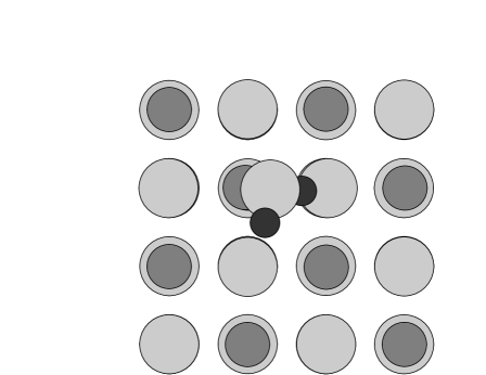
a) b)

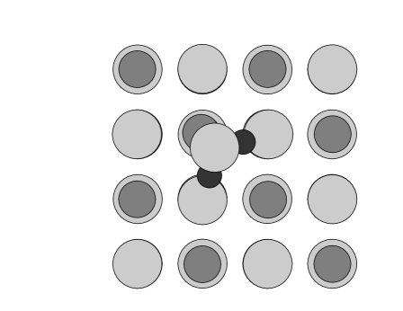
c) d)

Figure 1: Top and side views of the ‘tilted’ ( panels a, b) and ‘flat’ (panels c, d) configurations of the H₂O molecule adsorbed on the MgO (001) surface. Oxygen: large white spheres; Mg: medium grey spheres; H: small black spheres.

With PBE calculations, the most stable adsorbed configuration we have found (Fig. 1a,b) has the water O bound to a surface Mg, one of the two O-H bonds directed to a surface O, and the other tilted up at an angle to the surface plane. In this ‘tilted’ geometry, $E_{\rm ads}$ is converged to within $\sim 1$ meV with a slab containing three layers of ions and vacuum width of 12.7 Å (this is the distance between the layers of surface ions that face each other across the vacuum gap). With a $2\times 2$ surface unit cell (16 ions per layer in the repeating cell), $E_{\rm ads}$ is converged to better than 5 meV. With these settings, $\Gamma$-point sampling achieves convergence to within 5 meV. The static adsorption energy given by PBE in this geometry is 0.46 eV. The calculations also reveal a second stable adsorbed configuration having a slightly lower $E_{\rm ads}$ of 0.45 eV, in which the water O is bound, as before, to a surface Mg ion, but with the molecular plane almost flat on the surface, and with both O-H bonds directed to surface O ions (Fig. 1c,d). When the calculations are repeated with the LDA, we find that for the ‘flat’ adsorbed geometry $E_{\rm ads}$ is 0.95 eV. The large difference between the PBE and LDA values of $E_{\rm ads}$ indicates that quantitative agreement between theory and experiment cannot be expected without calibrating DFT calculations against more reliable methods.

Guided by these tests, we have performed all the following calculations with the 3-layer $2\times 2$ slab (48 ions in the MgO slab per repeating unit), a vacuum gap of 12.7 Å, and $\Gamma$-point sampling. Only the PBE approximation is used from now on. At all temperatures, we set the lattice parameter equal to $4.23$ Å, which is the $T=0$ K value in the bulk crystal, according to PBE.

3.2 Results for PMF, chemical potential and desorption rate

We have stressed that the feasibility of the present scheme depends on being able to make the statistical errors on $\langle{\cal F}_{z}\rangle_{z}$ small enough with simulation runs of affordable length. We use the analysis presented in Appendix A to determine the statistical errors on $\Delta\mu^{\dagger}$. We find that at $400$ K, with typically 15 $z$-points and with runs of 40 ps duration at each $z$-point, the statistical error on $\Delta\mu^{\dagger}$ is less than 20 meV, which is much better than the accuracy we are aiming for. The statistical errors are similar at other temperatures.

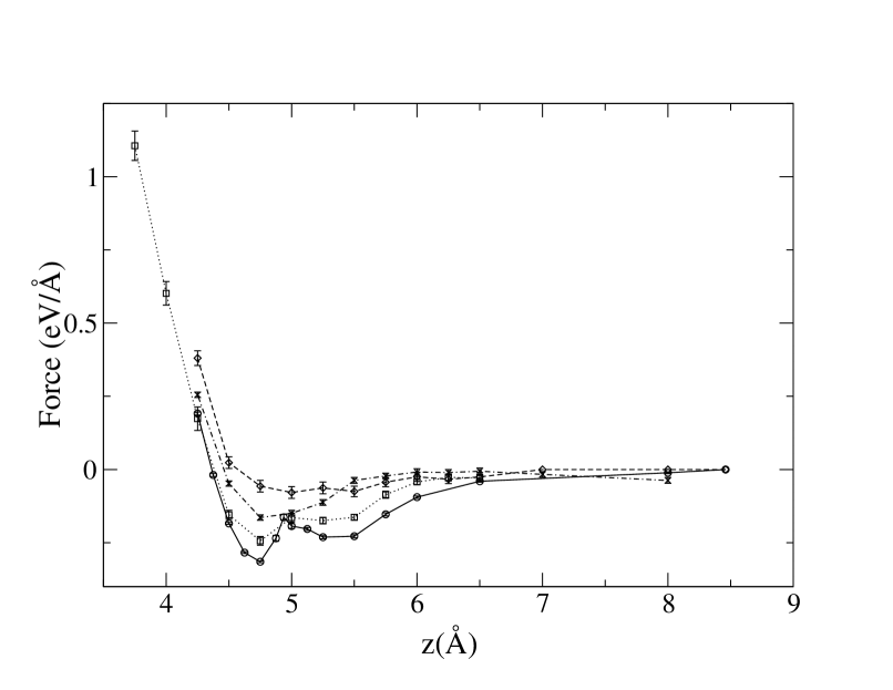
Figure 2: The mean force $\langle{\cal F}_{z}\rangle_{z}$ on the water O atom as function of its height $z$ above the surface at $T=100$, 300, 600 and 800 K (solid, dotted, chain and dashed curves, respectively, are guides to the eye). Bars on data points show statistical errors. Height $z$ is relative to a fixed atom in the centre of the slab.

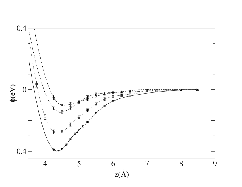
Figure 3: Potential of mean force $\phi(z)$ of the water O atom as function of its height $z$ above the surface at $T=100$, 300, 600 and 800 K. Symbols and curves have same meaning as in Fig. 2.

The mean force and the PMF from our simulations at four temperatures are reported in Figs. 2 and 3. We note the strong temperature dependence of both quantities. Interestingly, $\langle{\cal F}_{z}\rangle_{z}$ shows a double minimum at low $T$, which we believe is due to the fact that the characteristic orientation of the H₂O molecule changes substantially with $z$. The temperature dependence of the well-depth in $\phi(z)$ is closely related to the entropy part of $\Delta\mu^{\dagger}$, as can be seen by representing $\phi(z)$ in the simple form $\phi(z)=\phi_{\rm min}+\frac{1}{2}c(z-z_{\rm min})^{2}$, where $\phi_{\rm min}$ is the (negative) value of $\phi(z)$ and $c$ is the curvature at the bottom of the well. With this approximation, we have:

$$\Delta\mu^{\dagger}=k_{\rm B}T\ln\left[d^{-1}(2\pi k_{\rm B}T/c)^{1/2}\exp(-\beta\phi_{\rm min})\right]=-\phi_{\rm min}(T)+\frac{1}{2}k_{\rm B}T\ln(2\pi k_{\rm B}T/cd^{2})\;.$$ (14)

Then the entropy $s=-\partial\Delta\mu^{\dagger}/\partial T$ is:

$$s=-\frac{1}{2}k_{\rm B}\left(1+\ln(2\pi k_{\rm B}T/cd^{2})\right)+\partial\phi_{\rm min}/\partial T\;.$$ (15)

The first term on the right represents the entropy contribution from confinement of the $z$-coordinate of the molecule. The second term, which is positive (the well-depth decreases with increasing $T$), is due to the confinement of its translational and rotational degrees of freedom, as will be discussed in more detail below. Our calculated values of $\Delta\mu^{\dagger}$ at the four simulation temperatures vary rather linearly with $T$, and this implies that the isosteric heat of adsorption $h_{\rm iso}$ deviates only slightly from the $T=0$ K value of the adsorption energy $E_{\rm ads}$.

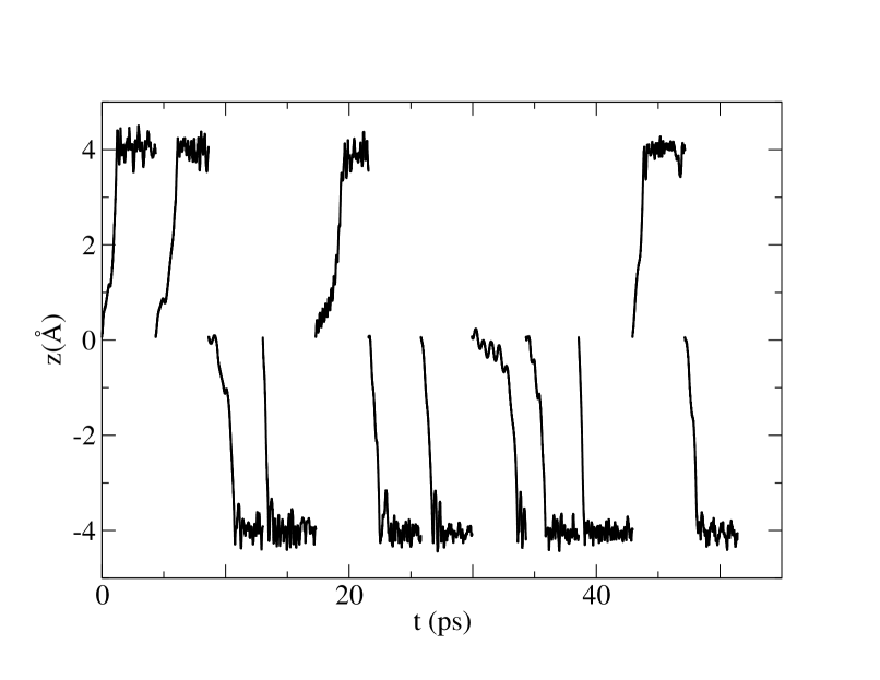
Figure 4: Set of 12 trajectories from simulations used to determine sticking coefficient $S$. Plots show $z$-coordinate (Å units) of water O atom relative to centre of vacuum gap between slabs.

In order to obtain the temperature-dependent desorption rate $\gamma$, we need to know the sticking coefficient $S$. We expect this to be close to unity, because the PMF shows that there is no barrier to adsorption. To test whether $S$ deviates significantly from zero, we have conducted a series of simulations in which the 3-layer MgO slab has already been well equilibrated at a given temperature $T$; the H₂O molecule is initially in the middle of the vacuum gap, and its atoms are given random velocities corresponding to that $T$. The subsequent time evolution is then monitored. We show in Fig. 4 the results of 12 such simulations at $T=400$ K. We see that in all cases H₂O becomes adsorbed on the surface, and there is no indication of desorption in the period of several ps after adsorption, during which time the molecule will have become well equilibrated on the surface. In the light of this, it is an accurate approximation to set $S=1$.

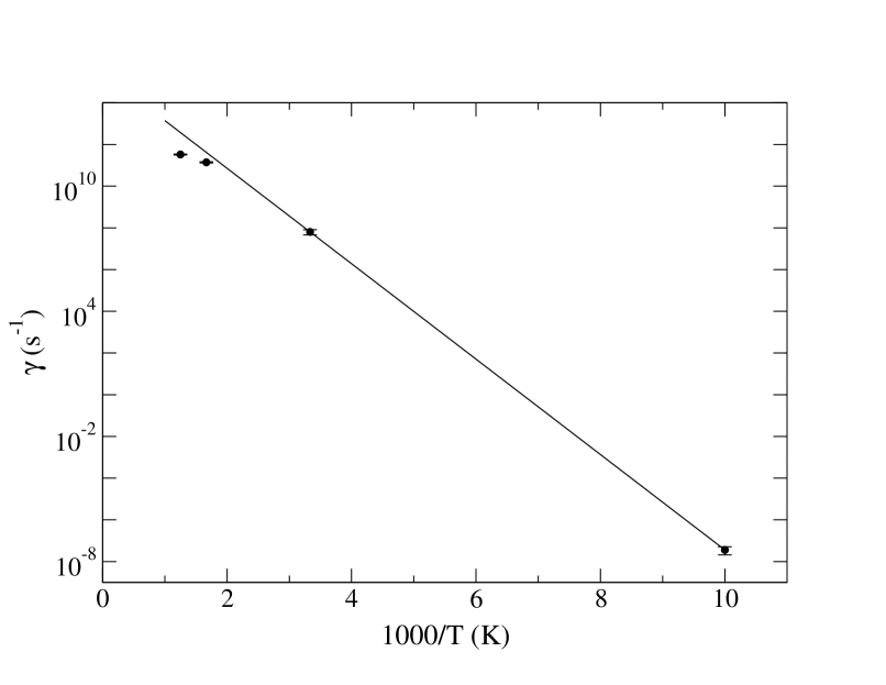
Figure 5: Arrhenius plot of the desorption rate $\gamma$ of H₂O from MgO (001) calculated using the PBE exchange-correlation functional. Bars on calculated values show statistical errors. The straight line is drawn to pass through the calculated values at the two lowest temperatures.

Numerical values of the desorption rate $\gamma$ as a function of $T$ calculated from eqn (12) are shown as an Arrhenius plot in Fig. 5. We have only a few data points, but the Arrhenius plot appears to rather straight, except at the highest $T$. This means that our results are fairly well described by the Polanyi-Wigner formula, eqn (1). We note that for the present case of low-coverage desorption in the absence of dissociation, the reaction order $n$ is unity, so that the Polanyi-Wigner formula becomes $\gamma=-\theta^{-1}d\theta/dt=f\exp(-\Delta E/k_{\rm B}T)$. If we pass a straight line through the points at the two lowest temperatures in fig. 5, we obtain an activation energy $\Delta E=0.454$ eV, and a prefactor $f=2.7\times 10^{15}$ s^-1. We note that the activation energy is almost exactly equal to the zero-temperature static adsorption energy $E_{\rm ads}=0.46$ eV. In the temperature range $200-300$ K, where thermal desorption of H₂O from MgO (001) is experimentally observed at sub-monolayer coverage, the calculated prefactor of $2.7\times 10^{15}$ s^-1 is thus enhanced by a factor of $\sim 270$ above the value of $10^{13}$ s^-1 often used in analysing TPD measurements on this system in the past [28, 29].

The enhancement of the prefactor arises from the $T$-dependence of the PMF. On substituting the approximate form of $\Delta\mu^{\dagger}$ given by eqn (14) into eqn (12), we find:

$$\gamma=S\left(c\left/4\pi^{2}M_{\rm A}\right.\right)^{1/2}\exp(\beta\phi_{\rm min})\;.$$ (16)

The factor $(c/4\pi^{2}M_{\rm A})^{1/2}$ is the oscillation frequency of the centre of mass of the molecule along the surface normal. If $\phi_{\rm min}$ varies roughly linearly with $T$, then $\phi_{\rm min}=-E_{\rm ads}+T(\partial\phi_{\rm min}/\partial T)$, so that $\gamma=S(c/4\pi^{2}M_{\rm A})^{1/2}\exp(k_{\rm B}^{-1}\partial\phi_{\rm min}/\partial T)\exp(-\beta E_{\rm ads})$. The enhancement factor is thus $\exp(k_{\rm B}^{-1}\partial\phi_{\rm min}/\partial T)$, and it comes from the part of the adsorption entropy associated with confinement of the translational and rotational degrees of freedom other than oscillation along the surface normal.

3.3 Spatial distribution and memory

We now discuss two important questions. The first concerns the more detailed interpretation of the prefactor enhancement. Since this is due to confinement of degrees of freedom of the molecule, it should be possible to relate it to the probability distributions of these degrees of freedom. The second question concerns the crucial assumption underlying our calculation of the desorption rate, that equilibration rates of the adsorbed molecule are faster than the desorption rate. Equilibration rates are related to memory times, and we want to use our simulations to characterise these memory times.

Since H₂O contains three atoms, it has nine degrees of freedom. One of these is bodily vibration along the surface normal, whose distribution is $y(z)$. The three internal vibrational modes of the molecule do not undergo large changes on adsorption at low coverage, so that they do not contribute significantly to the enhancement of $f$. The enhancement therefore comes from the remaining degrees of freedom, two of which refer to translation in the surface plane, and the other three to rotations. We describe in Appendix B how the enhancement factor can be related semi-quantitively to the non-uniformity of the probability distributions of these degrees of freedom.

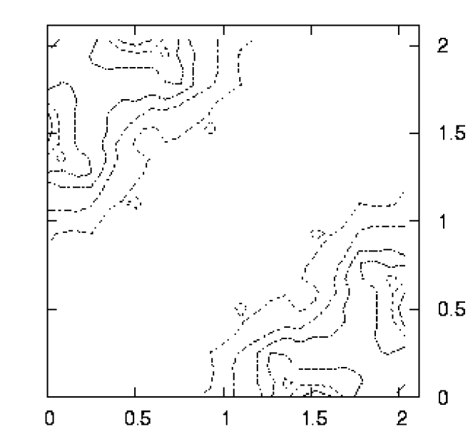
Figure 6: Contour plot of the spatial probability distribution of water O atom in the $x$-$y$ plane at $T=400$ K. Bottom right and top left corners of plot are Mg sites; bottom left and top right corners are O sites. Probability density is in arbitary units, with equal spacing between contours.

We examine the reduced freedom of the translational motion by plotting the probability distribution $p_{\rm tr}(x,y)$ of the $x$- and $y$-coordinates of the water O atom. This is done by dividing the surface plane into a square grid, and accumulating the frequencies with which $x$ and $y$ fall in each cell of the grid. Since $p_{\rm tr}(x,y)$ has the translational symmetry of the crystal surface, we can improve the statistics by averaging over symmetry related cells. From our calculated $p_{\rm tr}(x,y)$ at $T=400$ (Fig. 6), we see that the water O spends most of its time close to surface Mg sites, in line with our finding (Sec. 3.1) that the most stable relaxed configuration of H₂O on the surface has water O coordinated to surface Mg. However, it is also clear that the most probable O position is not directly above Mg, but is displaced to positions roughly along a cubic axis in the surface plane. This agrees with our static calculations on the tilted configuration.. The analysis of Appendix B shows that we can estimate the entropy reduction associated with $p_{\rm tr}(x,y)$ as follows. We fit the calculated $p_{\rm tr}(x,y)$ with a superposition of four Gaussians $A\exp\left(-\alpha|{\bf r}-{\bf R}|^{2}\right)$, centred at the positions $\delta x(\pm 1,0)$ and $\delta x(0,\pm 1)$ relative to the Mg site, using $\alpha$ and $\delta x$ as fitting parameters. We then normalise the resulting smoothed distribution so that $\int_{\rm cell}dx\,dy\,p_{\rm tr}(x,y)=1$ where the integral goes over the surface unit cell, whose area is $A_{\rm cell}$. Denoting by $c_{1}$ the constant such that the maximum value of $c_{1}p_{\rm tr}(x,y)$ in the cell is unity, the contribution to the enhancement factor from translational confinement is estimated as $b_{1}=A_{\rm cell}/c_{1}$. At $T=300$ and 400 K, we find $b_{1}=3.8$ and 2.9, respectively.

The orientation of the molecule is specified by three angles $\theta$, $\phi$ and $\psi$. These characterise the orientation of the molecule relative to a reference orientation, which we choose to be such that the bisector of the H-O-H bond points along the outward normal, with the plane of the molecule lying in the $x$-$z$ plane (the $x$-axis is along one of the cubic axes of the substrate). From this starting point, we can produce any other orientation in three steps: (i) rotate the molecule about the bisector by angle $\phi$; (ii) rotate the molecule by angle $\theta$ about the axis perpendicular to the bisector in the molecular plane (the result of this is that the bisector makes an angle $\theta$ with the surface normal); (iii) rotate the molecule about the bisector by angle $\psi$. The angles $(\theta,\phi,\psi)$ are thus the conventional Euler angles specifying rigid-body rotation of the molecule.

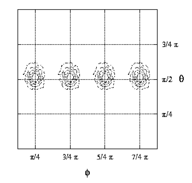
Figure 7: Contour plot of probability distribution of angles $\theta$ and $\phi$ specifying orientiation of the bisector of H₂O molecule (see text) at $T=400$ K. Peaks of the distribution correspond to the four equivalent orientations in which the bisector is nearly parallel to the surface ($\theta\simeq\frac{1}{2}\pi$), and points along one of the diagonal directions ($\phi=\frac{1}{4}\pi$, $\frac{3}{4}\pi$, $\frac{5}{4}\pi$, and $\frac{7}{4}\pi$).

The probability distribution $p_{\rm bis}(\theta,\phi)$ of the bisector is computed by dividing the $\theta$ range $(0,\pi)$ and the $\phi$ range $(0,2\pi)$ into a uniform grid and accumulating a two-dimensional histogram. The contour plot of $p_{\rm bis}(\theta,\phi)$ at $T=400$ K (Fig. 7) shows that the direction of the bisector is always quite close to the surface plane, and within this plane tends to point along one of the diagonal directions. (This is exactly the orientation of the ‘flat’ configuration (Fig. 1), in which the two O-H bonds are directed from a surface Mg site to two of the nearest-neighbour O sites.) This being so, the angle $\psi$ effectively measures the tilt of the molecular plane relative to the surface. The rather broad calculated probability distribution $p_{\rm sp}(\psi)$ of the angle $\psi$ (Fig. 8), centred on $\psi=0$, means that the molecular plane tilts relative to the surface over a rather wide range. The double-peaked structure of the distribution indicates that the untilted configuration is not the most stable, again in accord with our static results.

The reduction of rotational freedom associated with $(\theta,\phi)$ is estimated by fitting the distribution $p_{\rm bis}(\theta,\phi)$ to a superposition of Gaussians. As explained in Appendix B, the contribution $b_{2}$ to the enhancement factor due to confinement of $\theta$ and $\phi$ is estimated by a procedure similar to the one used for translational confinement. At $T=300$ and 400 K, we find $b_{2}=19.9$ and 16.0, respectively. Finally, analysing the confinement of $\psi$ shown in Fig. 8, we obtain enhancement contribution $b_{3}=2.8$ and 2.4 at $T=300$ and 400 K, respectively. Combining all the translational and rotational factors, we arrive at total enhancement factor of 212 and 111 at $T=300$ and 400 K, which are roughly consistent with what we obtained from our numerical results for $\gamma$.

Turning now to the question of memory times, we want to give evidence about the dynamics of the two processes that are likely to have the longest memory times, namely hopping between different surface sites, and transitions between different orientations. We have attempted to calculate appropriate correlation functions, but with only a single molecule in the system, it is not possible yet to achieve good statistics. The data we present are therefore only semi-quantitative.

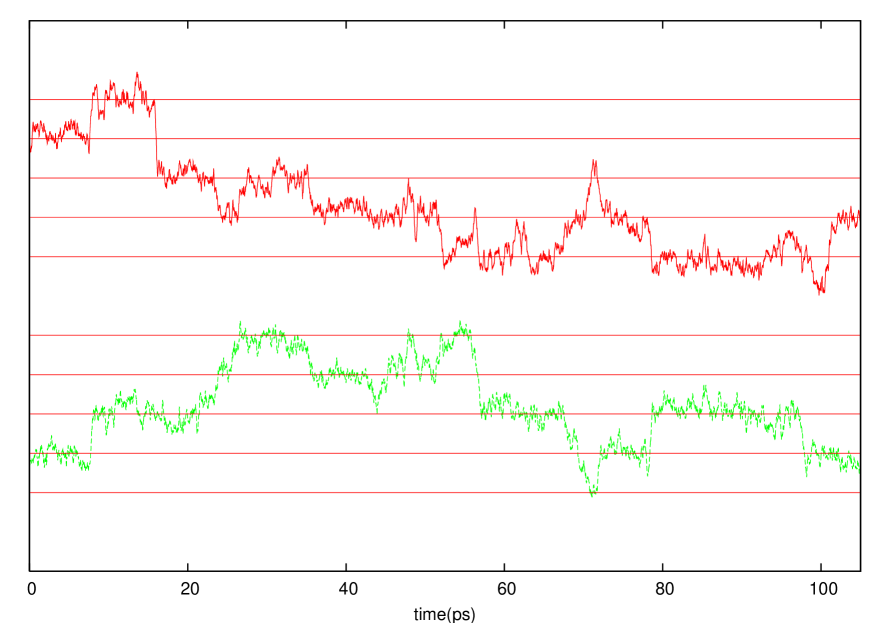
Figure 9: Time variation of the $x$- and $y$-coordinates of the water O atom in the course of an m.d. simulation at $T=400$ K. Horizontal lines mark $x$- and $y$-coordinates of perfect-lattice sites, so that spacing between neighbouring lines is $\frac{1}{2}a_{0}=2.115$ Å.

To illustrate the translational dynamics, we show in Fig. 9 the time-dependent $x(t)$ and $y(t)$ coordinates of the water O over the 100 ps span of an unconstrained simulation at 400 K. We see several well-defined intersite jumps in which $x$ and/or $y$ change by the Mg-O nearest-neighbour distance $d=2.12$ Å. In most of these jumps, both $x$ and $y$ change, and this indicates a diagonal jump between Mg sites, but there are events in which one coordinate changes by $2d$, with no change in the other. By simple counting of jumps, we estimate a hopping rate of $1.4\times 10^{11}$ s^-1. The same procedure at $T=300$ K gives a hopping rate of $3.8\times 10^{10}$ s^-1. To interprete these results further, we have made nudged elastic band calculations [30] of the energy barrier for intersite hopping, and we find the value 0.13 eV. This is roughly consistent with the ratio of hopping rates of about 3.7 between 300 and 400 K. It is clear from this that, in this temperature region, intersite hopping is very much more rapid than the desorption rate, and this will become even more true at lower temperatures.

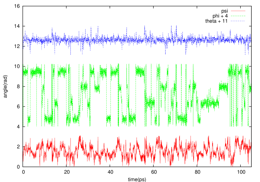
Figure 10: Time variation of the angles $\theta$ (top), $\phi$ (middle) and $\psi$ (bottom) specifying orientation of the molecule (see text) during the course of an m.d. simulation at 400 K.

To display the rotational dynamics, we show in Fig. 10 plots of the angles $\theta(t)$, $\phi(t)$ and $\psi(t)$ during the course of the simulation at 400 K. The dynamics of $\theta$ and $\psi$ consists of very rapid fluctuations on a time scale of 1 ps or less, over the range expected from the probability distributions of Figs. 7 and 8. The angle $\phi$ has somewhat slower dynamics associated with hopping between the four equivalent sub-sites around each Mg site (Figs 1 and 7), but at $T=400$ K, this hopping rate is $\sim 5\times 10^{11}$ s^-1, which is several times faster than the hopping rate between sites.

The conclusion from this is that all equilibration rates on the surface appear to be very much faster than the desorption rate at temperatures of interest.

4 Discussion

The practical calculations we have presented show the feasibility of calculating thermodynamic properties of a surface adsorbate by ab initio methods, without recourse to a lattice-gas approximation. We have assumed nothing at all about the adsorption sites of H₂O on MgO (001), and the ab initio m.d. simulations themselves automatically sample the sites and orientiations that are statistically significant. In the same spirit, we completely avoid approximations such as the harmonic approximation, and we fully include the coupling of the molecular and substrate degrees of freedom. In this sense, there are no statistical-mechanical approximations whatever, except for the neglect of quantum nuclear effects, to which we return below. The single uncontrollable approximation is the DFT exchange-correlation functional. Furthermore, when calculating the desorption rate, we do not assume the validity of the Polanyi-Wigner formula, but we use this formula only as a means of fitting the computed results. In this way, we obtain an ab initio value of the frequency prefactor.

It is well known from both experiments [31] and simulations [19] on a wide range of systems that frequency prefactors for thermal desorption often differ, sometimes by many orders of magnitude, from the value of $10^{13}$ s^-1 that might naively be expected if the prefactor is thought of as an “attempt frequency”. It is also well known that this is due to the strong reduction of translational, rotational and conformational entropy that often occurs when a molecule goes from the gas phase to the adsorbed state. For H₂O on MgO (001), our calculated prefactor has the value $f=2.7\times 10^{15}$ s^-1, so that it is enhanced by a factor of over $100$ above the typical vibrational frequency of the molecule relative to the surface. We have seen that an enhancement factor of this general size is expected from the translational and rotational probability distribution functions of the molecule.

A crucial assumption behind the Polanyi-Wigner formula is that the desorption rate depends only on the instantaneous temperature and coverage, and is not history dependent. A key condition for this to be true is that the equilibration rate of the molecule on the surface be faster than the desorption rate. We have attempted to characterise the typical equilibration times for the isolated H₂O molecule on MgO (001) by studying the diffusional and rotational dynamics, and we have found that the condition is satisfied by a margin of several orders of magnitude in the temperature region where thermal desorption can be experimentally observed.

A direct comparison with experimental TPD data for H₂O on MgO (001) is not straightforward. There have been several TPD studies reported [28, 29], some of which refer to carefully prepared surfaces that appear to be relatively free of defects. Desorption at sub-monolayer coverage is associated with a TPD peak at $\sim 245$ K. In our simulated system, the desorption rate at this $T$ is $\sim 2.6\times 10^{6}$ s^-1, so that all molecules would desorb in less than 10 $\mu$s, which is many orders of magnitude less than the time-scale of a TPD experiment. This might suggest that the adsorption energy of 0.46 eV given by the PBE functional we have used is considerably too low. However, the effect of attractive water-water interactions may be important even at coverages well below the monolayer level. In fact, adsorption isotherm measurements indicate a critical point in the surface phase diagram of H₂O on MgO (001) at $T\simeq 210$ K [32]. The effect of water-water interactions on the desorption rate clearly needs to be quantified. A further complication is that we have so far ignored quantum nuclear effects. Because of the very high vibrational frequencies of the water molecule, it is possible that changes of zero-point energy on adsorption might shift $E_{\rm ads}$ significantly. Even without all these effects, it is not clear that we should expect good agreement with experiment yet, because the calculated $E_{\rm ads}$ depends so much on the exchange-correlation functional. The frequency prefactor $f$ might also depend significantly on exchange-correlation functional. If we assume provisionally that our calculated $f$ of $2.7\times 10^{15}$ s^-1 is essentially correct, and we ignore water-water interactions, then the experimental TPD peak temperature of 245 K would require an activation energy $\Delta E=0.78$ eV, which is well above the PBE adsorption energy of 0.46 eV, though it is still below the LDA value of 0.95 eV. It is clear that DFT predictions of $E_{\rm ads}$ need to be tested against more accurate and reliable methods.

A number of future challenges are suggested by this work. The most obvious of these is the extension of the calculations to higher coverages. According to the theory we have presented, the calculation of the PMF on a chosen molecule, and the integration of the resulting distribution function $y(z)$, allows us to calculate the chemical potential and the desorption rate at arbitrary temperature and coverage. At the time of writing, we have performed exploratory ab initio calculations of this kind for H₂O on MgO (001) at coverages of 0.25 and 0.5 ML. However, the problem that emerges is that the memory times are much longer than for the isolated molecule, so that considerably longer simulations are needed in order to achieve acceptable statistical accuracy. This problem of statistical sampling becomes rapidly worse at low temperatures, and so far we have achieved stastically accurate results only at $T=800$ K, which is well above the region of practical interest. A second important challenge is that of going beyond DFT. We have noted that the LDA and GGA forms of exchange-correlation functional give static adsorption energies differing by roughly a factor of two. This means that we must envisage future calculations of the present kind, but performed by post-DFT techniques. The recent proposal of a method for performing quantum Monte Carlo simulations along an m.d. trajectory [33] may indicate one way to do this. Recent successes in applying high-level quantum chemistry to condensed-matter energetics are also promising [34]. A third challenge is that of eliminating the approximation of classical statistical mechanics for the nuclei. For the case of H₂O on MgO (001), the errors due to the use of the classical approximation will not be large, but may be significant if one wishes to achieve chemical accuracy. We will report in the second paper of this series on the generalisation of the present theory to quantum statistical mechanics for the nuclei, using path-integral ab initio simulation.

5 Conclusions

In summary, we have shown how ab initio methods can be used to calculate the chemical potential of an adsorbate, with full inclusion of entropy effects. The methods used can in principle be applied at any coverage. We have shown how the methods also yield values for the desorption rate and hence the frequency pre-factor in the Polanyi-Wigner formula. For the case of H₂O on MgO (001) at low coverage, this pre-factor is enhanced by at least two orders of magnitude above the values generally assumed in the past, and we have given a detailed interpretation of this enhancement in terms of the confinement of translational and rotational degrees of freedom. The crucial condition of rapid equilibration necessary for the validity of the Polanyi-Wigner formula appears to be satisfied by a wide margin for low-coverage H₂O on MgO (001). Preliminary comparisons with experimental data suggest that for this system the adsorption energy given by PBE may significantly too low.

Appendix A: Analysis of statistical errors

We explained in Secs. 2.3 and 3.2 the importance of monitoring the statistical errors in the calculation of the mean force $\langle{\cal F}_{z}\rangle_{z}$ and hence of the PMF and the chemical potential. We summarise here how we have estimated the errors on the mean force, and how we have used this to estimate the errors on the other quantities.

The mean force is calculated at a set of $z$-values: $z_{0}>z_{1},\ldots>z_{n}$. At a given $z$-value $z_{i}$, the estimate ${\cal F}_{i}$ of the mean force obtained by averaging over the length of the run differs from the exact value ${\cal F}_{i}^{\rm ex}$ that would be obtained if the sampling were perfect. We denote by $\delta{\cal F}_{i}\equiv{\cal F}_{i}-{\cal F}_{i}^{\rm ex}$ the difference that occurs in a given simulation run. We estimate the standard deviation $\langle\delta{\cal F}_{i}^{2}\rangle^{1/2}$ by the usual re-blocking method. In this method the simulation of total duration $\tau$ is divided into $\nu$ blocks, each of duration $\tau/\nu$, and we compute an estimate ${\cal F}_{i}(l)$ of ${\cal F}_{i}$ for each block $l$. Then, we compute the quantity $\sigma_{\nu}^{2}=\nu^{-1}\sum_{l=1}^{\nu}\left({\cal F}_{i}(l)-\bar{\cal F}_{i}\right)^{2}$, where $\bar{\cal F}_{i}$ is the estimate obtained by averaging over the entire time $\tau$. If the duration $\tau/\nu$ of each block is short, the block averages $\bar{\cal F}(l)$ are strongly correlated, and $\sigma_{\nu}$ underestimates the true statistical error. However, as the duration of the blocks becomes longer than the correlation time, the ${\cal F}_{i}(l)$ become statistically independent, and $\sigma_{\nu}$ tends to a plateau value. The reblocking technique consists of plotting $\sigma_{\nu}$ against $\tau/\nu$ and taking the standard deviation $\langle\delta{\cal F}_{i}^{2}\rangle^{1/2}$ to be the plateau value of $\sigma_{\nu}$ as $\nu$ is decreased.

We now turn to the statistical error on the PMF, denoting the value of $\phi(z)$ at the $i$th $z$-point obtained from a given set of simulation runs by $\phi_{i}$, the exact value by $\phi_{i}^{\rm ex}$ and the difference $\phi_{i}-\phi_{i}^{\rm ex}$ by $\delta\phi_{i}$. Since the $\phi_{i}$ values are obtained by integrating inward from the largest $z$-value $z_{0}$ using the trapezoidal rule, we have:

$$\phi_{i} = \phi_{0}+\frac{1}{2}\sum_{n=1}^{i}(z_{j-1}-z_{j})({\cal F}_{j}+{\cal F}_{j-1})$$ (17)

$$= \phi_{0}+\frac{1}{2}(z_{0}-z_{1}){\cal F}_{0}+\frac{1}{2}\sum_{j=1}^{i-1}(z_{j-1}-z_{j+1}){\cal F}_{j}+\frac{1}{2}(z_{i-1}-z_{i}){\cal F}_{i}\;.$$

The errors on ${\cal F}_{j}$ and ${\cal F}_{k}$ are statistically independent for $j\neq k$, so that:

$$\langle\delta\phi_{i}^{2}\rangle=\langle\delta\phi_{0}^{2}\rangle+\frac{1}{4}\left[(z_{0}-z_{1})^{2}\langle\delta{\cal F}_{0}^{2}\rangle+\sum_{j=1}^{i-1}(z_{j-1}-z_{j+1})^{2}\langle\delta{\cal F}_{j}^{2}\rangle+(z_{i-1}-z_{i})^{2}\langle\delta{\cal F}_{i}^{2}\rangle\right]\;.$$ (18)

Now to estimate the statistical error on $\Delta\mu^{\dagger}$, we recall (eqn (11)) that $\Delta\mu^{\dagger}=k_{\rm B}T\ln Y$, where $Y=d^{-1}\int_{-\infty}^{z_{0}}dz\,\exp(-\beta\phi(z))$. In practice, the integral comes almost entirely from a narrow region of $z$ around the value $z_{\rm min}$ where $\phi(z)$ has its minimum. But the statistical fluctuations of $\phi_{i}$ at $z_{i}$ that are near each are almost perfectly correlated, since the fluctuation $\delta\phi_{i}$ comes from the accumulation of fluctuations $\delta{\cal F}_{j}$ at many points $z_{j}>z_{i}$. So to calculate the fluctuation of $Y$, it is a good approximation to say that the fluctuations of all $\phi_{i}$ in the region of $z_{\rm min}$ are perfectly correlated. This means that $\delta Y=-\beta\delta\phi_{\rm min}Y$, where $\delta\phi_{\rm min}$ is the fluctuation of $\delta\phi_{i}$ for $z_{i}\simeq z_{\rm min}$. Then since $\delta\Delta\mu^{\dagger}=k_{\rm B}T\delta Y/Y$, we finally obtain the estimate for the standard deviation $\langle\left(\delta\Delta\mu^{\dagger}\right)^{2}\rangle^{1/2}=\langle\delta\phi_{\rm min}^{2}\rangle^{1/2}$, with $\langle\delta\phi_{\rm min}^{2}\rangle^{1/2}$ calculated according to eqn (18).

Appendix B: Translational and rotational distributions and enhancement of the frequency prefactor

We noted in the text that the entropy of the adsorbed molecule is less than that of the free molecule, because its translational and rotational freedom is reduced. This entropy reduction is closely related to the enhancement of the frequency prefactor $f$ above its naively expected value of $\sim 10^{13}$ s^-1. We want to make a semi-quantitative connection between the entropy reduction and the translational and rotational distributions presented in Sec. 3.3.

For this interpretative purpose, we ignore the degrees of freedom of the substrate, and we assume that the $x$-$y$ translational distribution, the $z$-distribution, the $\theta$-$\phi$ distribution and the $\psi$ distribution are all independent of each other. This is equivalent to supposing that the distribution over $x$, $y$, $z$, $\theta$, $\phi$ and $\psi$ is governed by a Boltzmann factor $\exp(-\beta V(x,y,z,\theta,\phi,\psi))$, where $V$ is expressed as:

$$V(x,y,z,\theta,\phi,\psi)=-V_{0}+\frac{1}{2}\alpha z^{2}+u(x,y)+v(\theta,\phi)+w(\psi)\;.$$ (19)

Here, $-V_{0}$ represents the energy of the molecule in its most stable adsorbed configuration, which implies that $u\geq 0$, $v\geq 0$ and $w\geq 0$. Then the distribution $y(z)$ defined in Sec. 2.1 is given by:

$$y(z)=C\exp\left[-\beta\left(-V_{0}+\frac{1}{2}\alpha z^{2}\right)\right]$$ (21)

$$\times\int_{\rm cell}dx\,dy\,e^{-\beta u(x,y)}\;\int_{0}^{2\pi}d\phi\,\int_{0}^{\pi}d\theta\,\sin\theta e^{-\beta v(\theta,\phi)}\;\int_{0}^{2\pi}d\psi\,e^{-\beta w(\psi)}$$

for $z$ near the surface, where the $x$-$y$ integration goes over a single surface unit cell. By definition, $y(z)=1$ far from the surface, and this fixes the constant $C$:

$$1=8\pi^{2}CA_{\rm cell}\;,$$ (22)

where $A_{\rm cell}$ is the area of the surface unit cell. In this approximation, the factor $B$ by which the frequency prefactor is enhanced is the product of three factors: $B=b_{1}b_{2}b_{3}$, where:

$$b_{1} = A_{\rm cell}\left/\int_{\rm cell}dx\,dy\,e^{-\beta u(x,y)}\right.$$

$$b_{2} = 4\pi\left/\int_{0}^{2\pi}d\phi\int_{0}^{\pi}d\theta\,\sin\theta e^{-\beta v(\theta,\phi)}\right.$$

$$b_{3} = 2\pi\left/\int_{0}^{2\pi}d\psi\,e^{-\beta w(\psi)}\right.\;.$$ (23)

The potential of mean force $\phi(z)$, defined by $y(z)=\exp(-\beta\phi(z))$, is then given by:

$$\phi(z)=-V_{0}+\frac{1}{2}\alpha z^{2}+k_{\rm B}T\ln(b_{1}b_{2}b_{3})\;,$$ (24)

so that the value of $z$ at the minimum of $\phi$ and the curvature at the minimum remain the same, but the well becomes less deep with increasing temperature, because of the factor $k_{\rm B}T\ln(b_{1}b_{2}b_{3})$.

We estimate the values of the factors $b_{i}$ from the probability distributions as follows. We calculate the probability distribution $p_{\rm tr}(x,y)$ by histogram accumulation, as described in Sec. 3.3, and normalise it so that $\int_{\rm cell}dx\,dy\,p_{\rm tr}(x,y)=1$. We then determine the constant $c_{1}$ such that the maximum value of $c_{1}p_{\rm tr}(x,y)$ in the cell is unity ($c_{1}$ thus has dimensions of area). We then have $b_{1}=A_{\rm cell}/c_{1}$. Similarly, with probability distribution $p_{\rm bis}(\theta,\phi)$ normalised so that $\int d\phi\,d\theta\,\sin\theta\,p_{\rm bis}(\theta,\phi)=1$, we find the constant $c_{2}$ such that the maximum value of $c_{2}p_{\rm bis}(\theta,\phi)$ is unity. Then $b_{2}=4\pi/c_{2}$. Similarly for $b_{3}$.

Figure 8: Contour plot of probability distribution of angle $\psi$ specifying rotation of H₂O molecule about its bisector (see text) at $T=400$ K. When the molecular bisector is parallel to the surface, the molecular plane is parallel to the surface when $\psi=\frac{1}{2}\pi$.

References

- [1] K. Reuter and M. Scheffler, Phys. Rev. Lett., 90, 046103 (2003).
- [2] K. Honkala, A. Hellman, I. N. Remediakis, A. Logadottir, A. Carlsson, S. Dahl, C. H. Christensen and J. K. Norskov, Science, 307, 555 (2005).
- [3] D. Alfè and M. J. Gillan, J. Phys. Condens. Matter, 18, L451 (2006).
- [4] E. Smargiassi and P. A. Madden, Phys. Rev. B, 51, 117 (1995).
- [5] O. Sugino and R. Car, Phys. Rev. Lett., 74, 1823 (1995).
- [6] G. de Wijs, G. Kresse and M. J. Gillan, Phys. Rev. B, 57, 8223 (1998).
- [7] D. Alfè, M. J. Gillan and G. D. Price, Nature, 401, 462 (1999).
- [8] M. J. Gillan, D. Alfè, J. Brodholt, L. Vočadlo and G. D. Price, Rep. Prog. Phys., 69, 2365 (2006).
- [9] C. Stampfl, H. J. Kreuzer, S. H. Payne, H. Pfnur and M. Scheffler, Phys. Rev. Lett., 83, 2993 (1999).
- [10] D. Alfè, G. D. Price and M. J. Gillan, Phys. Rev. B, 64, 045123 (2001).
- [11] D. Alfè, G. D. Price and M. J. Gillan, Phys. Rev. B, 65, 165118 (2002).
- [12] See e.g. R. I. Masel, Principles of Adsorption and Reaction on Solid Surfaces, Ch. 4, Wiley (1996).
- [13] W. M. C. Foulkes, L. Mitaš, R. J. Needs and G. Rajagopal, Rev. Mod. Phys., 73, 33 (2001).
- [14] M. Polanyi, Trans. Faraday Soc., 28, 314 (1932).
- [15] P. A. Redhead, Vacuum, 12, 203 (1962).
- [16] D. A. King, Surf. Sci., 47, 384 (1975).
- [17] M. Sprik and G. Ciccotti, J. Chem. Phys., 109, 7737 (1998) and references therein.
- [18] G. N. Patey and J. P. Valleau, J. Chem. Phys., 63, 2334 (1975);
- [19] K. A. Fichthorn and R. A. Miron, Phys. Rev. Lett., 89, 196103 (2002); K. E. Becker and K. A. Fichthorn, J. Chem. Phys., 125, 184706 (2006).
- [20] See e.g. A. Zangwill, Physics at Surfaces, Ch. 14, Cambridge University Press (1988).
- [21] S. Nosé, Mol. Phys., 52, 255 (1984); S. Nosé, J. Chem. Phys., 81, 511 (1984).
- [22] H. C. Andersen, J. Chem. Phys., 72, 2384 (1980).
- [23] P. Blöchl, Phys. Rev. B, 50, 17953 (1994).
- [24] G. Kresse and D. Joubert, Phys. Rev. B, 59, 1758 (1999).
- [25] G. Kresse and J. Furthmüller, Phys. Rev. B, 54, 11169 (1996).
- [26] See e.g. W. Langel and M. Parrinello, J. Chem. Phys., 103, 3240 (1995); K. Refson, R. A. Wogelius, D. G. Fraser, M. C. Payne, M. H. Lee and V. Milman, Phys. Rev. B, 52, 10823 (1995); L. Giordano, J. Goniakowski and J. Suzanne, Phys. Rev. Lett., 81, 1271 (2000); M. Odelius, Phys. Rev. Lett., 82, 3919 (1999); L. Giordano, J. Goniakowski and J. Suzanne, Phys. Rev. B, 62, 15406 (2000); L. Delle Site, A. Alavi and R. Lynden-Bell, J. Chem. Phys., 113, 3344 (2000); R. M. Lynden-Bell, L. Delle Site and A. Alavi, Surf. Sci., 496, L1 (2002).
- [27] J. P. Perdew, K. Burke and M. Ernzerhof, Phys. Rev. Lett., 77, 3865 (1996).
- [28] M. J. Stirniman, C. Huang, R. S. Smith, S. A. Joyce and B. D. Kay, J. Chem. Phys., 105, 1295 (1996).
- [29] C. Xu and W. Goodman, Chem. Phys. Lett., 265, 341 (1997).
- [30] G. Henkelman and H. Jonsson, J. Chem. Phys., 113, 9978 (2000).
- [31] K. R. Paserba and A. J. Gellman, Phys. Rev. Lett., 86, 4338 (2001); S. L. Tait, Z. Dohnálek, C. T. Campbell and B. D. Kay, J. Chem. Phys., 122, 164707; ibid. 122, 164708 (2005).
- [32] D. Ferry, A. Glebov, V. Senz, J. Suzanne, J. P. Toenies and H. Weiss, J. Chem. Phys., 105, 1697 (1996).
- [33] J. C. Grossman and L. Mitaš, Phys. Rev. Lett., 94, 056403 (2005).
- [34] F. R. Manby, D. Alfè and M. J. Gillan, Phys. Chem. Chem. Phys., 8, 5178 (2006).
a)
b)
b)
c)
d)
d)