Quantum Field Theoretical Analysis on Unstable Behavior of Bose-Einstein Condensates in Optical Lattices

Abstract

We study the dynamics of Bose-Einstein condensates flowing in optical lattices on the basis of quantum field theory. For such a system, a Bose-Einstein condensate shows a unstable behavior which is called the dynamical instability. The unstable system is characterized by the appearance of modes with complex eigenvalues. Expanding the field operator in terms of excitation modes including complex ones, we attempt to diagonalize the unperturbative Hamiltonian and to find its eigenstates. It turns out that although the unperturbed Hamiltonian is not diagonalizable in the conventional bosonic representation the appropriate choice of physical states leads to a consistent formulation. Then we analyze the dynamics of the system in the regime of the linear response theory. Its numerical results are consitent with as those given by the discrete nonlinear Schrödinger equation.

I Introduction

The Bose-Einstein condensates (BECs) of trapped atoms, first realized in 1995 Cornell ; Cornell2 ; Ketterle2 , are ideal systems for studying quantum many-body phenomena. This is because the systems are dilute, weakly interacting ones and we can easily control the configuration of the trap and even the strength of atomic interaction. Recently much attention has been focused on the BEC in an optical lattice, which provides us with rich phenomena such as superfluid-insulator quantum phase transition Greiner and Bloch oscillations Bloch , and also enables us to observe directly the quantum fluctuation as quantum depletion from the condensate depletion .

Fluctuations and excitation spectra of a BEC are determined from the Bogoliubov-de Gennes (BdG) equation, which is obtained by the linearization of the time dependent Gross-Pitaevskii (TDGP) equation. Numerical calculation of the excitation spectra of a BEC in an optical lattice was performed in Ref. Ichioka . The analytical studies under the tight-binding approximation Oosten ; Clark gave the theoretical result in a good agreement with the experiment depletion .

In this paper, we focus on the BECs flowing in optical lattices. For such a system, two types of instability are known: Landau and dynamical instabilities. The Landau instability is an energetic instability which is caused by negative energies of the quasi-particle Iigaya . The dynamical instability is that of condensates caused by the complex eigenvalues of the BdG equations Wu1 ; Wu2 . The Landau instability (energetic instability) is not observed at low temperature instaove2 , because it requires the thermal cloud which brings a dissipative mechanism and drives the condensate toward a lower energy state. On the other hand, the dynamical instability can occur even at zero temperature.

The emergence of complex eigenvalues in the BdG equations is not restricted to the superfluidity of BECs in optical lattices, but is found widely, such as in the BECs with highly quantized vortices Pu ; Garay ; Skryabin ; Mettenen ; Kawaguchi or gap solitons Hilligsoe , or in the multi-component BECs Zhang ; Robert . In all the cases, a naive scenario of the dynamical instability is as follow: When the complex eigenvalues appear, the small deviations from the static condensation have the time-dependence with the complex frequency and will grow exponentially, and consequently the initial configuration of the static condensate is destroyed. The dynamical instability of the superfluidity flowing in an optical lattice was observed at the experiments and the decay rates of the condensate are well reproduced by the theory based on the TDGP equation instaove2 ; instaove . In the case of a highly quantized vortex of BECs, the imaginary part of the complex eigenvalue is considered to be related to the experimentally observed lifetime of the vortex Kawaguchi . It is also mentioned that the numerical result of the TDGP is in a good agreement with the experimental data Mateo .

The c-number theories seem to describe the dynamical instability well. But there are quantum fluctuations even at zero-temperature. So a consistent treatment of the BEC in full quantum field theory (QFT) is needed for describing the unstable behavior with quantum fluctuations. Because of the presence of trapping potentials, this QFT becomes one for finite volume systems in which the spatially translational invariance is lost and all the energy levels are discrete. The Bose-Einstein condensation is considered as a spontaneous breakdown of a global phase symmetry, so the Nambu-Goldstone (NG) mode inevitably appears Nambu . This zero-mode requires us subtle treatments Lewenstein ; Matsumoto ; Okumura1 , closely related to its observable effects Okumura2 ; MKOY and several theoretical matters such as the inequivalent vacua, Ward-Takahashi relations and Hugenholtz-Pines theorem Okumura3 ; MOY ; Okumura4 ; Enomoto .

It is desirable to include complex modes into the QFT in addition to the zero-mode. We have attempted to formulate QFT in the presence of complex-energy modes in the case of highly quantized vortices in the previous paper MOSY . In this paper we present a consistent formulation of QFT with complex modes for the BECs flowing in an optical lattice . These formulations in full quantum theory are expected to go beyond the conventional c-number approach of the mean-field approximation and the BdG equations.

Needless to say, QFT in nonequilibrium situations is needed in wide area, for example, in particle physics, cosmology and condensed matter physics, and its construction is still a challenging subject. The QFT description of unstable behaviors, presented here, may become important for some nonequilibrium systems.

This paper is organized as follows. In Sec. II, the model action and Hamiltonian are given. We assume that the solution of the Gross-Pitaevskii (GP) equation satisfies the Bloch condition. In Sec. III, we expand the field operator in terms of the adequate complete orthonormal set and make the tight-binding approximation in the unperturbed Hamiltonian. In Sec. IV, solving the equation of time evolution for the operators, we find eigenmodes, some of whose eigenvalues may be complex. We show that the operators in the complex mode sector are not subject to the usual bosonic commutation relations and that the unperturbed Hamiltonian can not be diagonalized in the usual bosonic representation. One can check that the canonical commutation relations for the field operators which are the fundamental requirements in QFT are kept under the tight-binding approximation and in the presence of complex modes. Next, we obtain the eigenstates of complex modes and their properties. In Appendix A, we summarize the eigenfunctions of the Bogoliubov-de Gennes (BdG) equation, in connection with the discussion in Sec. IV. In Sec. V, we introduce the conditions for physical states which provide us with a consistent QFT description of the unstable behavior. In Sec. VI, applying Kubo’s linear response theory (LRT) to the physical states introduced in Sec V, we calculate the density response of the system against the external perturbation, whose lengthy expression is given in Appendix B. Our numerical results of the density response reproduce those of the discrete nonlinear Schrödinger equation (DNSE), which is obtained by applying the tight-binding approximation to the TDGP equation DNLS ; DNLS2 . Section VII is devoted to summary.

II Model Hamiltonian of Quantum Field Theory for BEC in Optical Lattice

We consider the trapped BEC of neutral atoms in an optical lattice. In QFT, the model action which describes the system is given by

$$S = \int\!dt\,d^{3}x\Big{\{}\Psi^{\dagger}(x)\big{(}T-K-V_{\rm{opt}}+\mu\big{)}\Psi(x)$$ (1)

$$\qquad\qquad-\frac{g}{2}\Psi^{\dagger}(x)\Psi^{\dagger}(x)\Psi(x)\Psi(x)\Big{\}}\,,$$

with $x=(\bm{x},t)$. Here we use the following notations:

$$T = i\hbar\frac{\partial}{\partial t}$$ (2)

$$K = -\frac{\hbar^{2}}{2m}\nabla^{2}$$ (3)

$$V_{\rm{opt}}(\boldsymbol{x}) = \sum_{i=x,y,z}V_{0}\cos^{2}\left(\frac{2\pi}{d_{i}}i\right)\,.$$ (4)

The parameters $\mu$, $m$ and $g$ represent the chemical potential, the mass of the neutral atom and the coupling constant of atomic interaction, respectively. The optical potential whose strength is denoted by $V_{0}$ has the lattice spacing $d_{i}$ ($i=x,y,z$) in each direction, that is, $V_{\rm{opt}}(\boldsymbol{x+G})=V_{\rm{opt}}(\boldsymbol{x})$, where $\boldsymbol{G}$ is a Bravais lattice vector, $\boldsymbol{G}=(l_{x}d_{x},l_{y}d_{y},l_{z}d_{z})$ with integers $l_{i}$ ($i=x,y,z$). We consider the situation without the harmonic potential for atoms.

The action (1) is invariant under the global phase transformation $\Psi(x)\to e^{i\theta}\Psi(x)$ and $\Psi^{\dagger}(x)\to e^{-i\theta}\Psi^{\dagger}(x)$, where $\theta$ is an arbitrary real constant. When a BEC is created, the global phase symmetry is spontaneously broken. In the terminology of the operator formalism (canonical formalism) for quantum field theory (QFT), the Heisenberg field $\hat{\Psi}(x)$ is then divided into a c-number part $v(\boldsymbol{x})$ and an operator one $\hat{\phi}(x)$,

$${\hat{\Psi}}(x)=v({\bm{x}})+{\hat{\phi}}(x)\,.$$ (5)

The c-number field $v(\boldsymbol{x})$, called the order parameter, is assumed to be time-independent throughout this paper. The order parameter is defined as an expectation value of the Heisenberg field with respect to the vacuum $|\Omega\rangle$,

$$\langle\Omega|\hat{\Psi}(x)|\Omega\rangle=v(\boldsymbol{x}),$$ (6)

or equivalently

$$\langle\Omega|\hat{\phi}(x)|\Omega\rangle=0.$$ (7)

Let us introduce an additional symmetry breaking term Okumura1

$$\triangle S=\int\!dt\,d^{3}x\varepsilon\bar{\epsilon}\left[v^{*}(\boldsymbol{x})\Psi(x)+v(\boldsymbol{x})\Psi^{\dagger}(x)\right]\,,$$ (8)

and the total action $S_{\varepsilon}$ is defined by

$$S_{\varepsilon}=S+\triangle S\,.$$ (9)

Here $\varepsilon$ is an infinitesimal dimensionless parameter and $\bar{\epsilon}$ represents a typical energy scale of the system. The total action $S_{\varepsilon}$ is not invariant under the global phase transformation of $\Psi(x)$, due to the additional breaking term.

The above method corresponds to the Bogoliubov’s quasi-average, known in the treatment of spontaneously broken systems BogoliubovL . The breaking term specifies the “direction” of the symmetry breakdown, so a corresponding vacuum is selected among many degenerate ones. The singularity associated with the Nambu-Goldstone (NG) mode Nambu is regularized Okumura1 . At the final stage of calculation, the limit of $\varepsilon\rightarrow 0$ is taken, and original symmetry is restored.

We move to the interaction representation of the canonical formalism. The canonical commutation relations (CCRs) for the field operators are given as follows:

$$\big{[}\hat{\phi}(\boldsymbol{x},t),\hat{\phi}^{\dagger}(\boldsymbol{x^{\prime}},t)\big{]}=\delta(\boldsymbol{x-x^{\prime}})\,,$$ (10)

$$\big{[}\hat{\phi}(\boldsymbol{x},t),\hat{\phi}(\boldsymbol{x^{\prime}},t)\big{]}=\big{[}\hat{\phi}^{\dagger}(\boldsymbol{x},t),\hat{\phi}^{\dagger}(\boldsymbol{x^{\prime}},t)\big{]}=0\,.$$ (11)

The total Hamiltonian of the system is divided into the two terms,

$$\hat{H}=\hat{H}_{0}+\hat{H}_{\mathrm{int}}\,,$$ (12)

where the unperturbative Hamiltonian $\hat{H}_{0}$ and the interaction one $\hat{H}_{\mathrm{int}}$ are given as

$$\hat{H}_{0} = \int\!d^{3}x\Big{[}\hat{\phi}^{{\dagger}}(K+V-\mu)\hat{\phi}$$ (13)

$${}+\frac{g}{2}\big{(}4|v|^{2}\hat{\phi}^{{\dagger}}\hat{\phi}+v^{*2}\hat{\phi}^{2}+v^{2}\hat{\phi}^{{\dagger}2}\big{)}\Big{]}\,,$$

$$\hat{H}_{\mathrm{int}} = \int\!d^{3}x\Big{[}v^{*}\left(K+V-\mu+g|v|^{2}-\varepsilon\bar{\epsilon}\right)\hat{\phi}$$ (14)

$${}+\hat{\phi}^{{\dagger}}\left(K+V-\mu+g|v|^{2}-\varepsilon\bar{\epsilon}\right)v$$

$${}+g\left(v\hat{\phi}^{{\dagger}2}\hat{\phi}+v^{*}\hat{\phi}^{{\dagger}}\hat{\phi}^{2}\right)+\frac{g}{2}\hat{\phi}^{{\dagger}2}\hat{\phi}^{2}\Big{]}\,,$$

respectively. The renormalization counter terms are suppressed.

The condition (7) at the tree level (zero-loop level) derives the following classical equation for $v(\boldsymbol{x})$:

$$\left(K+V_{{\rm opt}}+g|v(\boldsymbol{x})|^{2}-\mu-\varepsilon\bar{\epsilon}\right)v(\boldsymbol{x})=0\,.$$ (15)

This equation is nothing but the Gross-Pitaevskii (GP) equation GP at the limit of $\varepsilon\to 0$. The quantity $|v(\boldsymbol{x})|^{2}$ is identified with the density of condensed particles $n(\boldsymbol{x})$ as $n(\boldsymbol{x})=|v(\boldsymbol{x})|^{2}$. The total condensate particle number $N_{\rm c}$ is given by $N_{\rm c}=\int\!d^{3}\,x|v(\boldsymbol{x})|^{2}$.

II.1 Bloch condition for Gross-Pitaevskii equation

In this paper we assume that the density of condensate particles $n(\boldsymbol{x})=|v(\boldsymbol{x})|^{2}$ has the same periodicity as the lattice as $n(\boldsymbol{x+G})=n(\boldsymbol{x})$, although it may not be periodic strictly. Under the assumption of this periodicity, the solution of the GP equation (15) is expressed by a function satisfying the Bloch condition taylor :

$$v_{\boldsymbol{k}}(\boldsymbol{x}) = e^{i\boldsymbol{k\cdot x}}\bar{v}_{\boldsymbol{k}}(\boldsymbol{x})\qquad\left(k_{i}=\frac{2\pi l_{i}}{L_{i}}\right)\,,$$ (16)

$$\bar{v}_{\boldsymbol{k}}(\boldsymbol{x+G}) = \bar{v}_{\boldsymbol{k}}(\boldsymbol{x})\,.$$ (17)

Hereafter we specify the solution of the GP equation by the vector $\boldsymbol{k}$ as $v_{\boldsymbol{k}}(\boldsymbol{x})$. Here $l_{i}$ ($i=x,y,z$) ia an integer and $L_{i}$ represents a length of the system in each direction.

In this paper, we are interested in the solution of the GP equation with the condensate flow in an optical lattice. Only when $v_{\boldsymbol{k}}(\boldsymbol{x})$ is complex, the condensate can have a flow. The velocity of the condensate flow is given by

$$v_{\boldsymbol{k}}=\frac{\hbar}{m}\boldsymbol{k}+\frac{\hbar}{m}\boldsymbol{\nabla}S_{\boldsymbol{k}}(\boldsymbol{x})\,,$$ (18)

where $S_{\boldsymbol{k}}(\boldsymbol{x})$ is the phase of $\bar{v}_{\boldsymbol{k}}(\boldsymbol{x})$.

III Tight-binding approximation in optical lattice

Here we discuss BECs in a cubic lattice for simplicity ($d=d_{x}=d_{y}=d_{z}$). Consider the following eigenequation:

$$[K+V_{\rm{opt}}+g|v_{\boldsymbol{k}}|^{2}-\mu-\varepsilon\bar{\epsilon}]f_{\boldsymbol{kq}}^{(n)}(\boldsymbol{x})=\epsilon_{\boldsymbol{kq}}^{(n)}f_{\boldsymbol{kq}}^{(n)}(\boldsymbol{x})\,.$$

(19)

The density of the condensate particles $n_{\boldsymbol{k}}(\boldsymbol{x})=|v_{\boldsymbol{k}}(\boldsymbol{x})|^{2}$ has the periodicity of the lattice spacing $d$, so that one may require $f_{\boldsymbol{kq}}^{(n)}(\boldsymbol{x})$ to satisfy the Bloch condition as

$$f_{\boldsymbol{kq}}^{(n)}(\boldsymbol{x}) = e^{i\boldsymbol{q\cdot x}}\bar{f}_{\boldsymbol{kq}}^{(n)}(\boldsymbol{x})\,,$$ (20)

$$\bar{f}_{\boldsymbol{kq}}^{(n)}(\boldsymbol{x+G}) = \bar{f}_{\boldsymbol{kq}}^{(n)}(\boldsymbol{x})\,,$$ (21)

where $\boldsymbol{q}$ and $n$ are a Bloch wave vector and a band index, respectively. Equation (19) has the zero-energy solution which is proportional to $v_{\boldsymbol{k}}(\boldsymbol{x})$ as

$$v_{\boldsymbol{k}}(\boldsymbol{x})=\sqrt{N_{\rm c}}e^{i\boldsymbol{k\cdot x}}\bar{f}_{\boldsymbol{kk}}^{(1)}(\boldsymbol{x})\,,$$ (22)

with $\epsilon^{(1)}_{\boldsymbol{kk}}=0$. The completeness and orthonormal conditions are

$$\int\!d^{3}x\,f_{\boldsymbol{kq^{\prime}}}^{(n^{\prime})*}(\boldsymbol{x})f_{\boldsymbol{kq}}^{(n)}(\boldsymbol{x}) = \delta_{n^{\prime}n}\delta_{\boldsymbol{q^{\prime}q}}\,,$$ (23)

$$\sum_{n,\boldsymbol{q}}f_{\boldsymbol{kq}}^{(n)}(\boldsymbol{x})f_{\boldsymbol{kq}}^{(n)*}(\boldsymbol{x^{\prime}}) = \delta(\boldsymbol{x}-\boldsymbol{x^{\prime}})\,.$$ (24)

We consider the situation in which the strength of the lattice potential $V_{0}$ is so large that the wave packet of the condensate wavefunction is localized in each site of the lattice. The wave packet localized in each site is represented by a Wannier function, whose set $\{w_{\boldsymbol{ki}}^{(n)}(\boldsymbol{x})\}$ is related to the set $\{f_{\boldsymbol{kq}}^{(n)}(\boldsymbol{x})\}$ by the unitary transformation,

$$w_{\boldsymbol{ki}}^{(n)}(\boldsymbol{x})=I_{\rm s}^{-\frac{1}{2}}\sum_{\boldsymbol{q}}e^{-i\boldsymbol{q\cdot x_{i}}}f_{\boldsymbol{kq}}^{(n)}(\boldsymbol{x})\,,$$ (25)

where $I_{\rm s}$ is the total number of lattice sites and $\boldsymbol{x_{i}}$ is the position of the $\boldsymbol{i}$-th site, where $\boldsymbol{i}=(i_{x},i_{y},i_{z})$ with integers $i_{j}$ $(j=x,y,z)$. The Bloch wave vector $\boldsymbol{q}$ runs over the Brillouin zone. The completeness and orthonormal condition of the Wannier functions is guaranteed by Eqs. (23) and (24),

$$\int\!d^{3}x\,w_{\boldsymbol{ki}}^{(n^{\prime})*}(\boldsymbol{x})w_{\boldsymbol{kj}}^{(n)}(\boldsymbol{x}) = \delta_{n^{\prime}n}\delta_{\boldsymbol{ij}}\,,$$ (26)

$$\sum_{n,\boldsymbol{i}}w_{\boldsymbol{ki}}^{(n)*}(\boldsymbol{x^{\prime}})w_{\boldsymbol{ki}}^{(n)}(\boldsymbol{x}) = \delta(\boldsymbol{x}-\boldsymbol{x^{\prime}})\,.$$ (27)

If the density of condensate particle $n_{\boldsymbol{k}}(\boldsymbol{x})$ has the reflection symmetry ($n_{\boldsymbol{k}}(-\boldsymbol{x})=n_{\boldsymbol{k}}(\boldsymbol{x})$), we can easily derive the following relation

$$f_{\boldsymbol{k-q}}^{(n)*}(\boldsymbol{x})=f_{\boldsymbol{kq}}^{(n)}(\boldsymbol{x})\,.$$ (28)

Then it is shown from Eq. (25) that the Wannier functions become real. But, in our discussions below, we do not assume the reflection symmetry.

The field operator is expanded in terms of the set $\{w_{\boldsymbol{ki}}^{(n)}(\boldsymbol{x})\}$ as

$$\hat{\phi}(\boldsymbol{x},t)=\sum_{n,\boldsymbol{i}}\hat{a}_{\boldsymbol{ki}}^{(n)}(t)w_{\boldsymbol{ki}}^{(n)}(\boldsymbol{x})\,,$$ (29)

where the operator $\hat{a}_{\boldsymbol{ki}}^{(n)}$ satisfies the usual bosonic commutation relations, $[\hat{a}_{\boldsymbol{ki}}^{(n)},\hat{a}_{\boldsymbol{kj}}^{(n^{\prime})\dagger}]=\delta_{\boldsymbol{ij}}\delta_{nn^{\prime}}$ and $[\hat{a}_{\boldsymbol{ki}}^{(n)},\hat{a}_{\boldsymbol{kj}}^{(n^{\prime})}]=[\hat{a}_{\boldsymbol{ki}}^{(n)\dagger},\hat{a}_{\boldsymbol{kj}}^{(n^{\prime})\dagger}]=0$. The solution of the GP equation $v_{\boldsymbol{k}}(\boldsymbol{x})$ can be rewritten as

$$v_{\boldsymbol{k}}(\boldsymbol{x}) = n_{\rm c}^{\frac{1}{2}}\sum_{\boldsymbol{i}}e^{i\boldsymbol{k\cdot x_{i}}}w_{\boldsymbol{ki}}^{(1)}(\boldsymbol{x})\,,$$ (30)

$$n_{\rm c} = \frac{N_{\rm c}}{I_{\rm s}}\,.$$ (31)

Here we use Eq. (22) and the inverse transformation of Eq. (25),

$$f_{\boldsymbol{kq}}^{(n)}(\boldsymbol{x})=I_{\rm s}^{-\frac{1}{2}}\sum_{\boldsymbol{i}}e^{i\boldsymbol{q\cdot x_{\boldsymbol{i}}}}w_{\boldsymbol{ki}}^{(n)}(\boldsymbol{x})\,,$$ (32)

following from the formula,

$$\frac{1}{I_{\rm s}}\sum_{\boldsymbol{i}}e^{i\boldsymbol{(q^{\prime}-q)\cdot x_{i}}}=\delta_{\boldsymbol{q^{\prime}q}}\,.$$ (33)

Substituting Eq. (30) into Eq. (15) and Eqs. (29) and (30) into Eq. (13), and making use of Eq. (26), one can rewrite the GP equation and the unperturbed Hamiltonian as

$$0 = \sum_{\boldsymbol{i}_{2}}\left\{-J_{\boldsymbol{i}_{1}\boldsymbol{i}_{2}}^{(n1)}+n_{\rm c}\sum_{\boldsymbol{i}_{3},\boldsymbol{i}_{4}}e^{i\boldsymbol{k}\cdot(\boldsymbol{x}_{\boldsymbol{i}_{4}}-\boldsymbol{x}_{\boldsymbol{i}_{3}})}U_{\boldsymbol{i}_{1}\boldsymbol{i}_{2}\boldsymbol{i}_{3}\boldsymbol{i}_{4}}^{(n111)}-\left(\mu+\varepsilon\bar{\epsilon}\right)\delta_{\boldsymbol{i}_{1}\boldsymbol{i}_{2}}\delta_{n1}\right\}e^{i\boldsymbol{k}\cdot\boldsymbol{x}_{\boldsymbol{i}_{2}}}\,,$$ (34)

$$\hat{H}_{0} = \sum_{n_{1},n_{2},\boldsymbol{i}_{1},\boldsymbol{i}_{2}}\left\{\left(-J_{\boldsymbol{i}_{1}\boldsymbol{i}_{2}}^{(n_{1}n_{2})}-\mu\delta_{\boldsymbol{i}_{1}\boldsymbol{i}_{2}}\delta_{n_{1}n_{2}}\right)\hat{a}_{\boldsymbol{k}\boldsymbol{i}_{1}}^{(n_{1}){\dagger}}\hat{a}_{\boldsymbol{k}\boldsymbol{i}_{2}}^{(n_{2})}\right.$$ (35)

$${}+\frac{n_{\rm c}}{2}\sum_{\boldsymbol{i}_{3},\boldsymbol{i}_{4}}\left(4U_{\boldsymbol{i}_{1}\boldsymbol{i}_{2}\boldsymbol{i}_{3}\boldsymbol{i}_{4}}^{(n_{1}n_{2}11)}e^{i\boldsymbol{k}\cdot(\boldsymbol{x}_{\boldsymbol{i}_{4}}-\boldsymbol{x}_{\boldsymbol{i}_{3}})}\hat{a}_{\boldsymbol{k}\boldsymbol{i}_{1}}^{(n_{1}){\dagger}}\hat{a}_{\boldsymbol{k}\boldsymbol{i}_{2}}^{(n_{2})}+U_{\boldsymbol{i}_{3}\boldsymbol{i}_{1}\boldsymbol{i}_{4}\boldsymbol{i}_{2}}^{(1n_{1}1n_{2})}e^{-i\boldsymbol{k}\cdot(\boldsymbol{x}_{\boldsymbol{i}_{4}}+\boldsymbol{x}_{\boldsymbol{i}_{3}})}\hat{a}_{\boldsymbol{k}\boldsymbol{i}_{1}}^{(n_{1})}\hat{a}_{\boldsymbol{k}\boldsymbol{i}_{2}}^{(n_{2})}\right.$$

$$\left.\left.\qquad\qquad\qquad{}+U_{\boldsymbol{i}_{1}\boldsymbol{i}_{3}\boldsymbol{i}_{2}\boldsymbol{i}_{4}}^{(n_{1}1n_{2}1)}e^{i\boldsymbol{k}\cdot(\boldsymbol{x}_{\boldsymbol{i}_{4}}+\boldsymbol{x}_{\boldsymbol{i}_{3}})}\hat{a}_{\boldsymbol{k}\boldsymbol{i}_{1}}^{(n_{1}){\dagger}}\hat{a}_{\boldsymbol{k}\boldsymbol{i}_{2}}^{(n_{2}){\dagger}}\right)\right\}\,.$$

with the notations of

$$J_{\boldsymbol{i}_{1}\boldsymbol{i}_{2}}^{(n_{1}n_{2})} = -\int\!d^{3}x\,w_{\boldsymbol{ki_{1}}}^{(n_{1})*}\left(K+V_{\mathrm{opt}}\right)w_{\boldsymbol{ki_{2}}}^{(n_{2})}\,,$$

$$U_{\boldsymbol{i}_{1}\boldsymbol{i}_{2}\boldsymbol{i}_{3}\boldsymbol{i}_{4}}^{(n_{1}n_{2}n_{3}n_{4})} = g\int\!d^{3}x\,w_{\boldsymbol{k}\boldsymbol{i}_{1}}^{(n_{1})*}w_{\boldsymbol{k}\boldsymbol{i}_{2}}^{(n_{2})}w_{\boldsymbol{k}\boldsymbol{i}_{3}}^{(n_{3})*}w_{\boldsymbol{k}\boldsymbol{i}_{4}}^{(n_{4})}\,.$$

Suppose that the system is so cold that we may restrict excitations only in the first band. Then the completeness condition holds in the first band,

$$\sum_{\boldsymbol{i}}w_{\boldsymbol{ki}}^{*}(\boldsymbol{x}^{\prime})w_{\boldsymbol{ki}}(\boldsymbol{x})=\delta(\boldsymbol{x}-\boldsymbol{x}^{\prime})\,,$$ (37)

or equivalently from Eq. (32),

$$\sum_{\boldsymbol{q}}f_{\boldsymbol{kq}}^{*}(\boldsymbol{x^{\prime}})f_{\boldsymbol{kq}}(\boldsymbol{x})=\delta(\boldsymbol{x}-\boldsymbol{x^{\prime}})\,.$$ (38)

Here and hereafter the band index ($n=1$) is omitted.

By taking the most relevant terms for the kinetic terms $J_{\boldsymbol{i}_{1}\boldsymbol{i}_{2}}$ and the on-site terms for interaction $U_{\boldsymbol{i}_{1}\boldsymbol{i}_{2}\boldsymbol{i}_{3}\boldsymbol{i}_{4}}$ (tight-binding limit), Eqs. (34) and (35) are reduced to

$$z-\mu = \sum_{l=x,y,z}\left(J_{l}e^{ik_{i}d}+J_{l}^{*}e^{-ik_{i}d}\right)-Un_{\rm c}+\varepsilon\bar{\epsilon}\,,$$ (39)

$$\hat{H}_{0} = -\sum_{<\boldsymbol{i},\boldsymbol{j}>}J_{\boldsymbol{i}\boldsymbol{j}}\hat{a}_{\boldsymbol{ki}}^{{\dagger}}\hat{a}_{\boldsymbol{kj}}$$

$${}+\sum_{\boldsymbol{i}}\Big{\{}(z-\mu+2Un_{\rm c})\hat{a}_{\boldsymbol{ki}}^{\dagger}\hat{a}_{\boldsymbol{ki}}$$

$${}+\frac{Un_{\rm c}}{2}\left(e^{-2i\boldsymbol{k\cdot x_{\boldsymbol{i}}}}\hat{a}_{\boldsymbol{ki}}\hat{a}_{\boldsymbol{ki}}+e^{2i\boldsymbol{k\cdot}\boldsymbol{x}_{\boldsymbol{i}}}\hat{a}_{\boldsymbol{ki}}^{{\dagger}}\hat{a}_{\boldsymbol{ki}}^{{\dagger}}\right)\Big{\}},\,$$

where $<\boldsymbol{i},\boldsymbol{j}>$ represents the sum over the nearest neighbours and the following notations are introduced: $J_{l}=J_{\boldsymbol{ii}+\boldsymbol{1}_{l}}$, $J_{l}^{*}=J_{\boldsymbol{i}+\boldsymbol{1}_{l}\boldsymbol{i}}$, $z=-J_{\boldsymbol{ii}}$ and $U=U_{\boldsymbol{iiii}}$. Here $\boldsymbol{1}_{l}$ is the unit vector along the $l$-direction, e.g. $\boldsymbol{1}_{x}=(1,0,0)$. We consider the Fourier representation of the operators $\hat{a}_{\boldsymbol{ki}}$ and $\hat{a}_{\boldsymbol{ki}}^{{\dagger}}$

$$\hat{a}_{\boldsymbol{ki}} = I_{\rm s}^{-\frac{1}{2}}\sum_{\boldsymbol{q}}\hat{c}_{\boldsymbol{kq}}e^{i\boldsymbol{q}\cdot\boldsymbol{x}_{\boldsymbol{i}}}\,,$$ (41)

$$\hat{a}_{\boldsymbol{ki}}^{{\dagger}} = I_{\rm s}^{-\frac{1}{2}}\sum_{\boldsymbol{q}}\hat{c}_{\boldsymbol{kq}}^{{\dagger}}e^{-i\boldsymbol{q}\cdot\boldsymbol{x_{\boldsymbol{i}}}}\,,$$ (42)

where the operators $\hat{c}_{\boldsymbol{kq}}$ and $\hat{c}_{\boldsymbol{kq}}^{{\dagger}}$ satisfy the bosonic commutation relations

$$\big{[}\hat{c}_{\boldsymbol{kq}},\hat{c}_{\boldsymbol{kq^{\prime}}}^{{\dagger}}\big{]}=\delta_{\boldsymbol{qq^{\prime}}}\,,$$ (43)

$$\big{[}\hat{c}_{\boldsymbol{kq}},\hat{c}_{\boldsymbol{kq^{\prime}}}\big{]}=\big{[}\hat{c}_{\boldsymbol{kq}}^{{\dagger}},\hat{c}_{\boldsymbol{kq^{\prime}}}^{{\dagger}}\big{]}=0\,.$$ (44)

Substituting the Fourier representation of the operators $\hat{a}_{\boldsymbol{ki}}$, $\hat{a}_{\boldsymbol{ki}}^{{\dagger}}$ and the chemical potential (39) into the unperturbed Hamiltonian (III), we reduce it to

$$\hat{H}_{0} = \sum_{\boldsymbol{\bar{q}}}\lambda_{\boldsymbol{k\bar{q}}}\hat{c}_{\boldsymbol{k\bar{q}}}^{{\dagger}}\hat{c}_{\boldsymbol{k\bar{q}}}$$

$${}+\frac{Un_{\rm c}}{2}\sum_{\boldsymbol{\bar{q}}}\left(2\hat{c}_{\boldsymbol{k\bar{q}}}^{{\dagger}}\hat{c}_{\boldsymbol{k\bar{q}}}+\hat{c}_{\boldsymbol{k}-\boldsymbol{\bar{q}}}\hat{c}_{\boldsymbol{k\bar{q}}}+\hat{c}_{\boldsymbol{k}-\boldsymbol{\bar{q}}}^{{\dagger}}\hat{c}_{\boldsymbol{k\bar{q}}}^{{\dagger}}\right)\,,$$

$$\lambda_{\boldsymbol{k\bar{q}}} = \sum_{l=x,y,z}4|J_{l}|\sin\left(\Theta_{l}+k_{l}d+\frac{\bar{q}_{l}d}{2}\right)\sin\left(\frac{\bar{q}_{l}d}{2}\right)+\varepsilon\bar{\epsilon}\,,$$

where we write $J_{l}=|J_{l}|e^{i\Theta_{l}}$ and replace $\boldsymbol{q}$ with $\boldsymbol{k}+\boldsymbol{\bar{q}}$. Hereafter our notation is simplified as $\lambda_{\boldsymbol{kq}}=\lambda_{\boldsymbol{kk}+\boldsymbol{{\bar{q}}}}\rightarrow\lambda_{\boldsymbol{k{\bar{q}}}}$. Each component of $\bar{q}_{\boldsymbol{i}}$ runs only over $-\pi/d\leq\bar{q}_{i}\leq\pi/d$ $(i=x,y,z)$ in the summation, because $\hat{c}_{\boldsymbol{kq}}(t)$ and $\lambda_{\boldsymbol{kq}}$ have the periodicity as $\hat{c}_{\boldsymbol{kq}+\boldsymbol{K}}(t)=\hat{c}_{\boldsymbol{kq}}(t)$ and $\lambda_{\boldsymbol{kq}+\boldsymbol{K}}=\lambda_{\boldsymbol{kq}}$ where $\boldsymbol{K}$ is the reciprocal vector.

The expansion of the quantum field operator Eq. (29) can be rewritten with help of Eqs. (32) and (41) as

$$\hat{\phi}(x)=\sum_{\boldsymbol{\bar{q}}}\hat{c}_{\boldsymbol{k\bar{q}}}(t)f_{\boldsymbol{k\bar{q}}}(\boldsymbol{x})$$ (47)

under the tight-binding approximation.

IV Hamiltonian with complex eigenvalues and its eigenstates

Let us consider the equation of time evolution for $\hat{c}_{\boldsymbol{k\bar{q}}}(t)$ and $\hat{c}_{\boldsymbol{k}-\boldsymbol{\bar{q}}}^{{\dagger}}(t)$ as

$$i\hbar\frac{d}{dt}\hat{\boldsymbol{c}}_{\boldsymbol{k\bar{q}}}(t)=\left[\hat{\boldsymbol{c}}_{\boldsymbol{k\bar{q}}}(t),\hat{H}_{0}\right]=T_{\boldsymbol{k\bar{q}}}\hat{\boldsymbol{c}}_{\boldsymbol{k\bar{q}}}(t)\,,$$ (48)

where we have introduced the doublet notation

$$\hat{\boldsymbol{c}}_{\boldsymbol{k\bar{q}}}(t)=\left(\begin{array}[]{c}\hat{c}_{\boldsymbol{k\bar{q}}}(t)\\ \hat{c}_{\boldsymbol{k}-\boldsymbol{\bar{q}}}^{\dagger}(t)\end{array}\right).$$ (51)

The $2\times 2$-matrix $T_{\boldsymbol{k\bar{q}}}$ is given by

$$T_{\boldsymbol{k\bar{q}}}=\left(\begin{array}[]{cc}(\lambda_{\boldsymbol{k\bar{q}}}+Un_{\rm c})&Un_{\rm c}\\ -Un_{\rm c}&-(\lambda_{\boldsymbol{k}-\boldsymbol{\bar{q}}}+Un_{\rm c})\end{array}\right)\,.$$ (54)

To solve Eq. (48), we attempt to diagonalize $T_{\boldsymbol{k\bar{q}}}$. Let us set up the eigenequation

$$T_{\boldsymbol{k\bar{q}}}\boldsymbol{x}_{\boldsymbol{k\bar{q}}}=\hbar\omega_{\boldsymbol{k\bar{q}}}\boldsymbol{x}_{\boldsymbol{k\bar{q}}}\,,$$ (55)

which gives two independent eigenvalues $\hbar\omega_{\boldsymbol{k\bar{q}}}^{(\pm)}$ and doublet eigenvectors $\boldsymbol{x}_{\boldsymbol{k\bar{q}}}^{(\pm)}$. The eigenvalues $\hbar\omega_{\boldsymbol{k\bar{q}}}^{(\pm)}$ are found to be

$$\hbar\omega_{\boldsymbol{k\bar{q}}}^{(\pm)} = \hbar\omega_{\boldsymbol{k\bar{q}}}^{(1)}\pm\hbar\omega_{\boldsymbol{k\bar{q}}}^{(2)}\,,$$ (56)

$$\hbar\omega_{\boldsymbol{k\bar{q}}}^{(1)} = \frac{1}{2}(\lambda_{\boldsymbol{k\bar{q}}}-\lambda_{\boldsymbol{k}-\boldsymbol{\bar{q}}})\,,$$ (57)

$$\hbar\omega_{\boldsymbol{k\bar{q}}}^{(2)} = \sqrt{\Lambda_{\boldsymbol{k\bar{q}}}^{2}+2Un_{\rm c}\Lambda_{\boldsymbol{k\bar{q}}}}\,,$$ (58)

where

$$\Lambda_{\boldsymbol{k\bar{q}}}=\frac{\lambda_{\boldsymbol{k\bar{q}}}+\lambda_{\boldsymbol{k}-\boldsymbol{\bar{q}}}}{2}\,.$$ (59)

Note that these eigenvalues become complex if the condition,

$$\Lambda_{\boldsymbol{k\bar{q}}}^{2}+2Un_{\rm c}\Lambda_{\boldsymbol{k\bar{q}}}<0\,,$$ (60)

is satisfied. In Fig. 1, we plot the stability phase diagram for different values of $n_{\rm c}U/|J|$.

For a one-dimensional system, this condition is rewritten simply as

$$\cos(kd+\Theta)\left\{\cos(kd+\Theta)\sin^{2}\left(\frac{\bar{q}d}{2}\right)+\frac{Un_{\rm c}}{2J}\right\}<0$$ (61)

at the limit of $\varepsilon\to 0$.

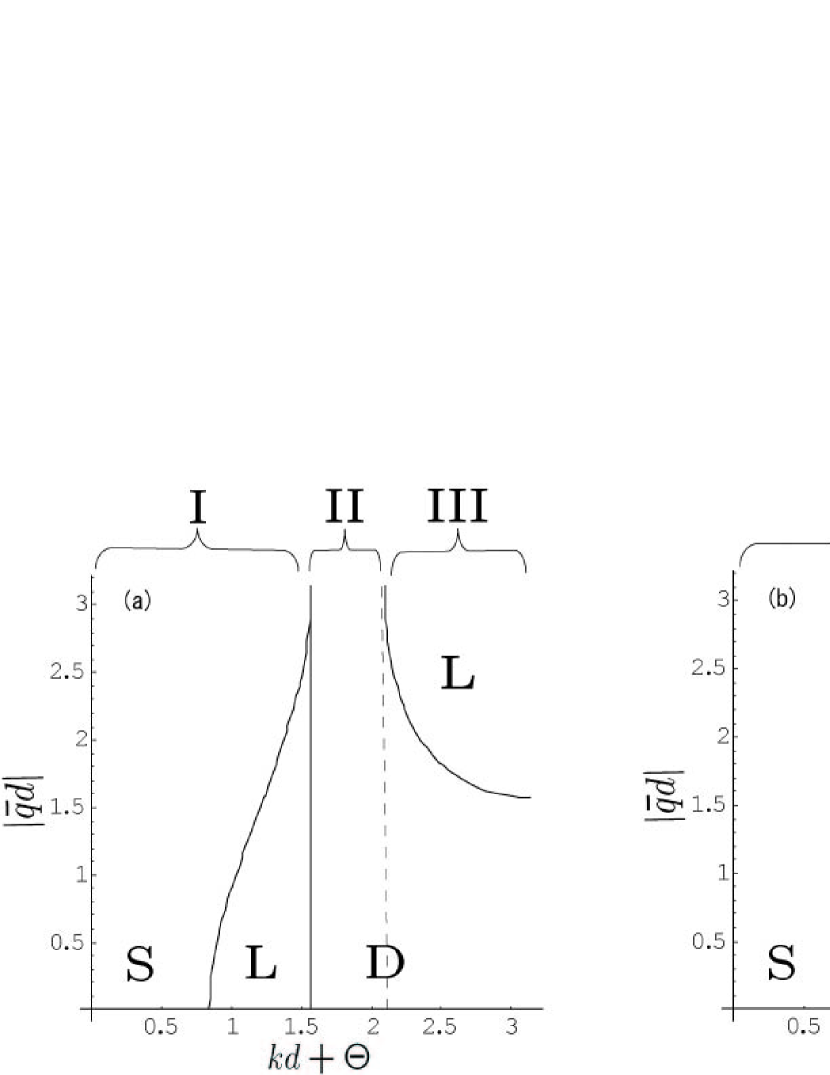
Figure 1: Stability phase diagrams for (a) $n_{\rm c}U/|J|=1$, and (b) $n_{\rm c}U/|J|=2$ in 1D system. The regions S, L and D represent those in which the eigenvalue $\hbar\omega_{\boldsymbol{k\bar{q}}}^{(+)}$ is positive, negative and complex, respectively. We classify the axis of abscissas into three regions, denoted by I, II and III. The eigenvalue is always complex in the region II, while it is always real in the region I. In the region III, it can be real or complex.

IV.1 Some properties of eigenvalues and eigenvectors

We investigate some common properties of the eigenvalues $\hbar\omega_{\boldsymbol{k\bar{q}}}^{(\pm)}$ and eigenvectors $\boldsymbol{x}_{\boldsymbol{k\bar{q}}}^{(\pm)}$.

We find the following two algebraic properties of the non-Hermitian matrix $T_{\boldsymbol{k\bar{q}}}$ which may be expressed as

$$T_{\boldsymbol{k\bar{q}}}=\hbar\omega_{\boldsymbol{k\bar{q}}}^{(1)}\sigma_{0}+(\Lambda_{\boldsymbol{k\bar{q}}}+Un_{\rm c})\sigma_{3}+iUn_{\rm c}\sigma_{2}\,,$$ (62)

where $\sigma_{0}$ is the unit matrix and $\sigma_{i}$ $(i=1,2,3)$ represents $i$-th Pauli matrix.

As the first property, the matrix $T_{\boldsymbol{k\bar{q}}}$ is pseudo-Hermitian:

$$\sigma_{3}T^{\dagger}_{\boldsymbol{k\bar{q}}}\sigma_{3}=T_{\boldsymbol{k\bar{q}}}\,.$$ (63)

Then the inner-product of the doublet eigenvectors is naturally introduced as

$$(\boldsymbol{x},\boldsymbol{x}^{\prime})=\boldsymbol{x}^{\dagger}\sigma_{3}\boldsymbol{x}^{\prime}\,,$$ (64)

since we will later see the orthogonality of eigenvectors with respect to this inner-product, coming from the relation

$$(\boldsymbol{x},T\boldsymbol{x}^{\prime})=(T\boldsymbol{x},\boldsymbol{x}^{\prime})\,,$$ (65)

for any pseudo-Hermitian matrix $T$ in the sense of Eq. (63). Note that the metric with respect to this inner-product is indefinite.

The second property is derived as

$$\sigma_{1}T_{\boldsymbol{k\bar{q}}}\sigma_{1} = \hbar\omega_{\boldsymbol{k\bar{q}}}^{(1)}\sigma_{0}-(\Lambda_{\boldsymbol{k\bar{q}}}+Un_{\rm c})\sigma_{3}-iUn_{\rm c}\sigma_{2}$$ (66)

$$= -\hbar\omega_{\boldsymbol{k}-\boldsymbol{\bar{q}}}^{(1)}\sigma_{0}-(\Lambda_{\boldsymbol{k}-\boldsymbol{\bar{q}}}+Un_{\rm c})\sigma_{3}-iUn_{\rm c}\sigma_{2}$$

$$= -T_{\boldsymbol{k}-\boldsymbol{\bar{q}}}\,.$$

It is also clear from Eqs. (56)–(59) that the eigenvalues $\hbar\omega_{\boldsymbol{k\bar{q}}}^{(\pm)}$ and $\hbar\omega_{\boldsymbol{k}-\boldsymbol{\bar{q}}}^{(\pm)}$ are related to each other,

$$\hbar\omega_{\boldsymbol{k\bar{q}}}^{(\pm)}=-\hbar\omega_{\boldsymbol{k}-\boldsymbol{\bar{q}}}^{(\mp)}\,.$$ (67)

Thus the eigenequations $T_{\boldsymbol{k}-\boldsymbol{\bar{q}}}\boldsymbol{x}_{\boldsymbol{k}-\boldsymbol{\bar{q}}}^{(\pm)}=\hbar\omega_{\boldsymbol{k}-\boldsymbol{\bar{q}}}^{(\pm)}\boldsymbol{x}_{\boldsymbol{k}-\boldsymbol{\bar{q}}}^{(\pm)}$ imply $T_{\boldsymbol{k\bar{q}}}\sigma_{1}\boldsymbol{x}_{\boldsymbol{k}-\boldsymbol{\bar{q}}}^{(\pm)}=\hbar\omega_{\boldsymbol{k\bar{q}}}^{(\mp)}\sigma_{1}\boldsymbol{x}_{\boldsymbol{k}-\boldsymbol{\bar{q}}}^{(\pm)}$, and therefore

$$\boldsymbol{x}_{\boldsymbol{k\bar{q}}}^{(\mp)}=\sigma_{1}\boldsymbol{x}_{\boldsymbol{k}-\boldsymbol{\bar{q}}}^{(\pm)}\,.$$ (68)

We may introduce the traceless part of $T_{\boldsymbol{k\bar{q}}}$ by

$${\tilde{T}}_{\boldsymbol{k\bar{q}}}=(\Lambda_{\boldsymbol{k\bar{q}}}+Un_{\rm c})\sigma_{3}+iUn_{\rm c}\sigma_{2}\,,$$ (69)

for which we have the eigenequations

$${\tilde{T}}_{\boldsymbol{k\bar{q}}}\boldsymbol{x}_{\boldsymbol{k\bar{q}}}^{(\pm)}=\pm\hbar\omega_{\boldsymbol{k\bar{q}}}^{(2)}\boldsymbol{x}_{\boldsymbol{k\bar{q}}}^{(\pm)}\,,$$ (70)

where $\hbar\omega_{\boldsymbol{k\bar{q}}}^{(2)}$ is defined in Eq. (58). Note that $\boldsymbol{x}_{\boldsymbol{k\bar{q}}}^{(\pm)}$ and $\boldsymbol{x}_{\boldsymbol{k-\bar{q}}}^{(\pm)}$ are degenerate states because $\hbar\omega_{\boldsymbol{k\bar{q}}}^{(2)}=\hbar\omega_{\boldsymbol{k-\bar{q}}}^{(2)}$. The matrix ${\tilde{T}}_{\boldsymbol{k\bar{q}}}$ satisfies the algebraic relation,

$$\sigma_{1}{\tilde{T}}_{\boldsymbol{k\bar{q}}}\sigma_{1}=-{\tilde{T}}_{\boldsymbol{k\bar{q}}}\,.$$ (71)

Similarly in the previous paragraph, we easily find that

$${\tilde{T}}_{\boldsymbol{k\bar{q}}}\sigma_{1}\boldsymbol{x}_{\boldsymbol{k\bar{q}}}^{(\pm)}=\mp\hbar\omega_{\boldsymbol{k\bar{q}}}^{(2)}\sigma_{1}\boldsymbol{x}_{\boldsymbol{k\bar{q}}}^{(\pm)}$$ (72)

leading to

$$\boldsymbol{x}_{\boldsymbol{k\bar{q}}}^{(\mp)}=\sigma_{1}\boldsymbol{x}_{\boldsymbol{k\bar{q}}}^{(\pm)}\,.$$ (73)

Thus we can express the four eigenvectors $\boldsymbol{x}_{\boldsymbol{k\bar{q}}}^{(\pm)}$ and $\boldsymbol{x}_{\boldsymbol{k}-\boldsymbol{\bar{q}}}^{(\pm)}$ only by two parameters, say $u_{\boldsymbol{k\bar{q}}}$ and $v_{\boldsymbol{k\bar{q}}}$, except for a trivial phase factor:

$$\boldsymbol{x}_{\boldsymbol{k\bar{q}}}^{(+)}=\boldsymbol{x}_{\boldsymbol{k}-\boldsymbol{\bar{q}}}^{(+)} = \left(\begin{array}[]{c}u_{\boldsymbol{k\bar{q}}}\\ v_{\boldsymbol{k\bar{q}}}\end{array}\right),$$ (76)

$$\boldsymbol{x}_{\boldsymbol{k\bar{q}}}^{(-)}=\boldsymbol{x}_{\boldsymbol{k}-\boldsymbol{\bar{q}}}^{(-)} = \left(\begin{array}[]{c}v_{\boldsymbol{k\bar{q}}}\\ u_{\boldsymbol{k\bar{q}}}\end{array}\right).$$ (79)

IV.2 Real eigenvalues

In this subsection we consider the case where all eigenvalues are real, e.g., the region I in Fig. 1. From Eq. (65), one obtains the following relation

$$(\hbar\omega_{\boldsymbol{k\bar{q}}}^{(s^{\prime})}-\hbar\omega_{\boldsymbol{k\bar{q}}}^{(s)})(\boldsymbol{x}_{\boldsymbol{k\bar{q}}}^{(s)},\boldsymbol{x}_{\boldsymbol{k\bar{q}}}^{(s^{\prime})})=0\,,$$ (80)

where $s$ and $s^{\prime}$ are $+$ or $-$. Therefore we obtain the orthogonality condition

$$(\boldsymbol{x}_{\boldsymbol{k\bar{q}}}^{(-)},\boldsymbol{x}_{\boldsymbol{k\bar{q}}}^{(+)})=(\boldsymbol{x}_{\boldsymbol{k\bar{q}}}^{(+)},\boldsymbol{x}_{\boldsymbol{k\bar{q}}}^{(-)})=0\,.$$ (81)

Noting that $u_{\boldsymbol{k\bar{q}}}$ and $v_{\boldsymbol{k\bar{q}}}$ are real numbers, we may set the normalization condition as

$$u_{\boldsymbol{k\bar{q}}}^{2}-v_{\boldsymbol{k\bar{q}}}^{2} = 1\,.$$ (82)

Then Eqs. (76) and (79) imply that the eigenvectors are normalized with the indefinite metric as

$$(\boldsymbol{x}_{\boldsymbol{k\bar{q}}}^{(+)},\boldsymbol{x}_{\boldsymbol{k\bar{q}}}^{(+)}) = 1\,,$$ (83)

$$(\boldsymbol{x}_{\boldsymbol{k\bar{q}}}^{(-)},\boldsymbol{x}_{\boldsymbol{k\bar{q}}}^{(-)}) = -1\,.$$ (84)

The elements of the eigenvectors are determined explicitly as

$$u_{\boldsymbol{k\bar{q}}} = \sqrt{\frac{1}{2}\left(1+\frac{\Lambda_{\boldsymbol{k\bar{q}}}+Un_{\rm c}}{\hbar\omega_{\boldsymbol{k\bar{q}}}^{(2)}}\right)}\,,$$ (85)

$$v_{\boldsymbol{k\bar{q}}} = -\sqrt{\frac{1}{2}\left(-1+\frac{\Lambda_{\boldsymbol{k\bar{q}}}+Un_{\rm c}}{\hbar\omega_{\boldsymbol{k\bar{q}}}^{(2)}}\right)}\,,$$ (86)

Note that $u_{\boldsymbol{k\bar{0}}}$ and $v_{\boldsymbol{k\bar{0}}}$ are singular in the limit of $\varepsilon\to 0$.

The matrix $T_{\boldsymbol{k\bar{q}}}$ is diagonalized by the matrix $O_{\boldsymbol{k\bar{q}}}$ as

$$O_{\boldsymbol{k\bar{q}}}^{-1}T_{\boldsymbol{k\bar{q}}}O_{\boldsymbol{k\bar{q}}}=\left(\begin{array}[]{cc}\hbar\omega_{\boldsymbol{k\bar{q}}}^{(+)}&0\\ 0&\hbar\omega_{\boldsymbol{k\bar{q}}}^{(-)}\end{array}\right)\,,$$ (89)

where

$$O_{\boldsymbol{k\bar{q}}} = \left(\begin{array}[]{cc}\boldsymbol{x}_{\boldsymbol{k\bar{q}}}^{(+)}&\boldsymbol{x}_{\boldsymbol{k\bar{q}}}^{(-)}\end{array}\right)\,.$$ (91)

The orthonormal conditions (81), (83) and (84) are equivalent to $O_{\boldsymbol{k\bar{q}}}^{\dagger}\sigma_{3}O_{\boldsymbol{k\bar{q}}}=\sigma_{3}$, yielding

$$O_{\boldsymbol{k\bar{q}}}^{-1}=\sigma_{3}O^{\dagger}_{\boldsymbol{k\bar{q}}}\sigma_{3}\,.$$ (92)

The operators, defined by

$$\hat{\boldsymbol{b}}_{\boldsymbol{k\bar{q}}}=\left(\begin{array}[]{c}\hat{b}_{\boldsymbol{k\bar{q}}}\\ \hat{b}_{\boldsymbol{k}-\boldsymbol{\bar{q}}}^{\dagger}\end{array}\right) = O_{\boldsymbol{k\bar{q}}}^{-1}\hat{\boldsymbol{c}}_{\boldsymbol{k\bar{q}}}$$ (95)

$$= \left(\begin{array}[]{cc}u_{\boldsymbol{k\bar{q}}}&-v_{\boldsymbol{k\bar{q}}}\\ -v_{\boldsymbol{k\bar{q}}}&u_{\boldsymbol{k\bar{q}}}\end{array}\right)\left(\begin{array}[]{c}\hat{c}_{\boldsymbol{k\bar{q}}}\\ \hat{c}_{\boldsymbol{k}-\boldsymbol{\bar{q}}}^{\dagger}\end{array}\right)\,,$$ (100)

satisfy the bosonic commutation relations $[\hat{b}_{\boldsymbol{k\bar{q}}},\hat{b}_{\boldsymbol{k\bar{q}^{\prime}}}^{\dagger}]=\delta_{\boldsymbol{\bar{q}\bar{q}^{\prime}}}$ and $[\hat{b}_{\boldsymbol{k\bar{q}}},\hat{b}_{\boldsymbol{k\bar{q}^{\prime}}}]=0$. By using the $\hat{b}$-operators, one obtains the equation of time evolution in a diagonalized form from Eq. (48),

$$i\hbar\frac{d}{dt}\hat{\boldsymbol{b}}_{\boldsymbol{k\bar{q}}}(t)=\left(\begin{array}[]{cc}\hbar\omega_{\boldsymbol{k\bar{q}}}^{(+)}&0\\ 0&-\hbar\omega_{\boldsymbol{k}-\boldsymbol{\bar{q}}}^{(+)}\end{array}\right)\hat{\boldsymbol{b}}_{\boldsymbol{k\bar{q}}}(t)\,,$$ (104)

where Eq. (67) has been made use of. Thus the time evolution of the operator $\hat{b}_{\boldsymbol{k\bar{q}}}$ is simply given as

$$\hat{b}_{\boldsymbol{k\bar{q}}}(t)=\hat{b}_{\boldsymbol{k\bar{q}}}e^{-i\omega_{\boldsymbol{k\bar{q}}}^{(+)}t}\,.$$ (105)

In terms of the ${\hat{b}}$-operators, the unperturbed Hamiltonian (III) is diagonalized as

$$\hat{H}_{0}=\sum_{\boldsymbol{\bar{q}}}\hbar\omega_{\boldsymbol{k\bar{q}}}^{(+)}\hat{b}_{\boldsymbol{k\bar{q}}}^{{\dagger}}\hat{b}_{\boldsymbol{k\bar{q}}}+\rm{const}.$$ (106)

The real eigenvalue $\hbar\omega_{\boldsymbol{k\bar{q}}}^{(+)}$ can be interpreted as an energy of the quasi-particle, and can be negative in our present model. The negative energy causes an energetic instability which is called the Landau instability. For one-dimensional system, the condition of the quasi-particle energy $\hbar\omega_{k\bar{q}}^{(+)}$ being negative is written as

$$\cos^{2}\left(\frac{\bar{q}d}{2}\right)>\cos(kd+\Theta)\left\{\cos(kd+\Theta)+\frac{Un_{\rm c}}{2J}\right\}\,,$$

$$\sin(kd+\Theta)\sin(\bar{q}d)<0$$ (107)

at the limit of $\varepsilon\to 0$.

The operator $\hat{b}_{\boldsymbol{k\bar{0}}}$ represents the zero-mode, as its energy eigenvalue becomes

$$\hbar\omega_{\boldsymbol{k\bar{0}}}=\left(\varepsilon\bar{\epsilon}\right)^{\frac{1}{2}}\left(2Un_{\rm c}+\varepsilon\bar{\epsilon}\right)^{\frac{1}{2}}\rightarrow 0\quad\mbox{as}\quad\varepsilon\rightarrow 0\,,$$ (108)

from Eqs. (LABEL:eq:lambda), (56)–(59). This zero-mode is presumed to be the Nambu-Goldstone (NG) mode appearing in the spontaneous breakdown of global phase symmetry. In order to prove that it is actually the NG mode, one needs to check the Ward-Takahashi relations Enomoto , but this has not been confirmed yet when complex modes appear. The singular elements of $\boldsymbol{x}_{\boldsymbol{k\bar{0}}}^{(\pm)}$ are calculated from Eqs. (85) and (86) as

$$u_{\boldsymbol{k\bar{0}}} = (4\varepsilon\bar{\epsilon})^{-\frac{1}{4}}\left\{\alpha+\frac{(\varepsilon\bar{\epsilon})^{\frac{1}{2}}}{2\alpha}\right\}+O\left(\varepsilon^{\frac{3}{4}}\right)\,,$$ (109)

$$v_{\boldsymbol{k\bar{0}}} = -(4\varepsilon\bar{\epsilon})^{-\frac{1}{4}}\left\{\alpha-\frac{(\varepsilon\bar{\epsilon})^{\frac{1}{2}}}{2\alpha}\right\}+O\left(\varepsilon^{\frac{3}{4}}\right)\,,$$ (110)

where $\alpha=\left(Un_{\rm c}/2\right)^{1/4}$. Regularizing the zero-mode this way, we can include it as a real mode, as was done in our previous works Okumura1 ; MOY .

IV.3 Complex eigenvalues

Next, let us consider the case where all eigenvalues are complex, e.g., the region II in Fig. 1. Then the eigenvalues $\hbar\omega_{\boldsymbol{k\bar{q}}}^{(\pm)}$ are complex conjugate to each other as $\hbar\omega_{\boldsymbol{k\bar{q}}}^{(-)}=\hbar\omega_{\boldsymbol{k\bar{q}}}^{(+)*}$. Now the elements of eigenvector $u_{\boldsymbol{k\bar{q}}}$ and $v_{\boldsymbol{k\bar{q}}}$ become complex numbers. From the relation $(\hbar\omega_{\boldsymbol{k\bar{q}}}^{(s^{\prime})*}-\hbar\omega_{\boldsymbol{k\bar{q}}}^{(s)})(\boldsymbol{x}_{\boldsymbol{k\bar{q}}}^{(s^{\prime})},\boldsymbol{x}_{\boldsymbol{k\bar{q}}}^{(s)})=0$ where the superscript $s$ stands for $\pm$, we obtain

$$(\boldsymbol{x}_{\boldsymbol{k\bar{q}}}^{(+)},\boldsymbol{x}_{\boldsymbol{k\bar{q}}}^{(+)})=(\boldsymbol{x}_{\boldsymbol{k\bar{q}}}^{(-)},\boldsymbol{x}_{\boldsymbol{k\bar{q}}}^{(-)}) = 0\,,$$ (111)

$$(\boldsymbol{x}_{\boldsymbol{k\bar{q}}}^{(-)},\boldsymbol{x}_{\boldsymbol{k\bar{q}}}^{(+)}) = C\,,$$ (112)

where Eqs. (76) and (79) have been used and $C$ turns out to be a pure imaginary constant. In order to fix the constant $C$ in Eq. (112), we take $u_{\boldsymbol{k\bar{q}}}^{2}-v_{\boldsymbol{k\bar{q}}}^{2}=1$ for convenience. Then the expressions for the elements of the eigenvectors in Eqs. (85) and (86) are true for pure imaginary $\hbar\omega_{\boldsymbol{k\bar{q}}}^{(2)}$, and the simple relation,

$$v_{\boldsymbol{k\bar{q}}}^{*}=iu_{\boldsymbol{k\bar{q}}}\,,$$ (113)

is found. This choice corresponds to fixing $C=i$, and the orthonormal conditions (111) and (112) are summarized as

$$O_{\boldsymbol{k\bar{q}}}^{\dagger}\sigma_{3}O_{\boldsymbol{k\bar{q}}}=\sigma_{2}\,,$$ (114)

which derives

$$O_{\boldsymbol{k\bar{q}}}^{-1}=\sigma_{2}O_{\boldsymbol{k\bar{q}}}^{\dagger}\sigma_{3}\,,$$ (115)

Similarly as in Eq (100), we introduce the new operators,

$$\boldsymbol{A}_{\boldsymbol{k\bar{q}}}=\left(\begin{array}[]{c}\hat{A}_{\boldsymbol{k\bar{q}}}\\ \hat{B}_{\boldsymbol{k}-\boldsymbol{\bar{q}}}^{\dagger}\end{array}\right) = O_{\boldsymbol{k\bar{q}}}^{-1}\boldsymbol{c}_{\boldsymbol{k\bar{q}}}$$ (118)

$$= \left(\begin{array}[]{cc}u_{\boldsymbol{k\bar{q}}}&iu_{\boldsymbol{k\bar{q}}}^{*}\\ iu_{\boldsymbol{k\bar{q}}}^{*}&u_{\boldsymbol{k\bar{q}}}\end{array}\right)\left(\begin{array}[]{c}\hat{c}_{\boldsymbol{k\bar{q}}}\\ \hat{c}_{\boldsymbol{k}-\boldsymbol{\bar{q}}}^{\dagger}\end{array}\right).$$ (123)

The operators $\hat{A}_{\boldsymbol{k\bar{q}}}$ and $\hat{B}_{\boldsymbol{k\bar{q}}}$ satisfy the following relations

$$\hat{A}_{\boldsymbol{k\bar{q}}} = i\hat{A}_{\boldsymbol{k}-\boldsymbol{\bar{q}}}^{\dagger}\,,$$ (125)

$$\hat{B}_{\boldsymbol{k\bar{q}}} = -i\hat{B}_{\boldsymbol{k}-\boldsymbol{\bar{q}}}^{\dagger}\,.$$ (126)

The commutation relations among the $\hat{A}_{\boldsymbol{k\bar{q}}}$ and $\hat{B}_{\boldsymbol{k\bar{q}}}$ operators become

$$\big{[}\hat{A}_{\boldsymbol{k\bar{q}}},\hat{B}_{\boldsymbol{k\bar{q}^{\prime}}}^{\dagger}\big{]}=-\big{[}\hat{A}_{\boldsymbol{k\bar{q}}}^{\dagger},\hat{B}_{\boldsymbol{k\bar{q}^{\prime}}}\big{]} = \delta_{\boldsymbol{\bar{q}\bar{q}^{\prime}}}\,,$$ (127)

$$\big{[}\hat{A}_{\boldsymbol{k\bar{q}}},\hat{B}_{\boldsymbol{k\bar{q}^{\prime}}}\big{]}=\big{[}\hat{A}_{\boldsymbol{k\bar{q}}}^{\dagger},\hat{B}_{\boldsymbol{k\bar{q}^{\prime}}}^{\dagger}\big{]} = -i\delta_{\boldsymbol{\bar{q}}-\boldsymbol{\bar{q}^{\prime}}}\,,$$ (128)

$$\big{[}\hat{A}_{\boldsymbol{k\bar{q}}},\hat{A}_{\boldsymbol{k\bar{q}^{\prime}}}^{\dagger}\big{]}=\big{[}\hat{B}_{\boldsymbol{k\bar{q}}},\hat{B}_{\boldsymbol{k\bar{q}^{\prime}}}^{\dagger}\big{]} = 0\,.$$ (129)

The equation of time evolution (48) is reduced to the diagonalized form,

$$i\hbar\frac{d}{dt}\hat{\boldsymbol{A}}_{\boldsymbol{k\bar{q}}}(t)=\left(\begin{array}[]{cc}\hbar\omega_{\boldsymbol{k\bar{q}}}^{(+)}&0\\ 0&\hbar\omega_{\boldsymbol{k\bar{q}}}^{(+)*}\end{array}\right)\hat{\boldsymbol{A}}_{\boldsymbol{k\bar{q}}}(t)\,,$$ (132)

so the operators $\hat{A}_{\boldsymbol{k\bar{q}}}$ and $\hat{B}_{\boldsymbol{k}-\boldsymbol{\bar{q}}}^{\dagger}$ develop in time with the complex frequencies as follows:

$$\hat{A}_{\boldsymbol{k\bar{q}}}(t) = e^{-i\omega_{\boldsymbol{k\bar{q}}}^{(+)}t}\hat{A}_{\boldsymbol{k\bar{q}}}\,,$$ (133)

$$\hat{B}_{\boldsymbol{k}-\boldsymbol{\bar{q}}}^{{\dagger}}(t) = e^{-i\omega_{\boldsymbol{k\bar{q}}}^{(+)*}t}\hat{B}_{\boldsymbol{k}-\boldsymbol{\bar{q}}}^{{\dagger}}\,.$$ (134)

The unperturbed Hamiltonian (III) is reduced to

$$\hat{H}_{0}=\sum_{\boldsymbol{\bar{q}}}\left(\frac{\hbar\omega_{\boldsymbol{k\bar{q}}}^{(+)}}{2}\hat{B}_{\boldsymbol{k\bar{q}}}^{{\dagger}}\hat{A}_{\boldsymbol{k\bar{q}}}+\frac{\hbar\omega_{\boldsymbol{k\bar{q}}}^{(+)*}}{2}\hat{A}_{\boldsymbol{k\bar{q}}}^{{\dagger}}\hat{B}_{\boldsymbol{k\bar{q}}}\right)\,.$$ (135)

This way the Hamiltonian for complex modes is put into a diagonal form, but does not have a representation in a Fock space, and the complex eigenvalue can not be interpreted as a quasi-particle energy.

IV.4 Hamiltonian and canonical commutation relations

Generally both real and complex eigenvalues can coexist, e.g., the region III in Fig. 1. In such a case, the arguments in the preceding two subsections give the following Hamiltonian in a diagonal form,

$$\hat{H}_{0} = \sum_{\boldsymbol{\bar{q}_{\rm c}}}\left(\frac{\hbar\omega_{\boldsymbol{k\bar{q}_{\rm c}}}^{(+)}}{2}\hat{B}_{\boldsymbol{k\bar{q}_{\rm c}}}^{{\dagger}}\hat{A}_{\boldsymbol{k\bar{q}_{\rm c}}}+\frac{\hbar\omega_{\boldsymbol{k\bar{q}_{\rm c}}}^{(+)*}}{2}\hat{A}_{\boldsymbol{k\bar{q}_{\rm c}}}^{{\dagger}}\hat{B}_{\boldsymbol{k\bar{q}_{\rm c}}}\right)$$ (136)

$$\hskip 28.45274pt{}+\sum_{\boldsymbol{\bar{q}_{\rm r}}}\hbar\omega_{\boldsymbol{k\bar{q}_{\rm r}}}^{(+)}\hat{b}_{\boldsymbol{k\bar{q}_{\rm r}}}^{{\dagger}}\hat{b}_{\boldsymbol{k\bar{q}_{\rm r}}}+\rm{const}.,$$

where the Bloch wave number $\boldsymbol{\bar{q}}$ is distinguished by its subscript depending on the property of the eigenvalue, i.e., $\boldsymbol{\bar{q}_{\rm r}}$ for real eigenvalue and $\boldsymbol{\bar{q}_{\rm c}}$ for complex one.

The operator $\hat{c}_{\boldsymbol{k\bar{q}}}$ is now written in terms of $\hat{b}_{\boldsymbol{k\bar{q}}}$, $\hat{A}_{\boldsymbol{k\bar{q}}}$ and $\hat{B}_{\boldsymbol{k}-\boldsymbol{\bar{q}}}^{\dagger}$ as

$$\hat{c}_{\boldsymbol{k\bar{q}_{\rm r}}}(t) = u_{\boldsymbol{k\bar{q}_{\rm r}}}\hat{b}_{\boldsymbol{k\bar{q}_{\rm r}}}e^{-i\omega_{\boldsymbol{k\bar{q}_{\rm r}}}^{(+)}t}+v_{\boldsymbol{k\bar{q}_{\rm r}}}\hat{b}_{\boldsymbol{k}-\boldsymbol{\bar{q}_{\rm r}}}^{{\dagger}}e^{i\omega_{\boldsymbol{k}-\boldsymbol{\bar{q}_{\rm r}}}^{(+)}t}\,,$$

$$\hat{c}_{\boldsymbol{k\bar{q}_{\rm c}}}(t) = u_{\boldsymbol{k\bar{q}_{\rm c}}}\hat{A}_{\boldsymbol{k\bar{q}_{\rm c}}}e^{-i\omega_{\boldsymbol{k\bar{q}_{\rm c}}}^{(+)}t}-iu^{*}_{\boldsymbol{k\bar{q}_{\rm c}}}\hat{B}_{\boldsymbol{k}-\boldsymbol{\bar{q}_{\rm c}}}^{{\dagger}}e^{-i\omega_{\boldsymbol{k\bar{q}_{\rm c}}}^{(+)*}t}\,.$$

The expansion of the field operator Eq. (47) becomes

$$\hat{\phi}(x) = \sum_{\boldsymbol{\bar{q}_{\rm r}}}\left(u_{\boldsymbol{k\bar{q}_{\rm r}}}f_{\boldsymbol{k\bar{q}_{\rm r}}}(\boldsymbol{x})\hat{b}_{\boldsymbol{k\bar{q}_{\rm r}}}e^{-i\omega_{\boldsymbol{k\bar{q}_{\rm r}}}^{(+)}t}+v_{\boldsymbol{k\bar{q}_{\rm r}}}f_{\boldsymbol{k\bar{q}_{\rm r}}}(\boldsymbol{x})\hat{b}_{\boldsymbol{k}-\boldsymbol{\bar{q}_{\rm r}}}^{{\dagger}}e^{i\omega_{\boldsymbol{k}-\boldsymbol{\bar{q}_{\rm r}}}^{(+)}t}\right)$$ (137)

$${}+\sum_{\boldsymbol{\bar{q}_{\rm c}}}\left(u_{\boldsymbol{k\bar{q}_{\rm c}}}f_{\boldsymbol{k\bar{q}_{\rm c}}}(\boldsymbol{x})\hat{A}_{\boldsymbol{k\bar{q}_{\rm c}}}e^{-i\omega_{\boldsymbol{k\bar{q}_{\rm c}}}^{(+)}t}-iu^{*}_{\boldsymbol{k\bar{q}_{\rm c}}}f_{\boldsymbol{k\bar{q}_{\rm c}}}(\boldsymbol{x})\hat{B}_{\boldsymbol{k}-\boldsymbol{\bar{q}_{\rm c}}}^{{\dagger}}e^{-i\omega_{\boldsymbol{k\bar{q}_{\rm c}}}^{(+)*}t}\right)\,.$$

One can easily check that the field operators satisfy the CCRs in the first band,

$$\big{[}\hat{\phi}(\boldsymbol{x},t),\hat{\phi}^{{\dagger}}(\boldsymbol{x}^{\prime},t)\big{]} = \delta(\boldsymbol{x}-\boldsymbol{x}^{\prime})\,,$$

$$\big{[}\hat{\phi}(\boldsymbol{x},t),\hat{\phi}(\boldsymbol{x}^{\prime},t)\big{]} = \big{[}\hat{\phi}^{{\dagger}}(\boldsymbol{x},t),\hat{\phi}^{{\dagger}}(\boldsymbol{x}^{\prime},t)\big{]}=0\,.$$ (138)

IV.5 Eigenstate of complex mode

In order to find eigenstates of the Hamiltonian (136) we introduce the operator that transforms $\hat{c}_{\boldsymbol{k\bar{q}}}$ to $\hat{b}_{\boldsymbol{k\bar{q}}}$ or $\hat{A}_{\boldsymbol{k\bar{q}}}$ and $\hat{B}_{\boldsymbol{k\bar{q}}}$, defined by

$$\hat{V}=\exp\Big{[}\sum_{\boldsymbol{\bar{q}}}i\theta_{\boldsymbol{k\bar{q}}}\hat{G}_{\boldsymbol{k\bar{q}}}\Big{]}\,,$$ (139)

where $\hat{G}_{\boldsymbol{k\bar{q}}}$ is

$$\hat{G}_{\boldsymbol{k\bar{q}}}=i\left(\hat{c}_{\boldsymbol{k\bar{q}}}\hat{c}_{\boldsymbol{k}-\boldsymbol{\bar{q}}}-\hat{c}_{\boldsymbol{k\bar{q}}}^{{\dagger}}\hat{c}_{\boldsymbol{k}-\boldsymbol{\bar{q}}}^{{\dagger}}\right)\,.$$ (140)

Note that $\theta_{\boldsymbol{k\bar{q}}}$ is in general a complex number, and it is written by a pair of real numbers, $\theta^{\rm R}_{\boldsymbol{k\bar{q}}}$ and $\theta^{\rm I}_{\boldsymbol{k\bar{q}}}$, as

$$\theta_{\boldsymbol{k\bar{q}}}=\theta_{\boldsymbol{k\bar{q}}}^{\rm R}+i\theta_{\boldsymbol{k\bar{q}}}^{\rm I}\,,$$ (141)

so the operator $\hat{V}$ is not unitary unless the parameter $\theta_{\boldsymbol{k\bar{q}}}^{\rm I}$ vanishes identically. As is well known, the operator $\hat{V}$ gives rise to the Bogoliubov transformation when all the parameters $\theta_{\boldsymbol{k\bar{q}}}$ are real Umezawa . Even for complex $\theta_{\boldsymbol{k\bar{q}}}$, the transformation generated by the operator $\hat{V}$ may be written down as

$$\hat{V}\left(\begin{array}[]{c}\hat{c}_{\boldsymbol{k\bar{q}}}\\ \hat{c}_{\boldsymbol{k}-\boldsymbol{\bar{q}}}^{\dagger}\end{array}\right)\hat{V}^{-1}=O^{-1}(\theta_{\boldsymbol{k\bar{q}}})\left(\begin{array}[]{c}\hat{c}_{\boldsymbol{k\bar{q}}}\\ \hat{c}_{\boldsymbol{k}-\boldsymbol{\bar{q}}}^{\dagger}\end{array}\right),$$ (146)

where

$$O^{-1}(\theta_{\boldsymbol{k\bar{q}}})=\left(\begin{array}[]{cc}\cosh(\theta_{\boldsymbol{k\bar{q}}})&-\sinh(\theta_{\boldsymbol{k\bar{q}}})\\ -\sinh(\theta_{\boldsymbol{k\bar{q}}})&\cosh(\theta_{\boldsymbol{k\bar{q}}})\end{array}\right).$$ (149)

Now, we look for the parameter values of $\theta_{\boldsymbol{k\bar{q}}}$ for which the above $O^{-1}(\theta_{\boldsymbol{k\bar{q}}})$ reproduces the matrix $O_{\boldsymbol{k\bar{q}}}^{-1}\hat{\boldsymbol{c}}_{\boldsymbol{k\bar{q}}}$ in Eq. (100) for real eigenvalues or in Eq. (123) for complex ones. Simple calculations show

$$\theta_{\boldsymbol{k\bar{q}}}^{\rm I} = 0\,,$$ (150)

$$\cosh\theta_{\boldsymbol{k\bar{q}}}^{\rm R} = u_{\boldsymbol{k\bar{q}}}\,,$$ (151)

$$\sinh\theta_{\boldsymbol{k\bar{q}}}^{\rm R} = v_{\boldsymbol{k\bar{q}}}$$ (152)

for real eigenvalues, and

$$\theta_{\boldsymbol{k\bar{q}}}^{\rm I}=-\frac{\pi}{4}\,,$$ (153)

$$\frac{1}{\sqrt{2}}\left(\cosh\theta_{\boldsymbol{k\bar{q}}}^{\rm R}-i\sinh\theta_{\boldsymbol{k\bar{q}}}^{\rm R}\right)=u_{\boldsymbol{k\bar{q}}}$$ (154)

for complex ones.

Let us focus on the complex eigenvalue sector in which we have explicitly

$$\hat{A}_{\boldsymbol{k\bar{q}_{\rm c}}} = \hat{V}\hat{c}_{\boldsymbol{k\bar{q}_{\rm c}}}\hat{V}^{-1}\,,$$ (155)

$$\hat{B}_{\boldsymbol{k}-\boldsymbol{\bar{q}_{\rm c}}}^{{\dagger}} = \hat{V}\hat{c}_{\boldsymbol{k}-\boldsymbol{\bar{q}_{\rm c}}}^{{\dagger}}\hat{V}^{-1}\,,$$ (156)

and

$$\hat{A}_{\boldsymbol{k\bar{q}_{\rm c}}}^{{\dagger}} = V^{-1{\dagger}}\hat{c}_{\boldsymbol{k\bar{q}_{\rm c}}}^{{\dagger}}V^{{\dagger}}$$ (157)

$$= -i\hat{A}_{\boldsymbol{k}-\boldsymbol{\bar{q}_{\rm c}}}\,,$$

$$\hat{B}_{\boldsymbol{k}-\boldsymbol{\bar{q}_{\rm c}}} = V^{-1{\dagger}}\hat{c}_{\boldsymbol{k}-\boldsymbol{\bar{q}_{\rm c}}}V^{{\dagger}}$$ (158)

$$= -i\hat{B}_{\boldsymbol{k\bar{q}_{\rm c}}}^{{\dagger}}\,.$$

We first define new vacuum states by

$$|0\rangle_{A} = \hat{V}|0\rangle_{c}\,,$$ (159)

$$|0\rangle_{B} = \hat{V}^{-1{\dagger}}|0\rangle_{c}\,,$$ (160)

and

$${}_{A}\langle 0| = {}_{c}\langle 0|\hat{V}^{{\dagger}}\,,$$ (161)

$${}_{B}\langle 0| = {}_{c}\langle 0|\hat{V}^{-1}\,,$$ (162)

where $|0\rangle_{c}$ is the vacuum of $\hat{c}_{\boldsymbol{k\bar{q}}}$. They are annihilated by $\hat{A}_{\boldsymbol{k\bar{q}_{\rm c}}}$, $\hat{A}_{\boldsymbol{k\bar{q}_{\rm c}}}^{{\dagger}}$, $\hat{B}_{\boldsymbol{k\bar{q}_{\rm c}}}$ and $\hat{B}_{\boldsymbol{k\bar{q}_{\rm c}}}^{{\dagger}}$ as follows:

$$\hat{A}_{\boldsymbol{k\bar{q}_{\rm c}}}|0\rangle_{A}=\hat{A}_{\boldsymbol{k\bar{q}_{\rm c}}}^{{\dagger}}|0\rangle_{A}=0\,,$$ (163)

$$\hat{B}_{\boldsymbol{k\bar{q}_{\rm c}}}|0\rangle_{B}=\hat{B}_{\boldsymbol{k\bar{q}_{\rm c}}}^{\dagger}|0\rangle_{B}=0\,,$$ (164)

and

$${}_{A}\langle 0|\hat{A}_{\boldsymbol{k\bar{q}_{\rm c}}}={}_{A}\langle 0|\hat{A}_{\boldsymbol{k\bar{q}_{\rm c}}}^{{\dagger}}=0\,,$$ (165)

$${}_{B}\langle 0|\hat{B}_{\boldsymbol{k\bar{q}_{\rm c}}}={}_{B}\langle 0|\hat{B}_{\boldsymbol{k\bar{q}_{\rm c}}}^{{\dagger}}=0\,.$$ (166)

From the commutation relations (127)–(129), it turns out that these states are eigenstates of the Hamiltonian $\hat{H}_{0}$,

$$\hat{H}_{0}|0\rangle_{A} = -\left(\sum_{\boldsymbol{\bar{q}_{\rm c}}}\frac{\hbar\omega_{\boldsymbol{k\bar{q}_{\rm c}}}^{(+)*}}{2}\right)|0\rangle_{A}\,,$$ (167)

$$\hat{H}_{0}|0\rangle_{B} = -\left(\sum_{\boldsymbol{\bar{q}_{\rm c}}}\frac{\hbar\omega_{\boldsymbol{k\bar{q}_{\rm c}}}^{(+)}}{2}\right)|0\rangle_{B}\,.$$ (168)

Note the relations for ${}_{A}\langle 0|$ and ${}_{B}\langle 0|$ ,

$${}_{A}\langle 0|\hat{H}_{0} = -\left(\sum_{\boldsymbol{\bar{q}_{\rm c}}}\frac{\hbar\omega_{\boldsymbol{k\bar{q}_{\rm c}}}^{(+)}}{2}\right){}_{A}\langle 0|\,,$$ (169)

$${}_{B}\langle 0|\hat{H}_{0} = -\left(\sum_{\boldsymbol{\bar{q}_{\rm c}}}\frac{\hbar\omega_{\boldsymbol{k\bar{q}_{\rm c}}}^{(+)*}}{2}\right){}_{B}\langle 0|\,.$$ (170)

The commutation relations (127) suggest us to introduce the following excited states through cyclic operations of ${\hat{B}}^{\dagger}$ on $|0\rangle_{A}$ and of ${\hat{A}}^{\dagger}$ on $|0\rangle_{B}$:

$$|N_{\rm C}\rangle_{A} \equiv |n_{\boldsymbol{\bar{q}_{{\rm c}\boldsymbol{1}}}}\cdots n_{\boldsymbol{\bar{q}_{\rm{c}\boldsymbol{i}}}}\rangle_{A}$$ (171)

$$= \prod_{\boldsymbol{\bar{q}_{{\rm c}{\boldsymbol{j}}}}}\sqrt{\frac{1}{n_{\boldsymbol{\bar{q}_{{\rm c}{\boldsymbol{j}}}}}!}}(\hat{B}_{\boldsymbol{k\bar{q}_{{\rm c}{\boldsymbol{j}}}}}^{{\dagger}})^{n_{\boldsymbol{\bar{q}_{{\rm c}{\boldsymbol{j}}}}}}|0\rangle_{A}\,,$$

$$|N_{\rm C}\rangle_{B} \equiv |n_{\boldsymbol{\bar{q}_{\rm c1}}}\cdots n_{\boldsymbol{\bar{q}_{{\rm c}{\boldsymbol{i}}}}}\rangle_{B}$$ (172)

$$= \prod_{\boldsymbol{\bar{q}_{{\rm c}{\boldsymbol{j}}}}}\sqrt{\frac{1}{n_{\boldsymbol{\bar{q}_{{\rm c}{\boldsymbol{j}}}}}!}}(\hat{A}_{\boldsymbol{k\bar{q}_{{\rm c}{\boldsymbol{j}}}}}^{{\dagger}})^{n_{\boldsymbol{\bar{q}_{{\rm c}{\boldsymbol{j}}}}}}|0\rangle_{B}\,.$$

These excited states are also eigenstates of $\hat{H}_{0}$ as

$$\hat{H}_{0}|N_{\rm C}\rangle_{A} = \sum_{\boldsymbol{\bar{q}_{\rm c}}}\left(n_{\boldsymbol{\bar{q}_{\rm c}}}\hbar\omega_{\boldsymbol{k\bar{q}_{\rm c}}}^{(+)}-\frac{\hbar\omega_{\boldsymbol{k\bar{q}_{\rm c}}}^{(+)*}}{2}\right)|N_{\rm C}\rangle_{A}\,,$$

$$\hat{H}_{0}|N_{\rm C}\rangle_{B} = \sum_{\boldsymbol{\bar{q}_{\rm c}}}\left(n_{\boldsymbol{\bar{q}_{\rm c}}}\hbar\omega_{\boldsymbol{k\bar{q}_{\rm c}}}^{(+)*}-\frac{\hbar\omega_{\boldsymbol{k\bar{q}_{\rm c}}}^{(+)}}{2}\right)|N_{\rm C}\rangle_{B}\,.$$

Let us evaluate ${}_{A}\langle 0|0\rangle_{A}$, which is rewritten as

$${}_{A}\langle 0|0\rangle_{A} = {}_{c}\langle 0|\hat{W}|0\rangle_{c}$$

$$\hat{W} = \exp\Big{[}i\frac{\pi}{2}\sum_{\boldsymbol{\bar{q}_{\rm c}}}\left(\hat{c}_{\boldsymbol{k\bar{q}_{\rm c}}}\hat{c}_{\boldsymbol{k}-\boldsymbol{\bar{q}_{\rm c}}}-\hat{c}_{\boldsymbol{k\bar{q}_{\rm c}}}^{{\dagger}}\hat{c}_{\boldsymbol{k}-\boldsymbol{\bar{q}_{\rm c}}}^{{\dagger}}\right)\Big{]}\,.$$

Consider a state $|\xi\rangle$,

$$|\xi\rangle \equiv \exp\Big{[}\sum_{\boldsymbol{\bar{q}_{\rm c}}}-\xi\left(\hat{c}_{\boldsymbol{k\bar{q}_{\rm c}}}\hat{c}_{\boldsymbol{k}-\boldsymbol{\bar{q}_{\rm c}}}-\hat{c}_{\boldsymbol{k\bar{q}_{\rm c}}}^{{\dagger}}\hat{c}_{\boldsymbol{k}-\boldsymbol{\bar{q}_{\rm c}}}^{{\dagger}}\right)\Big{]}|0\rangle_{c}$$

$$= \exp\Big{[}-\ln\cosh\xi+\sum_{\boldsymbol{\bar{q}_{\rm c}}}\hat{c}_{\boldsymbol{k\bar{q}_{\rm c}}}^{{\dagger}}\hat{c}_{\boldsymbol{k}-\boldsymbol{\bar{q}_{\rm c}}}^{{\dagger}}\tanh\xi\Big{]}|0\rangle_{c}\,,$$

then we have the relation ${}_{A}\langle 0|0\rangle_{A}={}_{c}\langle 0|\xi=-i\pi/2\rangle$. Obviously ${}_{c}\langle 0|\xi\rangle$ diverges at the limit $\xi\to-i\pi/2$, so does ${}_{A}\langle 0|0\rangle_{A}$. Similarly ${}_{B}\langle 0|0\rangle_{B}$ is also divergent.

Using Eqs. (159)–(162), one easily derives

$${}_{A}\langle 0|0\rangle_{B} = 1\,,$$ (177)

$${}_{B}\langle 0|0\rangle_{A} = 1\,.$$ (178)

The commutation relations in Eqs. (127)–(129) lead to

$${}_{A}\langle N_{\rm C}^{{}^{\prime}}|N_{\rm C}\rangle_{B}=\prod_{\boldsymbol{\bar{q}_{{\rm c}{\boldsymbol{j}}}}}\delta_{n^{\prime}_{\boldsymbol{\bar{q}_{{\rm c}{\boldsymbol{j}}}}}n_{\boldsymbol{\bar{q}_{{\rm c}{\boldsymbol{j}}}}}}\,,$$ (179)

$${}_{B}\langle N_{\rm C}^{{}^{\prime}}|N_{\rm C}\rangle_{A}=\prod_{\boldsymbol{\bar{q}_{{\rm c}{\boldsymbol{j}}}}}\delta_{n^{\prime}_{\boldsymbol{\bar{q}_{{\rm c}{\boldsymbol{j}}}}}n_{\boldsymbol{\bar{q}_{{\rm c}{\boldsymbol{j}}}}}}\,.$$ (180)

Let us rewrite the completeness relation in the complex mode sector, using the complete set of $|N_{\rm C}\rangle_{c}$,

$${\bf 1}_{\rm C}=\sum_{N_{\rm C}}|N_{\rm C}\rangle_{c}\,\,{}_{c}\langle N_{\rm C}|\,,$$ (181)

where ${\bf 1}_{\rm C}$ is the identity operator in the complex sector and

$$|N_{\rm C}\rangle_{c}\equiv\prod_{\boldsymbol{\bar{q}_{{\rm c}{\boldsymbol{j}}}}}\sqrt{\frac{1}{n_{\boldsymbol{\bar{q}_{{\rm c}{\boldsymbol{j}}}}}!}}(\hat{c}_{\boldsymbol{k\bar{q}_{{\rm c}{\boldsymbol{j}}}}}^{{\dagger}})^{n_{\boldsymbol{\bar{q}_{{\rm c}{\boldsymbol{j}}}}}}|0\rangle_{c}\,.$$ (182)

Having $\hat{V}$ and $\hat{V}^{-1}$ operate on Eq. (181) from the left and right, respectively, we obtain the completeness relation using the states $|n_{\boldsymbol{\bar{q}_{{\rm c}{\boldsymbol{1}}}}},\cdots,n_{\boldsymbol{\bar{q}_{{\rm c}{\boldsymbol{i}}}}}\rangle_{A}$ and ${}_{B}\langle n_{\boldsymbol{\bar{q}_{{\rm c}{\boldsymbol{1}}}}},\cdots,n_{\boldsymbol{\bar{q}_{{\rm c}{\boldsymbol{i}}}}}|$ as

$${\bf 1}_{\rm C} = \sum_{N_{\rm C}}\hat{V}|N_{\rm C}\rangle_{c}\,\,{}_{c}\langle N_{\rm C}|\hat{V}^{-1}$$ (183)

$$= \sum_{N_{\rm C}}|N_{\rm C}\rangle_{A}\,\,{}_{B}\langle N_{\rm C}|\,.$$

Similarly another relation using the states $|N_{\rm C}\rangle_{B}$ and ${}_{A}\langle N_{\rm C}|$ follows:

$${\bf 1}_{\rm C}=\sum_{N_{\rm C}}|N_{\rm C}\rangle_{B}\,\,{}_{A}\langle N_{\rm C}|.$$ (184)

One may say that a natural conjugate of $|N_{\rm C}\rangle_{A}$ is ${}_{B}\langle N_{\rm C}|$ and vice versa MOSY .

V Physical States

In the previous section, we have “diagonalized” the unperturbed Hamiltonian including complex eigenvalues and have found its eigenstates. The state space is not a simple Fock one. We need to impose appropriate conditions to construct a restricted physical state space. In QFT, unstable behaviors of system are described in a stable picture such as the Beliaev process. We should now establish a stable particle picture specified by the unperturbed Hamiltonian, and the decay processes are described as the higher order of perturbation. We presume that unstable behaviors of the BECs in optical lattices occur due to external perturbation.

As in Ref.  MOSY , we require the following physical state conditions (PSCs).

$${\rm i}) \langle\overline{\Omega}|\hat{\Psi}(x)|\Omega\rangle=v(\boldsymbol{x})\,,$$

$${\rm ii}) \langle\overline{\Omega}|\hat{\Psi}^{\dagger}(x)\hat{\Psi}(x)|\Omega\rangle\text{ is time-independent}\,,$$

$${\rm iii}) \langle\overline{\Omega}|\hat{G}|\Omega\rangle \hat{G}$$ is real, when is any Hermitian operator ,

$${\rm iv}) \langle\overline{\Omega}|\Omega\rangle=1\,,$$

where $\langle\overline{\Omega}|$ is the natural conjugate of $|\Omega\rangle$. If $\langle\overline{\Omega}|$ and $|\Omega\rangle$ satisfy the above four conditions, we call them physical states. The conditions i) and ii) mean that the order parameter and density distribution are stationary without perturbation. The condition iii) guarantees that the expectation value of any Hermitian operator can interpreted as physical quantity. The condition iv) is necessary for the probability interpretation. The vacuum states which satisfy the PSCs are obtained as direct sum of $|0\rangle_{A}$ and $|0\rangle_{B}$ ,

$$|0\rangle_{\oplus} \equiv \frac{1}{\sqrt{2}}\left(|0\rangle_{A}\oplus|0\rangle_{B}\right)\,,$$ (185)

$${}_{\oplus}\langle 0| \equiv \frac{1}{\sqrt{2}}\left({}_{B}\langle 0|\oplus{}_{A}\langle 0|\right).$$ (186)

The proof that these direct sum states satisfy PSCs is given in Ref. MOSY . Here we add that the direct sum of the excited states $|N_{\rm C}\rangle_{A}$ and $|N_{\rm C}\rangle_{B}$ are also physical states,

$$|N_{\rm C}\rangle_{\oplus} \equiv \frac{1}{\sqrt{2}}\left(|N_{\rm C}\rangle_{A}\oplus|N_{\rm C}\rangle_{B}\right)\,,$$ (187)

$${}_{\oplus}\langle N_{\rm C}| \equiv \frac{1}{\sqrt{2}}\left({}_{B}\langle N_{\rm C}|\oplus{}_{A}\langle N_{\rm C}|\right)\,.$$ (188)

VI Linear Response

So far, we have developed the description of QFT with complex eigenvalues. But complex eigenvalues are not directly connected with the instability of a condensate. In this section, we discuss the dynamics of the system with complex eigenvalues, studying the response of a condensate against external perturbation. To derive theoretical expressions is straightforward in the linear response theory (LRT) Kubo with our formulation of QFT. We also show numerical results of LRT and compare them with those from the TDGP equation, concretely those from the discrete nonlinear Schrödinger equation (DNSE) which is obtained by applying the tight-binding approximation to the TDGP equation DNLS ; DNLS2 .

VI.1 Formula

The field operator $\hat{\Psi}$ is expanded in terms of the Wannier functions as $\hat{\Psi}=v_{\boldsymbol{k}}+\sum_{\boldsymbol{i}}\hat{a}_{\boldsymbol{ki}}w_{\boldsymbol{ki}}$. The particle number operator $\hat{N}=\int\!d^{3}x\,\hat{\Psi}^{{\dagger}}\hat{\Psi}$ is written as

$$\hat{N} = \sum_{\boldsymbol{i}}\rho_{\boldsymbol{i}}(t)\,,$$ (189)

$$\hat{\rho}_{\boldsymbol{i}}(t) = \hat{\rho}_{\boldsymbol{i}}^{(0)}(t)+\hat{\rho}_{\boldsymbol{i}}^{(\mathrm{ex})}(t)\,,$$ (190)

$$\hat{\rho}_{\boldsymbol{i}}^{(0)}(t) = n_{\rm c}+n_{\rm c}^{\frac{1}{2}}e^{-i\boldsymbol{k\cdot x_{\boldsymbol{i}}}}\hat{a}_{\boldsymbol{ki}}(t)+n_{\rm c}^{\frac{1}{2}}e^{i\boldsymbol{k\cdot x_{\boldsymbol{i}}}}\hat{a}_{\boldsymbol{ki}}^{{\dagger}}(t)\,,$$

$$\hat{\rho}_{\boldsymbol{i}}^{(\mathrm{ex})}(t) = \hat{a}_{\boldsymbol{ki}}^{{\dagger}}(t)\hat{a}_{\boldsymbol{ki}}(t)\,,$$ (192)

where $\rho_{\boldsymbol{i}}(t)$ is the particle density operator at the ${\boldsymbol{i}}$-th site, and $\hat{a}_{\boldsymbol{ki}}(t)$ is

$$\hat{a}_{\boldsymbol{ki}}(t) = \sum_{\boldsymbol{\bar{q}_{\rm r}}}\frac{e^{i(\boldsymbol{k}+\boldsymbol{\bar{q}_{\rm r}})\cdot\boldsymbol{x}_{\boldsymbol{i}}}}{I_{\rm s}^{\frac{1}{2}}}\hat{c}_{\boldsymbol{k\bar{q}_{\rm r}}}(t)+\sum_{\boldsymbol{\bar{q}_{\rm c}}}\frac{e^{i(\boldsymbol{k}+\boldsymbol{\bar{q}_{\rm c}})\cdot\boldsymbol{x}_{\boldsymbol{i}}}}{I_{\rm s}^{\frac{1}{2}}}\hat{c}_{\boldsymbol{k\bar{q}_{\rm c}}}(t)\,,$$

where

$$\hat{c}_{\boldsymbol{k\bar{q}}_{\rm r}}(t) = u_{\boldsymbol{k\bar{q}_{\rm r}}}\hat{b}_{\boldsymbol{k\bar{q}_{\rm r}}}e^{-i\omega_{\boldsymbol{k\bar{q}_{\rm r}}}^{(+)}t}+v_{\boldsymbol{k\bar{q}_{\rm r}}}\hat{b}_{\boldsymbol{k}-\boldsymbol{\bar{q}_{\rm r}}}^{{\dagger}}e^{i\omega_{\boldsymbol{k}-\boldsymbol{\bar{q}_{\rm r}}}^{(+)}t}\,,$$

$$\hat{c}_{\boldsymbol{k\bar{q}}_{\rm c}}(t) = u_{\boldsymbol{k\bar{q}_{\rm c}}}\hat{A}_{\boldsymbol{k\bar{q}_{\rm c}}}e^{-i\omega_{\boldsymbol{k\bar{q}_{\rm c}}}^{(+)}t}-iu_{\boldsymbol{k\bar{q}_{\rm c}}}^{*}\hat{B}_{\boldsymbol{k}-\boldsymbol{\bar{q}_{\rm c}}}^{{\dagger}}e^{-i\omega_{\boldsymbol{k\bar{q}_{\rm c}}}^{(+)*}t}\,.$$

We consider the external perturbation as

$$\hat{H}_{\mathrm{per}}(t) = \int\!d^{3}x\,\hat{\Psi}^{{\dagger}}V_{\mathrm{per}}(\boldsymbol{x},t)\hat{\Psi}$$ (196)

$$= \sum_{\boldsymbol{i,j}}\delta V_{\boldsymbol{ij}}(t)\left(n_{\rm c}+n_{\rm c}^{\frac{1}{2}}e^{-i\boldsymbol{k\cdot x_{\boldsymbol{i}}}}\hat{a}_{\boldsymbol{kj}}\right.$$

$$\left.\hskip 22.76228pt{}+n_{\rm c}^{\frac{1}{2}}e^{i\boldsymbol{k\cdot x}_{\boldsymbol{j}}}\hat{a}_{\boldsymbol{ki}}^{{\dagger}}+\hat{a}_{\boldsymbol{ki}}^{{\dagger}}\hat{a}_{\boldsymbol{kj}}\right)\,,$$

where

$$\delta V_{\boldsymbol{ij}}(t) = \int\!d^{3}x\,w_{\boldsymbol{ki}}^{*}\delta V_{\mathrm{per}}w_{\boldsymbol{kj}}\,.$$ (197)

The function $\delta V_{\mathrm{per}}(\boldsymbol{x},t)$ represents the time-dependent modification of trap. We use the on-site approximation for $\delta V_{\boldsymbol{ij}}(t)$. The external perturbative Hamiltonian (196) becomes

$$\hat{H}_{\mathrm{per}}(t)=\sum_{\boldsymbol{i}}\delta V_{\boldsymbol{i}}(t)\hat{\rho}_{\boldsymbol{i}}(t)\,,$$ (198)

where we write $\delta V_{\boldsymbol{i}}(t)\equiv\delta V_{\boldsymbol{ii}}(t)$. From the linear response theory (LRT) Kubo , the change in the ${\boldsymbol{i}}$-th site particle density $\langle\delta\hat{\rho}_{\boldsymbol{i}}(t)\rangle$ is given as

$$\langle\delta\hat{\rho}_{\boldsymbol{i}}(t)\rangle = \langle\delta\hat{\rho}_{\boldsymbol{i}}^{(0)}(t)\rangle+\langle\delta\hat{\rho}_{\boldsymbol{i}}^{(\mathrm{ex})}(t)\rangle\,,$$ (199)

$$\langle\delta\hat{\rho}_{\boldsymbol{i}}^{(0)}(t)\rangle = \sum_{\boldsymbol{j}}\frac{1}{i\hbar}\int_{-\infty}^{t}\!dt^{\prime}\,\langle[\hat{\rho}_{\boldsymbol{i}}^{(0)}(t),\hat{\rho}_{\boldsymbol{j}}(t^{\prime})]\rangle\delta V_{\boldsymbol{j}}(t^{\prime})\,,$$

$$\langle\delta\hat{\rho}_{\boldsymbol{i}}^{(\mathrm{ex})}(t)\rangle = \sum_{\boldsymbol{j}}\frac{1}{i\hbar}\int_{-\infty}^{t}\!dt^{\prime}\,\langle[\hat{\rho}_{\boldsymbol{i}}^{(\mathrm{ex})}(t),\hat{\rho}_{\boldsymbol{j}}(t^{\prime})]\rangle\delta V_{\boldsymbol{j}}(t^{\prime})\,.$$

Here the expectation $\langle\cdot\rangle$ is taken to be $\langle N|\cdot|N\rangle$ where $|N\rangle$ is a direct product of a Fock state for real mode $|N_{\rm R}\rangle$ and the physical state for complex mode $|N_{\rm C}\rangle_{\oplus}$ in Eq. (187) with Eqs. (171) and (172):

$$|N\rangle = |N_{\rm R}\rangle|N_{\rm C}\rangle_{\oplus}\,,$$ (202)

$$|N_{\rm R}\rangle \equiv |n_{\boldsymbol{\bar{q}_{{\rm r}{\boldsymbol{1}}}}}\cdots\rangle_{b}$$ (203)

$$= \prod_{\boldsymbol{\bar{q}_{{\rm r}{\boldsymbol{j}}}}}\sqrt{\frac{1}{n_{\boldsymbol{\bar{q}_{{\rm r}{\boldsymbol{j}}}}}!}}(\hat{b}_{\boldsymbol{k\bar{q}_{{\rm r}{\boldsymbol{j}}}}}^{{\dagger}})^{n_{\boldsymbol{\bar{q}_{{\rm r}{\boldsymbol{j}}}}}}|0\rangle_{b}\,.$$

The correlation function of Eq. (VI.1) becomes

$$\langle\big{[}\rho_{\boldsymbol{i}}^{(0)}(t),\rho_{\boldsymbol{j}}(t^{\prime})\big{]}\rangle$$ (204)

$$= \frac{2in_{\rm c}}{I_{\rm s}}\sum_{\bar{q}}(u_{\boldsymbol{k\bar{q}}}+v_{\boldsymbol{k\bar{q}}})^{2}$$

$$\times\sin\left\{\boldsymbol{\bar{q}}\cdot(\boldsymbol{x}_{\boldsymbol{i}}-\boldsymbol{x}_{\boldsymbol{j}})-\omega_{\boldsymbol{k\bar{q}}}^{(+)}(t-t^{\prime})\right\}.$$

Note that $\bar{\boldsymbol{q}}={\boldsymbol{0}}$ mode is cancelled in Eq. (204) and does not show divergence in the limit of $\varepsilon\to 0$.

The correlation function of Eq. (VI.1) becomes

$$\langle\big{[}\rho_{\boldsymbol{i}}^{(\mathrm{ex})}(t),\rho_{\boldsymbol{j}}(t^{\prime})\big{]}\rangle$$ (205)

$$= \frac{2i}{I_{\rm s}^{2}}\sum_{\boldsymbol{\bar{q}}_{1},\boldsymbol{\bar{q}}_{2}}\big{\{}(n_{\boldsymbol{\bar{q}}_{1}}+1)(n_{\boldsymbol{-\bar{q}}_{2}}+1)-n_{\boldsymbol{\bar{q}}_{1}}n_{\boldsymbol{-\bar{q}}_{2}}\big{\}}$$

$$\qquad\quad\times{\rm Re}\Big{[}u_{{\boldsymbol{k}}\bar{\boldsymbol{q}}_{1}}v_{{\boldsymbol{k}}\bar{\boldsymbol{q}}_{2}}(u_{{\boldsymbol{k}}{\bar{\boldsymbol{q}}_{1}}}v_{{\boldsymbol{k}}{\bar{\boldsymbol{q}}}_{2}}+u_{{\boldsymbol{k}}\bar{\boldsymbol{q}}_{2}}v_{{\boldsymbol{k}}\bar{\boldsymbol{q}}_{1}})$$

$$\qquad\quad\times\sin\Big{\{}(\boldsymbol{\bar{q}}_{1}-\boldsymbol{\bar{q}}_{2})\cdot(\boldsymbol{x}_{\boldsymbol{i}}-\boldsymbol{x}_{\boldsymbol{j}})$$

$$\qquad\qquad\quad-(\omega_{\boldsymbol{k}\boldsymbol{\bar{q}}_{1}}^{(+)}+\omega_{\boldsymbol{k}-\boldsymbol{\bar{q}}_{2}}^{(+)})(t-t^{\prime})\Big{\}}\Big{]}\,.$$

This term gives rise to the singularity at $\boldsymbol{\bar{q}}={\boldsymbol{0}}$ in the limit $\varepsilon\to 0$. The infrared divergence caused by the zero-mode singularity can be removed in the careful treatments of renormalization Okumura1 or of the quantum coordinates Okumura2 . In the numerical calculations below we drop the divergent term in Eq. (205) for simplicity, since the zero-energy contributions are numerically small after the treatments in Refs. Okumura1 ; Okumura2 .

VI.2 Numerical Result

In this subsection, we show some numerical results of LRT with complex eigenvalues and compare those obtained from DNSE. Here we assume a system of one dimension in space for simplicity.

DNSE is given as follows

$$i\hbar\frac{\partial}{\partial t}\Psi_{i}=-J(\Psi_{i-1}+\Psi_{i+1})+\left(\delta V_{i}+U|\Psi_{i}|^{2}\right)\Psi_{i}\,.$$

Here the quantity $|\Psi_{i}|^{2}$ represents the density of condensate particle at the $i$-th site. Without external potential ($\delta V_{i}(t)=0$), DNSE has a stationary solution

$$\Psi_{i}^{(\mathrm{in})}(t)=n_{\rm c}^{\frac{1}{2}}e^{ikx_{i}}e^{-\frac{i}{\hbar}\mu t}\,.$$ (207)

We adopt this solution for the initial state of the wavefunction, and define the density response as

$$\delta n_{i}(t)=|\Psi_{i}(t)|^{2}-|\Psi_{i}^{(\mathrm{in})}(t)|^{2}\,.$$ (208)

We focus on the external potential of the form

$$\delta V_{i}(t)=S\exp\left(\frac{x_{i}-I_{\rm s}d/2}{\sigma}\right)^{2}\theta(t-t_{0})\,,$$ (209)

which pushes up the center of the lattice, switched on at $t=t_{0}$. The detailed form of the density response is given in Appendix B. We have calculated the condensate particle density $n(x)$ numerically, and have confirmed that $n(x)$ is symmetric under the conversion of $x\to-x$, i.e., all the GP solutions for the one-dimensional system we found satisfy $n(x)=n(-x)$. When $n(x)$ has the reflection symmetry, the Wannier functions and $J$ become real. So we can set $\Theta=0$ which is the phase of $J$.

We set the parameter $S/J=0.0001$ , $U/J=0.01$ , $\sigma/d=0.2$ and the total number of lattice sites $I_{\rm s}=51$ with the condensate particle number per site $n_{\rm c}=2$.

The density response in Eq. (260)–(262) depends on the choice of the state $|N\rangle$ in Eq. (202). As we are interested mainly in complex modes in this paper, we take the vacuum for real modes in our numerical calculations:

$$|N_{\rm R}\rangle=|0\rangle_{b}\,.$$ (210)

First, we take the vacuum state of complex modes,

$$|N_{\rm C}\rangle_{\oplus}=|0\rangle_{\oplus}\,.$$ (211)

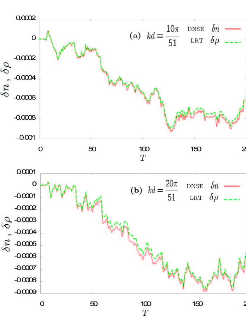
Figure 2: (Color online) Time evolution for the change of the density at the 10th site for (a) $kd=10\pi/51$ and (b) $kd=20\pi/51$ (region for real eigenvalues) with $T=\frac{Jt}{\hbar}$. The solid line represents the result of DNSE $\delta n_{10}(T)$ while the dashed line represents that of LRT $\langle\delta\hat{\rho}_{10}(T)\rangle$.

The critical value of $k$, giving a boundary between real and complex modes, is determined from $kd=\pi/2$. In Fig. 2, the time evolution of the changes of the density at the 10th site are plotted for (a) $kd=10\pi/51$ and (b) $kd=20\pi/51$, in both of the cases all the eigenvalues are real. We can see that the results of LRT fit that of DNSE with high precision, as is expected.

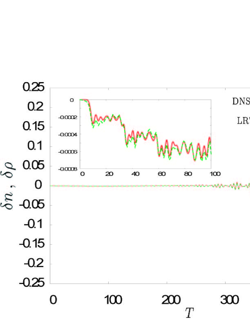
Figure 3: (Color online) Time evolution of the change of the density at the 10th site for $kd=26\pi/51$ (region for complex eigenvalues) with $T=Jt/\hbar$. The solid line represents the result of DNSE $\delta n_{10}(T)$ while the dashed line represents that of LRT $\langle\delta\hat{\rho}_{10}(T)\rangle$.

Move to the case in which complex modes appear. In Fig. 3, the time evolution fo the change of the density at the 10th site is plotted for $kd=26\pi/51$, this time the complex eigenvalues exist. One can find that the density response for small perturbation show the characteristic behavior. The change of density for $kd=26\pi/51$ are larger than that of $kd=10\pi/51$ or $kd=20\pi/51$ and grows exponentially. This behavior is caused by the complex eigenvalues. The result of LRT is in good agreement with that of DNSE again. Recall that the operators $\hat{A}_{\boldsymbol{k\bar{q}_{\rm c}}}$, $\hat{B}_{\boldsymbol{k\bar{q}_{\rm c}}}$ and the state $|0\rangle_{\oplus}$ are essential in our LRT formulation. The above agreement is not trivial at all when there are complex eigenmodes.

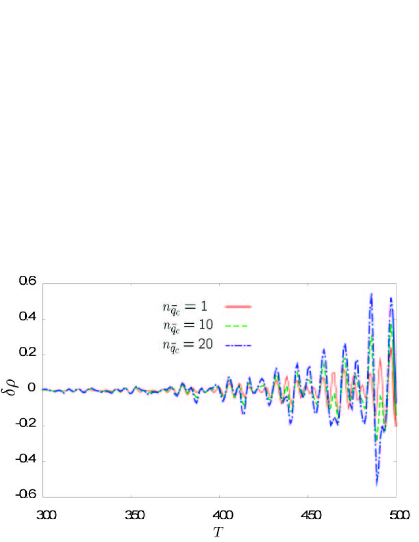
Figure 4: (Color online) Time evolution of the density at the 10th site $\langle\delta\hat{\rho}_{10}(T)\rangle$ with $T=Jt/\hbar$, calculated with the state defined in Eq. (212) for the interval between $T=300$ and $T=500$. The solid, dashed and dashed-dotted lines correspond to $n_{\bar{q}_{\rm c}}=1,10$ and $20$, respectively.

Next, we focus on one of the complex modes, characterized by the Bloch vector $\bar{q}_{\rm c}=2\pi/51$, and employ the following singly excited state for $|N_{\rm C}\rangle_{\oplus}$

$$|N_{\rm C}\rangle_{\oplus} = |0\cdots n_{\bar{q}_{\rm c}}\cdots 0\rangle_{\oplus}\,.$$ (212)

In Fig. 4, the quantity $\langle\delta\hat{\rho}_{10}(t)\rangle$ is plotted as a function of time. As $n_{\bar{q}_{\rm c}}$ increases, the amplitude of the response becomes larger and the exponentially diverging behavior becomes prominent. Thus it seems that the excitations of the complex modes hasten the collapse of condensates.

VII Summary

We have investigated the dynamical instability of Bose-Einstein condensation flowing in an optical lattice. The formulation in this paper is based on quantum field theory (QFT). The field operator must include complex modes for the dynamically unstable system, otherwise the canonical commutation relations would be violated.

We have attempted to diagonalize the unperturbed Hamiltonian under the tight-binding approximation, but it is not diagonalizable in the conventional bosonic representation. Nevertheless one can find its eigenstates, i.e., the vacuum and excited states in the complex mode sectors. Then, the physical state conditions (PSCs) were introduced to restrict the state space, so that we can start with the consistent stable particle in QFT.

As an application of our formulation to the problem of the dynamical instability, we consider the response of a condensate against external perturbation in the regime of the linear response theory (LRT). The numerical results of LRT with complex modes are to be compared with those from the discrete Schrödinger equation (DNSE). It is remarkable that both of the results coincide with each other although the two methods are quite different. The state $|0\rangle_{\oplus}$ and the operators $\hat{A}_{\boldsymbol{k\bar{q}_{\rm c}}}$ and $\hat{B}_{\boldsymbol{k\bar{q}_{\rm c}}}$ are crucial for our formulation of LRT. It is an interesting observation that the excited state in the complex mode sector hastens the collapse of the condensate in comparison with the vacuum state.

Appendix A Eigenfunctions of the Bogoliubov–de Gennes equation

In this Appendix, we rephrase the contents in Sec. IV from the viewpoint of the Bogoliubov-de Gennes (BdG) equation. The QFT formalism on the trapped BECs with vortices in Ref. MOSY is based on the BdG equation.

The relevant BdG equation is, in the doublet notation,

$$Tx_{n}(\boldsymbol{x})=\hbar\omega_{n}x_{n}(\boldsymbol{x})$$ (213)

where

$$T = \left(\begin{array}[]{cc}L&M\\ -M^{*}&-L\end{array}\right)\,,$$ (216)

$$x_{n}(\boldsymbol{x}) = \left(\begin{array}[]{c}f_{n}(\boldsymbol{x})\\ g_{n}(\boldsymbol{x})\end{array}\right)\,,$$ (219)

$$L = K+V_{\mathrm{opt}}-\mu+2g|v(\boldsymbol{x})|^{2}\,,$$ (220)

$$M = gv^{2}(\boldsymbol{x})\,.$$ (221)

The operator $T$ has the pseudo-Hermitian property of

$$\sigma_{3}T^{\dagger}\sigma_{3}=T\,$$ (222)

correspondingly to Eq. (63). This leads us to define the following inner product for an arbitrary pair of doublets,

$$(r,s) \equiv \int d^{3}x\,r^{\dagger}(\boldsymbol{x})\sigma_{3}s(\boldsymbol{x})$$ (223)

$$= \int\!d^{3}x\big{[}r_{1}^{*}(\boldsymbol{x})s_{1}(\boldsymbol{x})-r_{2}^{*}(\boldsymbol{x})s_{2}(\boldsymbol{x})\big{]},$$ (224)

where

$$r(\boldsymbol{x})=\left(\begin{array}[]{c}r_{1}(\boldsymbol{x})\\ r_{2}(\boldsymbol{x})\end{array}\right)\,,\qquad s(\boldsymbol{x})=\left(\begin{array}[]{c}s_{1}(\boldsymbol{x})\\ s_{2}(\boldsymbol{x})\end{array}\right)\,.$$ (229)

We may also define a (squared) “norm” of $r$ as $||r||^{2}\equiv(r,r)$, which is not positive-definite. One easily obtains

$$(\hbar\omega_{n}-\hbar\omega_{n^{\prime}}^{*})(x_{n^{\prime}},x_{n})=0.$$ (230)

As a counterpart of Eq. (66) we find the relation,

$$\sigma_{1}T^{*}\sigma_{1}=-T\,.$$ (231)

It turns out that for any eigenvector $x_{n}(\boldsymbol{x})$ whose eigenvalue is denoted by $\hbar\omega_{n}$ the doublet $y_{n}(\boldsymbol{x})=\sigma_{1}x_{n}^{*}(\boldsymbol{x})$ becomes an eigenvector with the eigenvalue $-\hbar\omega_{n}^{*}$.

When the eigenvalues are real, we have the following orthonormal relations, consistent with Eq. (230):

$$(x_{n^{\prime}},x_{n}) = \delta_{n^{\prime}n},$$ (232)

$$(y_{n^{\prime}},y_{n}) = -\delta_{n^{\prime}n},$$ (233)

$$(y_{n^{\prime}},x_{n}) = 0.$$ (234)

Complex modes appear in a pair for the BdG equation (213), i.e., any eigenstate $\zeta_{m}$ belonging to a complex eigenvalue $\hbar\omega_{m}$ is accompanied by another eigenstate $\eta_{\ell}$ whose eigenvalue $\hbar\omega_{\ell}$ is a complex conjugate of $\hbar\omega_{m}$, $\hbar\omega_{\ell}=\hbar\omega_{m}^{*}$. This fact is shown in constructing eigenstates explicitly in Sec. IV. The “norm” of the eigenstates of complex eigenvalues is zero,

$$\|\zeta_{m}\|^{2}=\|\eta_{\ell}\|^{2}=0\,,$$ (235)

since $(\hbar\omega_{m}-\hbar\omega_{m}^{*})$ is not zero in Eq. (230). The “zero norm” is a necessary condition for the emergence of complex eigenvalues. The pair of the eigenvectors $\zeta_{m}$ and $\eta_{\ell}$ are not orthogonal to each other in general,

$$(\eta_{\ell},\zeta_{m})\neq 0$$ (236)

as there is a vanishing factor of $(\hbar\omega_{m}-\hbar\omega_{\ell}^{*})$ on the left-hand side of Eq. (230).

Let us expand the field operator in the doublet notation in terms of the eigenfunctions of the BdG equation,

$$\hat{\Phi}(\boldsymbol{x},t) = \sum_{\boldsymbol{\bar{q}_{\rm r}}}\left[x_{\boldsymbol{k\bar{q}_{\rm r}}}(\boldsymbol{x})\hat{b}_{\boldsymbol{k\bar{q}_{\rm r}}}(t)+y_{\boldsymbol{k\bar{q}_{\rm r}}}(\boldsymbol{x})\hat{b}_{\boldsymbol{k\bar{q}_{\rm r}}}^{{\dagger}}(t)\right]$$

$${}+\sum_{\boldsymbol{\bar{q}_{\rm c}}}\left[\zeta_{\boldsymbol{k\bar{q}_{\rm r}}}(\boldsymbol{x})\hat{A}_{\boldsymbol{k\bar{q}_{\rm r}}}(t)+\eta_{\boldsymbol{k\bar{q}_{\rm r}}}(\boldsymbol{x})\hat{B}_{\boldsymbol{k\bar{q}_{\rm r}}}^{{\dagger}}(t)\right]\,,$$

where

$$\hat{\Phi}(\boldsymbol{x},t)=\left(\begin{array}[]{c}\hat{\phi}(\boldsymbol{x},t)\\ \hat{\phi}^{{\dagger}}(\boldsymbol{x},t)\end{array}\right)\,,$$ (240)

as in the case of a BEC with a vortex MOSY . Comparing this expansion with Eq. (137) and its Hermitian conjugate, we have

$$x_{\boldsymbol{k\bar{q}_{\rm r}}}(\boldsymbol{x}) = \left(\begin{array}[]{c}u_{\boldsymbol{k\bar{q}_{\rm r}}}f_{\boldsymbol{k\bar{q}_{\rm r}}}(\boldsymbol{x})\\ v_{\boldsymbol{k\bar{q}_{\rm r}}}f_{\boldsymbol{k-\bar{q}_{\rm r}}}^{*}(\boldsymbol{x})\end{array}\right)\,,$$ (243)

$$y_{\boldsymbol{k\bar{q}_{\rm r}}}(\boldsymbol{x}) = \left(\begin{array}[]{c}v_{\boldsymbol{k\bar{q}_{\rm r}}}f_{\boldsymbol{k\bar{q}_{\rm r}}}(\boldsymbol{x})\\ u_{\boldsymbol{k\bar{q}_{\rm r}}}f_{\boldsymbol{k}-\boldsymbol{\bar{q}_{\rm r}}}^{*}(\boldsymbol{x})\end{array}\right)\,,$$ (246)

$$\zeta_{\boldsymbol{k\bar{q}_{\rm c}}}(\boldsymbol{x}) = \left(\begin{array}[]{c}u_{\boldsymbol{k\bar{q}_{\rm c}}}f_{\boldsymbol{k\bar{q}_{\rm c}}}(\boldsymbol{x})\\ -iu^{*}_{\boldsymbol{k-\bar{q}_{\rm c}}}f_{\boldsymbol{k}-\boldsymbol{\bar{q}_{\rm c}}}^{*}(\boldsymbol{x})\end{array}\right)\,,$$ (249)

$$\eta_{\boldsymbol{k\bar{q}_{\rm c}}}(\boldsymbol{x}) = \left(\begin{array}[]{c}-iu^{*}_{\boldsymbol{k-\bar{q}_{\rm c}}}f_{\boldsymbol{k-\bar{q}_{\rm c}}}(\boldsymbol{x})\\ u_{\boldsymbol{k\bar{q}_{\rm c}}}f_{\boldsymbol{k}\boldsymbol{\bar{q}_{\rm c}}}^{*}(\boldsymbol{x})\end{array}\right).$$ (252)

It is straightforward to check the following orthonormal relations,

$$(x_{\boldsymbol{k\bar{q}_{\rm r}^{\prime}}},x_{\boldsymbol{k\bar{q}_{\rm r}}}) = \delta_{\boldsymbol{\bar{q}_{\rm r}\bar{q}_{\rm r}^{\prime}}}\,,$$ (253)

$$(y_{\boldsymbol{k\bar{q}_{\rm r}^{\prime}}},y_{\boldsymbol{k\bar{q}_{\rm r}}}) = -\delta_{\boldsymbol{\bar{q}_{\rm r}\bar{q}_{\rm r}^{\prime}}}\,,$$ (254)

$$(y_{\boldsymbol{k\bar{q}_{\rm r}^{\prime}}},x_{\boldsymbol{k\bar{q}_{\rm r}}}) = 0\,,$$ (255)

and

$$(\zeta_{\boldsymbol{k\bar{q}_{\rm c}^{\prime}}},\zeta_{\boldsymbol{k\bar{q}_{\rm c}}}) = 0\,,$$ (256)

$$(\eta_{\boldsymbol{k\bar{q}_{\rm c}^{\prime}}},\eta_{\boldsymbol{k\bar{q}_{\rm c}}}) = 0\,,$$ (257)

$$(\eta_{\boldsymbol{k\bar{q}_{\rm c}^{\prime}}},\zeta_{\boldsymbol{k\bar{q}_{\rm c}}}) = i\delta_{\boldsymbol{\bar{q}_{\rm c}\bar{q}_{\rm c}^{\prime}}}\,.$$ (258)

Appendix B Expression of Density Response

In this Appendix, we give the detailed expression of the density response $\langle\delta\hat{\rho}_{i}(t)\rangle$. The state by which the expectation $\langle\cdot\rangle$ is taken is found in Eq. (202). We restrict ourselves to the case of one dimension in space.

The external perturbation is given as

$$\delta V_{i}(t)=S\exp\left(\frac{x_{i}-I_{\rm s}d/2}{\sigma}\right)^{2}\theta(t-t_{0})\,.$$ (259)

Then the expression of the density response becomes

$$\langle\delta\hat{\rho}_{i}(t)\rangle=\langle\delta\hat{\rho}_{i}^{(0)}(t)\rangle+\langle\delta\hat{\rho}_{i}^{\rm(ex)}(t)\rangle\,,$$ (260)

where

$$\langle\delta\hat{\rho}_{i}^{(0)}(t)\rangle = \frac{2S}{\hbar I_{\rm s}}\sum_{j,\bar{q}}\exp\left(\frac{x_{j}-I_{\rm s}d/2}{\sigma}\right)^{2}\frac{n_{\rm c}(u_{k\bar{q}}+v_{k\bar{q}})^{2}}{\omega_{k\bar{q}}^{(+)}}\Big{[}\cos\left\{\bar{q}(x_{i}-x_{j})-\omega_{k\bar{q}}^{(+)}(t-t_{0})\right\}-\cos\{\bar{q}(x_{i}-x_{j})\}\Big{]}\,,$$

$$\langle\delta\hat{\rho}_{i}^{(\mathrm{ex})}(t)\rangle = \frac{2S}{\hbar I_{\rm s}}\sum_{j}\sum_{\bar{q}_{1},\bar{q}_{2}\neq 0}\exp\left(\frac{x_{j}-I_{s}d/2}{\sigma}\right)^{2}\big{\{}(n_{{\bar{q}}_{1}}+1)(n_{{-\bar{q}}_{2}}+1)-n_{{\bar{q}}_{1}}n_{{-\bar{q}}_{2}}\big{\}}$$ (262)

$$\times{\rm Re}\bigg{[}\frac{u_{k\bar{q}_{1}}v_{k\bar{q}_{2}}(u_{k\bar{q}_{1}}v_{k\bar{q}_{2}}+u_{kq_{2}}v_{kq_{1}})}{(\omega_{k\bar{q}_{1}}^{(+)}+\omega_{k-\bar{q}_{2}}^{(+)})I_{s}}\Big{\{}\cos\big{(}(\bar{q}_{1}-\bar{q}_{2})(x_{i}-x_{j})-(\omega_{k\bar{q}_{1}}^{(+)}+\omega_{k-\bar{q}_{2}}^{(+)})(t-t_{0})\big{)}$$

$$\hskip 170.71652pt{}-\cos\big{(}(\bar{q}_{1}-\bar{q}_{2})(x_{i}-x_{j})\big{)}\Big{\}}\bigg{]}\,.$$