Flat Möbius strips of given isotopy type in $\R^{3}$
whose centerlines are geodesics or
lines of curvature

Abstract.

We construct flat Möbius strips of arbitrary isotopy types, whose centerlines are geodesics or lines of curvature.

Introduction

Let $\varphi(p,t)=(-p,-t)$ ($|t|<1,\,\,p\in S^{1}$) be an involution on $S^{1}\times(-1,1)$, where

$$S^{1}:=\{p\in\R^{2}\,;\,|p|=1\}.$$

We denote by $\mathbb{M}$ the quotient of $S^{1}\times(-1,1)$ by the map $\varphi$, and denote by

$$\pi:S^{1}\times(-1,1)\to\mathbb{M}:=S^{1}\times(-1,1)/\sim_{\varphi}$$

the canonical projection. An embedding $f:\mathbb{M}\to\R^{3}$ is called a Möbius strip and the restriction of $f$ on the line $\{(p,t)\in S^{1}\times(-1,1)\,;\,t=0\}$ is called the centerline of the Möbius strip. A Möbius strip $f$ is called rectifying (or geodesic) if the centerline is a geodesic. On the other hand, a Möbius strip is called a Möbius developable if it is a ruled surface and its Gaussian curvature vanishes identically. It should be remarked that constructing a concrete example of Möbius developable is not so easy, and classical such examples are given in Wunderlich [W], Chiconne-Kalton [CK], Schwarz [S1, S2],and Randrup-Røgen [RR1].

A Möbius developable $f$ is called principal (or orthogonal) if the centerline is orthogonal to the asymptotic line. On the complement of the set of umbilics on $\mathbb{M}$, the centerline of the principal developable $f$ consists of a line of curvature. It should be remarked that any Möbius developable has at least one umbilcs (See Corollary 3.5 in [MU] and also Proposition 1.9 in Section 1.) In this paper, we shall prove the following two theorems:

Theorem A. There exists a principal real-analytic Möbius developable which is isotopic to a given Möbius strip.

It should be remarked that the first example of unknotted principal real-analytic Möbius developable was given in [CK].

Theorem B. There exists a rectifying real-analytic Möbius developable which is isotopic to a given Möbius strip.

When we ignore the property of the centerline, the existence of a $C^{\infty}$ Möbius developable with a given isotopy type has been shown: In fact, Chicone and Kalton showed (in 1984 see [CK]) that the existence of Möbius developable whose center line is an arbitrary given generic space curves. After that, Røgen [R] showed that any embedded surfaces with boundary in $\R^{3}$ can be isotopic to flat surfaces.

If we expand a flat Möbius developable into their asymptotic directions, then we get a flat surface whose asymptotic lines are all complete, and such a surface may have singular points in general. In [MU], the global properties of such surfaces are investigated.

As a point of view from paper-handicraft, we know experimentally the existence of a developable Möbius strip which can be given as an isometric deformation of a rectangular domain on a plane. Such a Möbius strip must be rectifying, since the property that the centerline is a geodesic is preserved by the isometric deformation. On the other hand, any rectifying Möbius developable can be obtained by an isometric deformation of a rectangular domain on a plane (See Proposition 1.14). Thus, Theorem B implies that one can construct a developable Möbius strip of given isotopy type via a rectangular ribbon.

1. Preliminaries

Let $I:=[a,b]$ be a closed interval, and $\gamma(t)$ ($a\leq t\leq b$) a regular space curve. Then the function

$$\kappa(t):=\frac{|\dot{\gamma}(t)\times\ddot{\gamma}(t)|}{|\dot{\gamma}(t)|^{3}}$$

is called the curvature function of $\gamma$. A point where $\kappa(t)$ vanishes is called an inflection point of $\gamma$, where $\dot{\gamma}=d\gamma/dt$.

Let $\xi(t)$ be a vector field in $\R^{3}$ along the curve $\gamma(t)$. We set

$$F_{\gamma,\xi}(t,u):=\gamma(t)+u\xi(t)\qquad(t\in I,\,\,|u|<\varepsilon),$$

where $\varepsilon$ is a sufficiently small positive constant. Then $F_{\gamma,\xi}$ is called a ruled strip if it satisfies

$$\dot{\gamma}(t)\times\xi(t)\neq 0,$$

where $\times$ is the vector product in $\R^{3}$. In this case, $F_{\gamma,\xi}$ gives an immersion for sufficiently small $\varepsilon$. Moreover, if it satisfies

(1.1) $$\operatorname{det}(\dot{\gamma}(t),\xi(t),\dot{\xi}(t))=0\qquad(a\leq t\leq b),$$

then $F_{\gamma,\xi}$ is called a developable strip. In fact, it is well-known that (1.1) is equivalent to the condition that the Gaussian curvature of $F_{\gamma,\xi}$ vanishes identically.

Definition 1.1.

Let $F_{\gamma,\xi}$ be a developable strip. Then it is called principal or orthogonal if it satisfies

(1.2) $$\xi(t)\cdot\dot{\gamma}(t)=0\qquad(a\leq t\leq b),$$

where $\cdot$ means the canonical inner product in $\R^{3}$. In fact, the condition (1.2) is the orthogonality of the centerline with respect to the asymptotic direction. If $\gamma(t)$ is not an umbilic, the centerline is a line of curvature near $\gamma(t)$.

The following assertion can be proved directly:

Proposition 1.2.

Let $\gamma$ be a regular space curve, and $\xi(t)$ a vector field along $\gamma(t)$ such that

(1.3) $$\xi(t)\cdot\dot{\gamma}(t)=0,\qquad\dot{\xi}(t)\times\dot{\gamma}(t)=0\qquad(a\leq t\leq b).$$

Then $F_{\gamma,\xi}$ gives a principal developable strip.

Remark 1.3.

One can prove that any principal developable strip is given in this manner.

Remark 1.4.

The condition (1.3) means that $\xi(t)$ is parallel with respect to the normal connection. In particular, the length $|\xi(t)|$ is constant along $\gamma$. When $\gamma$ does not admit inflection points, the torsion function of $\gamma$ is defined by

$$\tau(t):=\frac{\operatorname{det}(\dot{\gamma}(t),\ddot{\gamma}(t),\dddot{\gamma}(t))}{|\dot{\gamma}(t)\times\ddot{\gamma}(t)|^{2}}.$$

We now take $t$ to be the arclength parameter. Then, as pointed out in [CK],

$$P_{0}(t):=\left(\sin\int_{a}^{t}\tau(s)ds\right){\mathbf{n}}(t)+\left(\cos\int_{a}^{t}\tau(s)ds\right){\mathbf{b}}(t)$$

gives a parallel vector field on the normal bundle $T^{\perp}_{\gamma}$ of $\gamma$, that is, $\dot{P}_{0}(t)$ is proportional to $\dot{\gamma}(t)$. (Here ${\mathbf{n}}(t)$ and ${\mathbf{b}}(t)$ are the principal normal vector field and the bi-normal vector field of $\gamma(t)$, respectively.) It can be easily checked that any parallel vector field satisfying (1.3) is expressed by

$$P(t):=(\cos\delta)P_{0}(t)+(\sin\delta)\biggl{(}\dot{\gamma}(t)\times P_{0}(t)\biggr{)},$$

for a suitable constant $\delta\in[a,b)$. Let $\xi(t)$ ($a\leq t\leq b$) be a non-vanishing normal vector field along $\gamma$, that is, it satisfies $\xi(t)\cdot\dot{\gamma}=0$. Let $\alpha(t)$ be the leftward angle of $\xi(t)$ from $P(t)$. We set

$$\operatorname{Tw}_{\gamma}(\xi):=\alpha(b)-\alpha(a)$$

which is called the total twist of $\xi$ along $\gamma$, and is equal to the total change of angles of $\xi(t)$ towards the clockwise direction with respect to $P_{0}(t)$. When $|\xi(t)|=1$, it is well known that the following identity holds:

(1.4) $$\operatorname{Tw}_{\gamma}(\xi)=\frac{1}{2\pi}\int_{a}^{b}\operatorname{det}(\dot{\gamma}(t),\xi(t),\dot{\xi}(t))\,dt.$$

Definition 1.5.

Let $F_{\gamma,\xi}$ be a developable strip. Then it is called rectifying (or geodesic) if it satisfies

$$\dot{\xi}(t)\cdot\ddot{\gamma}(t)=0\qquad(a\leq t\leq b),$$

where $\cdot$ means the canonical inner product in $\R^{3}$.

First, we give a trivial (but important) example:

Example 1.6.

(The cylindrical strips) Let $\gamma(t)={}^{t}(x(t),y(t),0)$ be a regular curve which lies entirely in the $xy$-plane. Then the cylinder

$$F(t,u):=\gamma(t)+{\begin{pmatrix}0\\ 0\\ u\end{pmatrix}}$$

over $\gamma$ gives a developable strip which is principal and rectifying at the same time. It is called a cylindrical strip.

Again, we return to the general setting: Let $\gamma(t)$ ($a\leq t\leq b$) be a regular space curve. If the torsion function $\tau(t)$ of $\gamma(t)$ does not vanish, then the rectifying developable over $\gamma$ is uniquely determined as follows: We set

$$D(t)=\frac{\tau(t)}{\kappa(t)}{\mathbf{t}}(t)+{\mathbf{b}}(t),$$

which is called the normalized Darboux vector field (cf. Izumiya-Takeuchi [IT]), where ${\mathbf{t}}(t):=\dot{\gamma}(t)/|\dot{\gamma}(t)|$. The original Darboux vector field is equal to ${\mathbf{n}}(t)\times\dot{{\mathbf{n}}}(t)$, which is proportional to $D(t)$, where ${\mathbf{t}}(t),{\mathbf{n}}(t),{\mathbf{b}}(t)$ are the unit tangent vector, the unit principal normal vector and the unit bi-normal vector, respectively.

Then one can easily get the following assertion:

Proposition 1.7.

Let $\gamma(t)$ be a regular space curve without inflection points, and $D(t)$ the normalized Darboux vector field along $\gamma$. Then $F_{\gamma,D}$ gives a rectifying developable strip.

Remark 1.8.

One can prove that any rectifying developable strip is given in this manner.

Let $F_{\gamma,\xi}$ be a developable strip over a regular space curve $\gamma(t)$ ($a\leq t\leq b$). If it holds that

$$\gamma^{(n)}(a)=\gamma^{(n)}(b)\qquad(n=0,1,2,...)$$

then $\gamma$ gives a smooth closed curve, where $\gamma^{(n)}(t):=d^{n}\gamma/dt^{n}$. Moreover, if

(1.5) $$\xi^{(n)}(a)=-\xi^{(n)}(b)\qquad(n=0,1,2,...)$$

holds, then $F_{\gamma,\xi}$ gives a Möbius developable as defined in Introduction. We denote by the boundary of $F_{\gamma,\xi}$ by $B_{\gamma}$. The half of the linking number

$$\operatorname{Mtn}(F_{\gamma,\xi}):=\frac{1}{2}\operatorname{Link}(\gamma,B_{\gamma})$$

is called the Möbius twisting number, which takes values in $\pm\frac{1}{2},\pm\frac{3}{2},\pm\frac{5}{2},\cdots$ (cf. [R, Definition 3]). Here $\operatorname{Mtn}(F_{\gamma,\xi})=(2n+1)/2$ implies that the strip is $(2n+1)\pi$-twisted into clockwise direction. Let ${\mathbf{c}}$ be a unit vector in $\R^{3}$ and suppose that the projection of the centerline $\gamma$ into the plane $P_{\mathbf{c}}$ perpendicular to ${\mathbf{c}}$ gives a generic plane curve. Then we get a knot diagram of $\gamma$ on the plane $P_{\mathbf{c}}$, and its writhe $\operatorname{Wr}_{{\mathbf{c}}}(\gamma)$ is defined, which is the total sum of the sign of crossings on the knot diagram. Then the following identity is well-known:

(1.6) $$\operatorname{Mtn}(F_{\gamma,\xi})=-\operatorname{Tw}_{\gamma}(\xi^{\perp})+\operatorname{Tw}_{\gamma}({\mathbf{c}}^{\perp})+\operatorname{Wr}_{{\mathbf{c}}}(\gamma),$$

where $\xi^{\perp}$ and ${\mathbf{c}}^{\perp}$ mean the projection of vectors $\xi(t),{\mathbf{c}}$ into the normal plane $T^{\perp}_{\gamma}$ at $\gamma(t)$.

Here, we shall recall the following result:

Proposition 1.9.

([MU, Corollary 3.5]) Any Möbius developable admits at least one umbilical point.

Proof.

For the sake of convenience, we shall give here a proof. Let $\gamma(t)$ ($a\leq t\leq b$) be the centerline of the Möbius developable. We may regard $\gamma(t)$ is a $c$-periodic regular space curve ($c=b-a$), that is

$$\gamma(t+c)=\gamma(t)\qquad(t\in\R).$$

Then the Möbius developable can be written as

$$F(t,u)=\gamma(t)+u\xi(t)\qquad(|u|<\varepsilon),$$

where $\xi(t)$ is a unit vector field along $\gamma$ such that

(1.7) $$\xi(t+c)=-\xi(t)\qquad(t\in\R).$$

Let $\nu(t)$ be the unit normal vector field of $F(t,u)$, which depends only on $t$. Suppose that $f$ has no umbilics. Then we can take a local curvature line coordinate $(x,y)$. Then by the Weingarten formula, we have

(1.8) $$\nu_{x}=-\lambda_{1}f_{x},\qquad\nu_{y}=-\lambda_{2}f_{y},$$

where $\lambda_{1},\lambda_{2}$ are principal curvatures. Without loss of generality, we may assume that $\lambda_{1}=0$. Then $f_{x}(t,u)$ is proportional to $\xi(t)$. Since $\lambda_{1}=0$, (1.8) yields that

(1.9) $$\dot{\nu}(t)=\nu_{x}\dot{x}+\nu_{y}\dot{y}=\nu_{y}\dot{y}=\dot{y}\lambda_{2}f_{y},$$

namely, $\dot{\nu}$ is proportional to the non-zero principal direction $f_{y}$. Since the two principal directions are orthogonal, $\xi(t)$ must be orthogonal to $\nu(t)$ and $\dot{\nu}(t)$. Since we have assumed that $f$ has no umbilical point, $\nu(t)\times\dot{\nu}(t)$ never vanishes for all $t$. Thus, we can write

(1.10) $$\xi(t)=a(t)\nu(t)\times\dot{\nu}(t),$$

where $a(t)$ is a smooth function. Since $f$ is non-orientable, $\nu(t)$ is odd-periodic (that is $\nu(t+c)=-\nu(t)$). In particular, $\nu(t)\times\dot{\nu}(t)$ must be $c$-periodic, that is

(1.11) $$\nu(t+c)\times\dot{\nu}(t+c)=\nu(t)\times\dot{\nu}(t)\qquad(t\in\R).$$

By (1.7), (1.10) and (1.11), the function $a(t)$ must satisfy the property $a(t+c)=-a(t)$. In particular, there exists $t_{0}\in[a,b)$ such that $a(t_{0})=0$. Thus we have $\xi(t_{0})=0$, which contradicts that $\xi$ is a unit vector field. q.e.d.

Now, we would like to recall a method for constructing real analytic rectifying Möbius developables from [RR1]. We now assume that $\gamma(t)$ $(a\leq t\leq b)$ gives an embedded closed real analytic regular space curve, which has no inflection points on $(a,b)$. Since a rectifying Möbius developable must have at least one inflection point (See [RR1]), $t=a$ must be the inflection point of $\gamma$. Let $D(t)$ ($a<t<b$) be the normalized Darboux vector field of $\gamma$. Then $F_{\gamma,D}$ gives a rectifying Möbius developable if and only if $\xi:=D$ satisfies (1.5), which reduces to the following Lemma 1.10: The first non-vanishing non-zero coefficient vector ${\mathbf{c}}(\neq 0)$ of the expansion of $\dot{\gamma}(t)\times\ddot{\gamma}(t)$ at $t=a$ satisfies

$$\dot{\gamma}(t)\times\ddot{\gamma}(t)={\mathbf{c}}(t-a)^{N}+\mbox{higher order terms},$$

where the integer $N(\geq 1)$ is called the order of the inflection point and the point $t=a$ is called a generic inflection point. (The number $N$ is independent of the choice of the parameter $t$ of the curve.) Next we set

$$\Delta(t):=\operatorname{det}(\dot{\gamma}(t),\ddot{\gamma}(t),\dddot{\gamma}(t)),$$

which is the numerator in the definition of the torsion function. (See Remark 1.4.) Then there exists a nonzero constant $c_{1}$ such that

$$\Delta(t)=c_{1}(t-a)^{M}+\mbox{higher order terms},$$

where the integer $M(\geq 1)$ is called the order of torsion at $t=0$. The following assertion is very useful:

Lemma 1.10.

(Randrup-Røgen [RR]) Let $\gamma(t)$ $(a\leq t\leq b)$ be a closed regular space such that $t=a$ is an inflection point, and there are no other inflection point on $(a,b)$. Then the normalized Darboux vector field $D(t)$ can be smoothly extended as a $C^{\infty}$-vector field around $t=a$ if and only if $M/N\geq 3$. In this case, $F_{\gamma,D}$ defines a rectifying developable. Moreover, if $N$ is odd, $F_{\gamma,D}$ is non-orientable.

As a corollary, we prove the following assertion, which will play an important role in Section 3.

Corollary 1.11.

Suppose that the inflection point at $t=a$ is generic $($that is, $N=1)$. Then $F_{\gamma,D}$ gives a rectifying Möbius developable if and only if

$$\operatorname{det}(\dot{\gamma}(t),\gamma^{(3)}(t),\gamma^{(4)}(t))$$

vanishes at $t=a$.

Proof.

Since $t=a$ is an inflection point, we have $\ddot{\gamma}(a)=0$. In particular,

$$\dot{\Delta}(t)=\operatorname{det}(\dot{\gamma}(t),\ddot{\gamma}(t),\gamma^{(4)}(t))$$

vanishes at $t=a$. On the other hand, we have

$$\ddot{\Delta}(a)=\operatorname{det}(\dot{\gamma}(a),\gamma^{(3)}(a),\gamma^{(4)}(a)),$$

which vanishes if and only if $M\geq 3$. q.e.d.

Here, we give a few examples.

Example 1.12.

(Wunderlich [W]) Consider a regular space curve

$$\gamma(t)=\frac{1}{\delta(t)}{\begin{pmatrix}3t+2t^{3}+t^{5}\\ 4t+2t^{3}\\ -24/5\end{pmatrix}}\qquad(t\in\R),$$

where $\delta(t)=9+4t^{2}+4t^{4}+t^{6}$. Then $\gamma(t)$ has no inflection point for $t\in\R$. Moreover, it can be smoothly extended as an embedding in $\R^{3}$. In fact,

$$\gamma(1/s)=\frac{1}{\hat{\delta}(s)}{\begin{pmatrix}3s^{5}+2s^{3}+s\\ 4s^{5}+2s^{3}\\ -24s^{6}/5\end{pmatrix}}\qquad(\hat{\delta}(s):=9s^{6}+4s^{4}+4s^{2}+1)$$

is smooth at $s=0$. This point $s=0$ is a generic inflection point with $N=1$ and $M=4$, and the induced rectifying Möbius developable is unknotted and of Möbius twisting number $1/2$. See Figure 1 left.

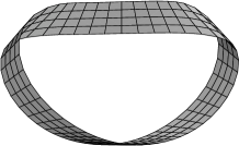
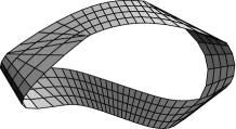
Figure 1. The Möbius strips given in Examples 1.12 and 1.13.

Next, we shall give a new example of a rectifying Möbius developable whose centerline has a non-generic inflection point.

Example 1.13.

Consider a regular space curve

$$\gamma(t)=\frac{1}{\delta(t)}{\begin{pmatrix}t^{9}+t^{7}+t^{5}+t^{3}+t\\ t^{5}+t^{3}+t\\ 1\end{pmatrix}}\qquad(t\in\R),$$

where $\delta(t):=t^{10}+t^{8}+t^{6}+t^{4}+t^{2}+1$. Like as in the previous example, $\gamma(1/s)$ is also real analytic at $s=0$ and $\gamma$ gives an embedded closed space curve in $\R^{3}$. Moreover, $s=0$ is an inflection point with $(N,M)=(3,10)$, that is, it is not a generic inflection point. By Lemma 1.10, the curve induces a real analytic Möbius developable which is unknotted and of Möbius twisting number $1/2$. See Figure 1 right.

Randrup-Røgen [RR1] gave other examples of rectifying Möbius developable via Fourier polynomials.

As pointed out in the introduction, any Möbius developable constructed from an isometric deformation of rectangular domain on a plane is rectifying. Conversely, we can prove the following, namely, any Möbius developable is an isometric deformation of rectangular domain on a plane:

Proposition 1.14.

Let $F=F_{\gamma,D}:[a,b]\times(\varepsilon,\varepsilon)$ be an $($embedded$)$ rectifying Möbius developable. Then there exists a point $t_{0}\in[a,b)$ such that the asymptotic direction $\xi(t_{0})$ at $f(t_{0},0)$ is perpendicular to $\dot{\gamma}(t_{0})$. In particular, the image $\{f(t,u)\in\R^{3}\,;\,t\neq t_{0}\}$ contains a subset which is isometric to a rectangular domain in a plane.

Proof.

Since $f$ is non-orientable, the unit asymptotic vector filed $\xi(t)$ is odd-periodic, that is, $\xi(a)=-\xi(b)$. Then we have

$$\xi(0)\cdot\dot{\gamma}(0)=-\xi(\pi)\cdot\dot{\gamma}(\pi),$$

which implies that the function $t\mapsto\xi(t)\cdot\dot{\gamma}(t)$ changes sign on $[a,b)$. By the intermediate vale theorem, there exists a point $t_{0}\in[0,\pi)$ such that

$$\xi(t_{0})\cdot\dot{\gamma}(t_{0})=0,$$

which proves the assertion. q.e.d.

2. A $C^{\infty}$ Möbius developable of a given isotopy-type

In this section, we construct a rectifying $C^{\infty}$ Möbius developable of a given isotopy-type. To accomplish this, we prepare a special kind of developable strip as follows:

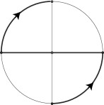
$\Longrightarrow$    

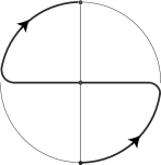
Figure 2. The original arc $\sigma$ (left) and $\hat{\sigma}$ (right)

(The twisting arcs) Let $S^{2}_{+}$ (resp. $S^{2}_{-}$) be an upper (resp. a lower) open hemisphere of the unit sphere, and let

$$\pi_{\pm}:S^{2}_{\pm}\to\bar{\Delta}^{2}:=\biggl{\{}(x,y)\in\R^{2}\,;\,x^{2}+y^{2}\leq 1\biggr{\}}$$

be two canonical orthogonal projections. Consider an oriented (piece-wise smooth) planar curve $\sigma$ on the closed unit disc $\bar{\Delta}^{2}$ as in Figure 2. Let $\hat{\sigma}$ be a $C^{\infty}$-regular curve rounding corner as in right-hand side of Figure 2. Then the oriented space curves as the inverse images

$$\tilde{\sigma}_{+}:=\pi_{+}^{-1}(\hat{\sigma}),\qquad\tilde{\sigma}_{-}:=\pi_{-}^{-1}(\hat{\sigma})$$

are called the leftward twisting arc or the rightward twisting arc, respectively. (See Figure 2.)

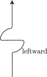
$\Longrightarrow$                            $\Longrightarrow$    

Figure 3. The marker of the insertion of a leftward (resp. rightward) twisting arc

From now on, we would like to twist a given planar curve by replacing a sufficiently small subarc with the above two twisting arcs. Namely, one can attach the leftward (resp. rightward) twisting arc into a given planar curve, and get a space curve. For the sake of simplicity, we indicate these two surgeries constructing space curves from a given planar curve symbolically as in Figure 3 left (resp. right).

If we connect two end points of a twisting arc by a planar arc in $xy$-plane, we get a closed curve. Since the curvature function (as a plane curve) of a twisting arc near the two end points as a plane curve takes opposite sign, the resulting closed curve has at least one inflection point. We need such an operation to construct several Möbius developables in later. The existence of inflection points is really needed for constructing rectifying Möbius strips. The following assertion is useful for counting Möbius twisting number of our latter examples:

Proposition 2.1.

Let $\tilde{\sigma}_{+}(t)$ and $\tilde{\sigma}_{-}(t)$ $(a\leq t\leq b)$ be the leftward and rightward twisting arcs parameterizing the set $\pi_{+}^{-1}(\hat{\sigma})$ $($resp. $\pi_{-}^{-1}(\hat{\sigma}))$ respectively. Then the space curves $\tilde{\sigma}_{\pm}(t)$ have no inflection points. Moreover, it holds that

(2.1) $$\operatorname{Tw}_{\tilde{\sigma}_{+}}(D_{+}^{\perp})-\operatorname{Tw}_{\tilde{\sigma}_{+}}({\mathbf{e}}_{3}^{\perp})=\pi,\qquad\operatorname{Tw}_{\tilde{\sigma}_{-}}(D_{-}^{\perp})-\operatorname{Tw}_{\tilde{\sigma}_{-}}({\mathbf{e}}_{3}^{\perp})=-\pi,$$

(2.2) $$\operatorname{Tw}_{\tilde{\sigma}_{+}}(\eta_{+})-\operatorname{Tw}_{\tilde{\sigma}_{+}}({\mathbf{e}}_{3}^{\perp})=\pi,\qquad\operatorname{Tw}_{\tilde{\sigma}_{-}}(\eta_{-})-\operatorname{Tw}_{\tilde{\sigma}_{-}}({\mathbf{e}}_{3}^{\perp})=-\pi,$$

where $D_{\pm}(t)$ is the Darboux vector field of $\tilde{\sigma}_{\pm}(t)$, ${\mathbf{e}}_{3}={}^{t}\!(0,0,1)$ and

$$\eta_{\pm}(t):=\tilde{\sigma}_{\pm}(t)\times\dot{\tilde{\sigma}}_{\pm}(t)$$

is the (leftward) unit co-normal vector of $\tilde{\sigma}$ on the unit sphere $S^{2}$. $($Here the normal sections $D_{\pm}^{\perp},{\mathbf{e}}_{3}^{\perp}$ with respect to ${\tilde{\sigma}}_{\pm}$ are obtained as the normal parts of the vectors $D_{\pm},{\mathbf{e}}_{3}$. See (1.6). $)$

Proof.

It is sufficient to prove the case of leftward twisting arc. Let ${\mathbf{b}}(t)$ be the bi-normal vector of $\tilde{\sigma}_{+}$ as a space curve. Since $\tilde{\sigma}_{+}$ is a curve on the unit sphere, the principal normal direction ${\mathbf{n}}(t)$ must be $-\sigma_{+}(t)$, and thus

$${\mathbf{b}}(t)={\mathbf{t}}(t)\times{\mathbf{n}}(t)=\tilde{\sigma}_{+}(t)\times{\mathbf{t}}(t)=\eta_{+}(t),$$

where ${\mathbf{t}}(t):=\dot{\gamma}(t)/|\dot{\gamma}(t)|$. Moreover, by the definition of the normalized Darboux vector field $D_{+}(t)$, we have

$$D^{\perp}_{+}(t)={\mathbf{b}}(t)=\eta_{+}(t).$$

Thus the first formula reduces to the second one.
Let $\theta(t)$ be the smooth function which gives the leftward angle of $\eta_{+}(t)$ from ${\mathbf{e}}_{3}^{\perp}$. Then, we have

$$\operatorname{Tw}_{\tilde{\sigma}_{+}}(\eta_{+})-\operatorname{Tw}_{\tilde{\sigma}_{+}}({\mathbf{e}}_{3}^{\perp})=\theta(1)-\theta(0).$$

Let ${\mathbf{t}}(t)$ be the unit tangent vector of $\tilde{\sigma}_{+}$ as a space curve. Then by definition of $\tilde{\sigma}_{+}$, we have

$${\mathbf{t}}(0)={\mathbf{t}}(1),\qquad{\mathbf{n}}(0)=-{\mathbf{n}}(1)$$

which yield

(2.3) $$\eta_{+}(0)={\mathbf{b}}(0)={\mathbf{t}}(0)\times{\mathbf{n}}(0)=-{\mathbf{t}}(1)\times{\mathbf{n}}(1)=-{\mathbf{b}}(1)=-\eta_{+}(1).$$

On the other hands, $\tilde{\sigma}_{+}(t)$ lies in $xy$-plane near $t=a,b$, the vector $\eta_{+}(t)={\mathbf{b}}(t)$ is proportional to ${\mathbf{e}}_{3}$ there. Thus we have that

$$\theta(1)-\theta(0)=\pi\,\,\mod 2\pi\boldsymbol{Z}.$$

Since we can easily check that $\theta(t)\geq 0$, we get $\theta(1)-\theta(0)=\pi$, which proves (2.2). q.e.d.

Lemma 2.2.

Let $\gamma(t)$ be a spherical curve parametrized by the arclength parameter. Then the leftward conormal vector field

$$\eta(t):=\gamma(t)\times\dot{\gamma}(t)$$

is parallel with respect the normal connection of $\gamma(t)$. In particular, $F_{\gamma,\eta}(t,u)$ is a principal developable strip.

Proof.

A normal vector field $\xi(t)$ along $\gamma$ is parallel with respect to the normal connection if and only if $\dot{\xi}(t)$ is proportional to $\dot{\gamma}$. Applying the Frenet formula, we have

$$\dot{\eta}(t)=\gamma(t)\times\ddot{\gamma}(t)=\kappa(t)\gamma(t)\times{\mathbf{n}}(t),$$

where ${\mathbf{n}}(t)$ and $\kappa(t)$ is the principal normal vector and the curvature function of $\gamma(t)$ as a space curve. Since $\gamma$ and ${\mathbf{n}}$ are both perpendicular to $\dot{\gamma}$, the vector $\gamma\times{\mathbf{n}}$ is proportional to $\dot{\gamma}$, which proves the assertion. q.e.d.

Definition 2.3.

Let $\tilde{\sigma}_{+}(t)$(resp. $\tilde{\sigma}_{-}(t)$) be the leftward (resp. rightward) twisting arc as in Proposition 2.1. Then

$$F^{\pm}_{p}(t,u):=\tilde{\sigma}_{\pm}(t)+u\eta_{\pm}(t)\qquad(\eta_{\pm}(t):=\tilde{\sigma}_{\pm}(t)\times\dot{\tilde{\sigma}}_{\pm}(t))$$

is called the principal twisting strip and

$$F^{\pm}_{g}(t,u):=\tilde{\sigma}_{\pm}(t)+uD_{\pm}(t)$$

is called the rectifying twisting strip, where $D_{\pm}(t)$ is the normalized Darboux field of $\tilde{\sigma}_{\pm}$.

By Proposition 2.1 and Lemma 2.2, $F^{\pm}_{p}$ is a principal developable satisfying (2.2), and $F^{\pm}_{g}$ is a rectifying developable satisfying (2.1).

$\Longrightarrow$         

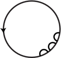
Figure 4. The construction of $C_{2m+1}$ via $C$.

Theorem 2.4.

For an arbitrarily given isotopy type of Möbius strip, there exists a $C^{\infty}$ principal $($resp. rectifying$)$ Möbius developable in the same isotopy class.

Proof.

First, we construct an unknotted principal Möbius developable of a given Möbius twisting number from a circle: Consider a circle $C$ in the $xy$-plane. We insert $2m+1$ leftward (resp. rightward) twisting arcs into $C$ and denote it by $C_{2m+1}$ or $C_{-2m-1}$ (See Figure 4.). If we build $2m+1$ principal twisting strips (each of which is congruent to $F^{\pm}_{p}$) on these twisting arcs, then we get a principal $C^{\infty}$ Möbius developable $F_{2m+1}$ whose centerline is $C_{2m+1}$. (Let $\gamma(t)$ ($a\leq t\leq b$) be a parametrization of centerline of $F_{2m+1}$. Then we can write

$$F_{2m+1}(t,u)=\gamma(t)+uP(t)\qquad(a\leq t\leq b,\,\,|u|<\varepsilon).$$

The image of the center line $\gamma(t)$ is a union of $m$ planar arcs and $m$ twisting arcs. On each planar arcs $P(t)$ is equal to ${\mathbf{e}}_{3}={}^{t}\!(0,0,1)$. On the other hand, $P(t)$ coincides with the co-normal vector on each twisting arc as a spherical curve. Since the twisting arc is planar near two end points, $P(t)$ is smooth at each end points of twisting arcs. Consequently, $P(t)$ satisfies the condition of Proposition 1.2 such that $P(a)=-P(b)$.) By (1.6) and (2.2), the Möbius twisting number of $F_{2m+1}$ is equal to $-(2m+1)/2$ (resp. $(2m+1)/2$) if we insert the leftward (resp. rightward) twisting strips.

Instead of principal twisting strips, we can insert rectifying twisting strips $F^{\pm}_{g}$ into $C_{2m+1}$. Then by (1.6) and (2.1), we also get a rectifying $C^{\infty}$ Möbius developable with the Möbius twisting number $\pm(2m+1)/2$.

Next, we construct a knotted principal Möbius developable of a given Möbius twisting number via a knot diagram. It should be remarked that the isotopy type of the given embedded Möbius strip is determined by its Möbius twisting number and the knot type of its centerline. (See [RR2].) Let $\gamma$ be the planar curve corresponding to the diagram. We replace every crossing of $\gamma$ by a pair of leftward and rightward twisting arcs as in Figure 5 (right). For the sake of simplicity, we indicate this operation as in Figure 6. When we will accomplish to construct the associated Möbius developable, this operation as in Figure 5 does not effect the Möbius twisting number, since the signs of the two twisting arcs are opposite.

$\Longrightarrow$    

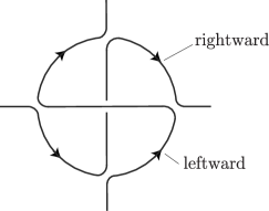
Figure 5. The crossing with the pair of twisting arcs

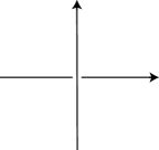
$\Longrightarrow$    

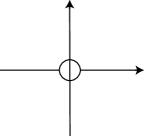
Figure 6. The marker of the pair of twisting arcs at a crossing

For example, letting $K$ be a knot diagram $3_{1}$ of the trefoil knot as in Figure 7 left, we replace each crossing by a pair of leftward and rightward twisting arcs (as in Figure 5 and Figure 6), and insert $2m+1$ leftward (resp. rightward) twisting arcs as in Figure 7 right. Then we get an embedded closed space curve $C^{K}_{2m+1}$ ($m\in\boldsymbol{Z}$) which is isotopic to the knot $K$. If we build principal twisting strips on all of the twisting arcs we inserted, then we get a principal $C^{\infty}$ Möbius developable $F^{K}_{2m+1}$. Since all crossing of $3_{1}$ are positive, the writhe is $3$, and thus the formula (1.6) and (2.2) yields that the Möbius twisting number of $F^{K}_{2m+1}$ is $3\mp(2m+1)/2$. Since $m$ is an arbitrary non-negative integer, we prove the existence of principal Möbius strip for the case of trefoil knot.

Similarly, we can prove the existence of principal Möbius strip $F^{K}_{2m+1}$ with an arbitrary Möbius twisting number for an arbitrary given knot diagram $K$.

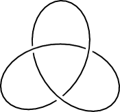
$\Longrightarrow$    

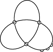
Figure 7. The construction of a Möbius developable via the knot diagram of $3_{1}$

Instead of the principal twisting strips, we can insert the rectifying twisting strips (cf. Definition 2.3). Then we also get a rectifying $C^{\infty}$ Möbius developable with an arbitrary isotopy type at the same time. q.e.d.

(Properties of asymptotic completion of Möbius strips)
Let $M^{2}$ be a $2$-manifold and $f:M^{2}\to\mathbf{R}^{3}$ a $C^{\infty}$-map. A point $p\in M^{2}$ is called regular if $f$ is an immersion on a sufficiently small neighborhood of $p$, and is called singular if it is not regular. Moreover, $f:M^{2}\to\mathbf{R}^{3}$ is called a (wave) front if

1. there exists a unit vector field $\nu$ along $f$ such that $\nu$ is perpendicular to the image of tangent spaces $f_{*}(TM)$. ( $\nu$ is called the unit normal vector field of $f$, which can be identified with the Gauss map $\nu:M^{2}\to\mathbf{R}^{3}$. )

2. The pair of maps

   $$L:=(f,\nu):M^{2}\to\mathbf{R}^{3}\times S^{2}(\cong T^{*}_{1}\mathbf{R}^{3})$$

   gives an immersion.

On the other hand, a smooth map $f:M^{2}\to\mathbf{R}^{3}$ is called a p-front if it is locally a front, that is, for each $q\in M^{2}$, there exists an open neighborhood $U_{q}$ such that the restriction $f|_{U_{q}}$ gives a front. By definition, a front is a p-front. A p-front is a front if and only if it has globally defined unit normal vector fields (namely, it is co-orientable).

Definition 2.5.

([MU])  The first fundamental form $ds^{2}$ of a flat p-front $f:M^{2}\to\R^{3}$ is called complete if there exists a symmetric covariant tensor $T$ on $M^{2}$ with compact support such that $ds^{2}+T$ gives a complete metric on $M^{2}$. On the other hand, $f$ is called weakly complete if the sum of the first fundamental form and the third fundamental form

$$ds^{2}_{\#}:=df\cdot df+d\nu\cdot d\nu$$

gives a complete Riemannian metric on $M^{2}$.

A front is called flat if $\nu:M^{2}\to S^{2}$ is degenerate everywhere. Parallel surfaces $f_{t}\,(t\in\R)$ and the caustic $\mathcal{C}_{f}$ of a flat front $f$ are all flat. Weakly complete flat p-front is complete if and only it is weakly complete and the singular set is compact. (See [MU, Corollary 4.8].) Let $\varepsilon>0$ and

$$F(=F_{\gamma,\xi}(t,u))=\gamma(t)+u\xi(t)\qquad(|u|<\varepsilon),$$

be a flat Möbius developable defined on a closed interval $t\in[a,b]$. Then

$$\tilde{F}(t,u)=\gamma(t)+u\xi(t)\qquad(u\in\R)$$

as a map of $S^{1}\times\R$ is called the asymptotic completion of $f$. We can prove the following:

Corollary 2.6.

For an arbitrary given isotopy type of Möbius strip, there exists a principal Möbius developable $f$ in the same isotopy class whose asymptotic completion $\tilde{f}$ gives a weakly complete flat p-front.

In [MU, Theorem A], it is shown that complete flat p-front is orientable. In particular, the singular set of $\tilde{f}$ as above cannot be compact.

Proof.

Let $F$ be a principal Möbius strip constructed in the proof of Theorem 2.4. We can write

$$\tilde{F}(t,u)=\gamma(t)+uP(t)\qquad(t\in[a,b],\,\,u\in\R),$$

where $\gamma(t)$ be the embedded space curve $C_{2m+1}$ or $C^{K}_{2m+1}$. By taking $t$ to be the arclength parameter of $\gamma$, we may assume

(2.4) $$|\dot{\gamma}(t)|=1\qquad(t\in[a,b]).$$

Since $F$ is principal, the asymptotic direction $P(t)$ is parallel with respect to normal section. In particular, we may also assume that

(2.5) $$|P(t)|=1\qquad(t\in[a,b]),$$

and

(2.6) $$\dot{P}(t)=\lambda(t)\dot{\gamma}(t)\qquad(t\in[a,b]).$$

As seen in the proof of Theorem 2.4, we may assume there exist points

$$a<p_{1}<q_{1}<p_{2}<q_{2}<\cdots<p_{n}\leq q_{n}<b$$

such that the interval $(p_{j},q_{j})$ corresponding to the twisting arcs, in particular, we have

1. The open subarc $\gamma(t)$ $(t\in\displaystyle\bigcup_{j=1}^{n}(p_{j},q_{j}))$ has no inflection points as a space curve,

2. $P(t)={\mathbf{e}}_{3}$ for $t\not\in\displaystyle\bigcup_{j=1}^{n}(p_{j},q_{j})$.

As seen in the proof of theorem 2.4, the curve $\gamma$ is constructed from a knot diagram $K$. We set

$$\nu(t):=\dot{\gamma}(t)\times P(t).$$

Then it gives the normal vector of $F(t,u)$. If we choose the initial knot diagram generically, we may assume that the number of inflection points on the diagram is finite. Then we can insert principal twisting arcs in the diagram apart from these inflection points. Since $\gamma$ is principal, the Weingarten formula yields that $\dot{\nu}(t)$ gives a principal direction (cf. (1.9)), and $|\dot{\nu}(t)|$ gives the absolute value of the principal curvature function of $f$. So $|\dot{\nu}(t)|$ does not vanish if $t$ is not an inflection point of $\gamma(t)$. Thus there exists a positive constant $\rho_{0}(<1)$ such that

$$|\dot{\nu}(t)|\geq\rho_{0}\qquad(t\in\displaystyle\bigcup_{j=1}^{n}(p_{j},q_{j})).$$

Since $P(t)$ is perpendicular to $\dot{\gamma}(t)$, (2.4), (2.5) and (2.6) yields that

$$ds^{2}_{\#}=ds^{2}+d\nu^{2}=\biggl{(}(1+u\lambda(t))^{2}dt^{2}+du^{2}\biggr{)}+|\dot{\nu}(t)|^{2}dt^{2}.$$

Then we have that

(2.7) $$ds^{2}_{\#}\geq du^{2}+|\dot{\nu}(t)|^{2}dt^{2}\geq du^{2}+|\rho_{0}|^{2}dt^{2}\qquad(t\in\displaystyle\bigcup_{j=1}^{n}(p_{j},q_{j})).$$

Next we suppose that $t\not\in\displaystyle\bigcup_{j=1}^{n}(p_{j},q_{j})$. Then $P(t)={\mathbf{e}}_{3}$ holds and thus $\lambda(t)$ vanishes. Since $\rho_{0}<1$, we have

(2.8) $$ds^{2}_{\#}=(dt^{2}+du^{2})+|\dot{\nu}(t)|^{2}dt^{2}\geq(dt^{2}+du^{2})\geq du^{2}+|\rho_{0}|^{2}dt^{2}.$$

By (2.7) and (2.8), we have $ds^{2}_{\#}\geq du^{2}+|\rho_{0}|^{2}dt^{2}$ for all $t\in[a,b]$. In particular, $ds^{2}_{\#}$ is positive definite and $\tilde{f}$ is a front. Moreover, since $du^{2}+|\rho_{0}|^{2}dt^{2}$ is a complete Riemannian metric on $S^{1}\times\R$, so is $ds^{2}_{\#}$, which proves the assertion. q.e.d.

(Proof of Theorem A.)
Let $F$ be a principal Möbius strip constructed as in the proof of Corollary 2.6, that is we can write

$$F(t,u)=\gamma(t)+uP(t)\qquad(t\in[a,b],\,\,|u|<\varepsilon).$$

We fix an integer $m\in\boldsymbol{Z}$ arbitrarily. Then we can take $F$ so that

(2.9) $$\operatorname{Tw}_{\gamma}(P)=\frac{2m+3}{2}.$$

Moreover, we may assume that

$$a=0,\qquad b=2\pi.$$

Here $\gamma$ lies on $xy$-plane when $t\not\in\displaystyle\bigcup_{j=1}^{n}(p_{j},q_{j})$. So without loss of generality, we may also assume that $0\not\in\displaystyle\bigcup_{j=1}^{n}(p_{j},q_{j})$. Then $P(t)$ is uniquely determined by the initial condition $P(0)=\mathbf{e}_{3}$. Let

$$\Pi:\R^{3}\to\R^{2}$$

be the projection into $xy$-plane. We set

$$\gamma_{d}(t):=(1-d)\gamma(t)+d\,\Pi\circ\gamma(t)\qquad(0\leq d\leq 1).$$

Then $\gamma_{d}$ has same isotopy type as $\gamma=\gamma_{0}$ for each $d\in(0,1)$. Consider the Fourier expansion of $\gamma_{d}(t)$ under the identification $S^{1}=\R/(2\pi\boldsymbol{Z})$

$$\gamma_{d}(t)=a_{0}(d)+\sum_{n=1}^{\infty}\biggl{(}a_{n}(d)\cos(nt)+b_{n}(d)\sin(nt)\biggr{)},$$

and let

$$\gamma_{d,n}(t):=a_{0}(d)+\sum_{j=1}^{n}\biggl{(}a_{j}(d)\cos(jt)+b_{j}(d)\sin(jt)\biggr{)}\qquad(n=1,2,3,...)$$

be the $n$ th approximation of $\gamma_{d}(t)$. Then $\{\gamma_{d,n}\}$ is a family real analytic curves uniformly converges to $\gamma_{d}$. Since $d$ is a real analytic parameter of $\gamma_{d}$,

$$a_{0}(d),a_{1}(d),b_{1}(d),a_{2}(d),b_{2}(d),\cdots$$

are all real analytic functions of $d$. For each positive integer $n$ and $d\in[0,1]$, there exists a unique vector field $P_{d,n}(t)$ along $\gamma$ such that $P(0)={\mathbf{e}}_{3}$ and $\dot{P}(t)$ is proportional to $\dot{\gamma}$. Moreover,

$$\lim_{n\to\infty}P_{0,n}(t)=P(t)$$

and

$$\lim_{n\to\infty}P_{1,n}(t)={\mathbf{e}}_{3}.$$

Since $\gamma_{1,n}$ is a plane curve in $xy$-plane, we have

$$\lim_{n\to\infty}\operatorname{Tw}_{\gamma_{0,n}}(P_{0,n})=\frac{2m+3}{2},\qquad\lim_{n\to\infty}\operatorname{Tw}_{\gamma_{1,n}}(P_{1,n})=0.$$

By the intermediate value theorem, there exists $\delta_{0}\in(0,1)$ such that

$$\operatorname{Tw}_{\gamma_{\delta_{0},n}}(P_{\delta_{0},n})=\frac{2m+1}{2},$$

for sufficiently large $n$. By (1.6),

$$F_{n}(t,u):=\gamma(t)+uP_{\delta_{0},n}(t)$$

gives a real analytic principal Möbius strip of twisting number

$$-\frac{2m+1}{2}+\operatorname{Tw}_{\gamma}({\mathbf{e}}_{3}^{\perp})+\operatorname{Wr}_{{\mathbf{e}}_{3}}(K)$$

where $\operatorname{Wr}_{{\mathbf{e}}_{3}}(K)$ is the writhe of the knot diagram $K$. (If $K$ is un-knotted, the writhe vanishes.) Since $\operatorname{Tw}_{\gamma}({\mathbf{e}}_{3}^{\perp})$ and $\operatorname{Wr}_{{\mathbf{e}}_{3}}(K)$ are both fixed integers and $m\in\boldsymbol{Z}$ is arbitrary, this $F_{n}$ gives the desired real analytic principal Möbius strip. q.e.d.

3. Proof of Theorem B.

We construct a real analytic Möbius developable, by a deformation of a $C^{\infty}$ Möbius developable. For this purpose, the rectifying $C^{\infty}$ Móbius developables given in the previous section is not sufficient and we prepare the following proposition instead: (In fact, we must control inflection points on the centerline much more strictly to apply Corollary 1.11.)

Proposition 3.1.

There exists a rectifying $C^{\infty}$ Möbius developable with an arbitrary isotopy type such that its centerline

$$\gamma(t)=(x(t),y(t),z(t))\qquad(|t|\leq\pi)$$

as a $2\pi$-periodic embedded space curve satisfies

1. $\gamma(t)$ has a unique inflection point at $t=0$, namely, $\dot{\gamma}(t)\times\ddot{\gamma}(t)\neq 0$ holds for $t\neq 0$,

2. $\dot{y}(0)=\ddot{y}(0)=0$ and $\dddot{y}(0)\neq 0$,

3. $\dot{z}(0)=\ddot{z}(0)=\dddot{z}(0)=z^{(4)}(0)=0$.

In particular, $t=0$ is the generic inflection point such that $\operatorname{det}(\dot{\gamma}(0),\gamma^{(3)}(0),\gamma^{(4)}(0))=0$ $($cf. Corollary 1.11$)$.

To prove the proposition, we need additional special arcs in $\R^{3}$:

(The $S$-arc) The map

$$t\mapsto\frac{\cos t}{1+\sin^{2}t}{\begin{pmatrix}1\\ \sin t\end{pmatrix}}\qquad(0\leq t\leq 2\pi)$$

parametrizes a lemniscate given by

$$(x^{2}+y^{2})^{2}=x^{2}-y^{2}$$

as in Figure 8 (left) in the $xy$-plane. The osculating conics at $t=0,\pi$ are exactly two circles

$$(x\pm a)^{2}+y^{2}=b^{2},$$

which are inscribed in the lemniscate and meet the lemniscate with $C^{3}$-regularity, where

(3.1) $$a=\frac{2}{3},\qquad b=\frac{1}{3}.$$

So we set

$$\gamma(t):=\frac{\cos t}{1+\sin^{2}t}{\begin{pmatrix}1\\ \sin t\end{pmatrix}}\qquad(\pi\leq t\leq 2\pi).$$

Since $\gamma(t)$ has $C^{3}$-contact with the osculating circles $C_{\pi}$ and $C_{2\pi}$ at $t=\pi,2\pi$, we can give a $C^{3}$-differentiable perturbation of $\gamma$ near $t=\pi,2\pi$ such that the new curve $\sigma_{0}(t)$ ($\pi\leq t\leq 2\pi$) after the operation has $C^{\infty}$-contact with the circles $C_{\pi}$ and $C_{2\pi}$. This new curve $\sigma_{0}$ is called the $S$-arc as in Figure 8 (left).

Figure 8. $\sigma_{0}$ and ‘$\sigma_{0}$ with two loops ’

(The looped $S$-arc) Let $m$ be an integer, we attach $|m|$ loops to the $S$-arc $\sigma_{0}$, which lies in the $xy$-plane as in Figure 8 right. Now, we slightly deform it as a space curve so that it has no self-intersection. Figure 9 left (resp. right) indicates this new curve, which is called the $m$-looped $S$-arc. We denote it by $\sigma_{m}$. Consequently, the $m$-looped $S$-arc is embedded, lies almost in the $xy$-plane, and has exactly one inflection point which is just the original inflection point of the lemniscate.

Figure 9. $\sigma_{2}$ and $\sigma_{-2}$.

(The bridge arc on a torus) We set (cf. (3.1))

$$a=\frac{2}{3},\qquad b=\frac{1}{3}$$

and

$$f(u,v):={\begin{pmatrix}(a+b\cos v)\cos u\\ b\sin v\\ (a+b\cos v)\sin u\\ \end{pmatrix}}\qquad(|u|,|v|<\frac{\pi}{2}),$$

which gives an immersion into the subset on a half-torus with positive Gaussian curvature as in Figure 10 left. Then the two osculating circles at $t=\pi,2\pi$ (with radius $b$) of the S-arc or the looped S-arc (in $xy$-plane) lies in this torus.

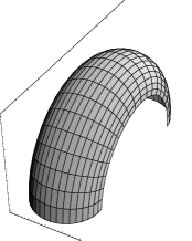
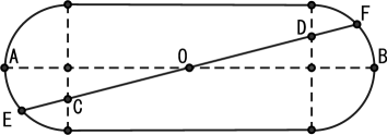
Figure 10. The image of $f$ and $\Omega$.

Let $\Pi:f([-\frac{\pi}{2},\frac{\pi}{2}]\times[-\frac{\pi}{2},\frac{\pi}{2}])\to\R^{2}$ be the projection into the $xy$-plane. Then the map $\Pi$ is injective, and the inverse map is given by

$$\Pi^{-1}:\Omega\ni{\begin{pmatrix}x\\ y\end{pmatrix}}\to{\begin{pmatrix}x\\ y\\ \left((a+\sqrt{b^{2}-y^{2}})^{2}-x^{2}\right)^{1/2}\end{pmatrix}}\in\R^{3},$$

where $\Omega$ is the closed domain in the $xy$-plane given by

$$\Omega:=\{|x|\leq a,|y|\leq b\}\cup\{(x-a)^{2}+y^{2}\leq b^{2}\}\cup\{(x+a)^{2}+y^{2}\leq b^{2}\}.$$

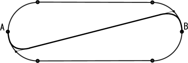
Figure 11. $\tau_{0}$ and the top view of $c_{0}$.

We take the midpoints $\mathsf{A},\mathsf{B}$ on the circular parts on the boundary of $\Omega$. Let $\mathsf{O}$ be the mid-point of $\mathsf{AB}$ which gives the center of gravity of $\Omega$. Take two points $\mathsf{C},\mathsf{D}$ on $\Omega$ as in Figure 10 (right) so that they bisect the radius of the circles of radius $b$. Let $\mathsf{E},\mathsf{F}$ be the points where $\mathsf{CD}$ meets the boundary of $\Omega$. We round the corner of the planar arc

$$\overset{\frown}{\mathsf{AE}}\cup\mathsf{EF}\cup\overset{\frown}{\mathsf{FB}},$$

and then we get a $C^{\infty}$-regular arc $\tau_{0}$ as in Figure 11 (left). The inverse image

$$\hat{\tau}_{0}:=\Pi^{-1}(\tau_{0})$$

on the torus is called the bridge arc.

Lemma 3.2.

Let $\hat{\tau}_{0}(t)$ $(0\leq t\leq 1)$ be the the bridge arc. Then it has no inflections. Moreover, it holds that

$$\operatorname{Tw}_{\hat{\tau}_{0}}(D^{\perp})-\operatorname{Tw}_{\hat{\tau}_{0}}({\mathbf{e}}_{3}^{\perp})=\pi,$$

where $D(t)$ is the Darboux vector field and ${\mathbf{e}}_{3}:=(0,0,1)$.

Proof.

Let ${\mathbf{b}}(t)$ be the unit bi-normal vector of $\hat{\tau}_{0}(t)$. Let $\theta(t)$ be the smooth function which gives the leftward angle of ${\mathbf{b}}(t)$ from ${\mathbf{e}}_{3}^{\perp}$. Like as the proof of Proposition 2.1, we can see that $D^{\perp}_{+}={\mathbf{b}}$. Then we have

$$\operatorname{Tw}_{\hat{\tau}_{0}}(D^{\perp})-\operatorname{Tw}_{\hat{\tau}_{0}}({\mathbf{e}}_{3}^{\perp})=\theta(1)-\theta(0).$$

Let ${\mathbf{t}}(t)$ be the unit tangent vector of $\tilde{\sigma}_{+}$ as a space curve. Then by definition of $\tilde{\sigma}_{+}$, we have

$${\mathbf{t}}(0)={\mathbf{t}}(1),\qquad{\mathbf{n}}(0)=-{\mathbf{n}}(1)$$

which yield

(3.2) $${\mathbf{b}}(0)={\mathbf{t}}(0)\times{\mathbf{n}}(0)=-{\mathbf{t}}(1)\times{\mathbf{n}}(1)=-{\mathbf{b}}(1).$$

Since $\hat{\tau}_{0}(t)$ is planar near $t=0,1$, ${\mathbf{b}}(t)$ is proportional to ${\mathbf{e}}_{3}^{\perp}$. Thus we have

$$\theta(1)-\theta(0)\equiv\pi\,\,\mod 2\pi\boldsymbol{Z}.$$

On the other hand, the bridge arc $\hat{\tau}_{0}(t)$ ($0\leq t\leq 1$) is symmetric with respect to the plane containing the line $\mathsf{EF}$ which is perpendicular to $xy$-plane. Moreover, the bridge arc near the the mid point $\Pi^{-1}(O)$ is planar, and the ${\mathbf{b}}(t)$ is perpendicular to the plane. Using these facts, one can easily check that $\theta(t)\geq 0$, and

$$\theta(1)-\theta(0)=\pi,$$

which proves the assertion. q.e.d.

Consider, the union of the $m$-looped $S$-arc (a planar part) and the bridge arc (a non-planar arc)

$$(\mbox{Image of }\sigma_{m})\cup\hat{\tau}_{0},$$

which gives a closed $C^{\infty}$-space curve. We denote by $c_{0}(t)=(x(t),y(t),z(t))$ ($|t|\leq\pi$) one of its parametrization. Since $\hat{\tau}_{0}$ has no inflection points, $c_{0}(t)$ is a closed embedded $C^{\infty}$-regular space curve with a generic inflection point, which corresponds to the inflection point of the original lemniscate. Figure 11(right) shows the top view of $c_{0}$.

Without loss of generality, we may assume that $t=0$ is the inflection point. Let $D(t)$ be the normalized Darboux vector field along $c_{0}(t)$. By Lemma 1.10, $F_{c_{0},D}$ gives a rectifying unknotted $C^{\infty}$-Möbius developable. Moreover, by (1.6) and Lemma 3.2 we can easily see that its Möbius twisting number $2m-1$. Since $m$ is arbitrary, its Möbius twisting number can be adjusted arbitrarily. Since the $S$-arc is planar, $c_{0}=(x(t),y(t),z(t))$ satisfies

$$\dot{z}(0)=\ddot{z}(0)=\dddot{z}(0)=z^{(4)}(0)=0.$$

On the other hand, rotating $F_{c_{0},D}$ with respect to the $z$-axis, we may assume

$$\dot{x}(0)\neq 0,\quad\dot{y}(0)=\ddot{y}(0)=0,\quad\dddot{y}(0)\neq 0,$$

that is, $c_{0}(t)$ satisfies (1)-(3) of Proposition 3.1.

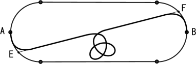
Figure 12. $\tau_{K}$ and the top view of $c_{K}$

Next, we construct a knotted rectifying $C^{\infty}$ Möbius developable. Let $K$ be an arbitrary knot diagram. Without loss of generality, we may assume that $K$ lies in the subdomain $\{|x|<a,|y|<b\}$ of $\Omega$ and moreover that $K$ lies in the lower half plane with respect to the line $EF$. Like as in Figure 12 (left), we connect $EF$ and the diagram $K$ , and denote it by $\tau_{K}$. Since $\tau_{K}$ has self-intersections, so is the inverse image $\Pi^{-1}(\tau_{K})$. By a small perturbation near the each crossing (according to its up-down status via the knot diagram $K$), we get an embedded arc $\hat{\tau}_{K}$ on the torus, which is called the $K$-bridge arc. Since the Gaussian curvature on the torus on $\Pi^{-1}(\tau_{K})$ is positive, the $K$-bridge arc $\hat{\tau}_{K}$ has no inflection points as a space curve. Let $c_{K}(t)=(x(t),y(t),z(t))$ ($|t|\leq\pi$) be the regular space curve which gives a parametrization of the union of the $m$-looped $S$-arc and the bridge arc

$$(\mbox{Image of }\sigma_{m})\cup\hat{\tau}_{K}.$$

Then by the definition of $\hat{\tau}_{K}$, $c_{K}$ is isotopic to the knot corresponding to $K$. Moreover, $c_{K}$ gives an embedded $C^{\infty}$-regular space curve with a generic inflection point. Figure 12 right is the top view of $c_{K}$. Without loss of generality we may assume that $t=0$ is the inflection point. Since the $S$-arc is planar, it satisfies

$$\dot{z}(0)=\ddot{z}(0)=\dddot{z}(0)=z^{(4)}(0)=0,$$

and we may assume

$$\dot{x}(0)\neq 0,\quad\dot{y}(0)=\ddot{y}(0)=0,\quad\dddot{y}(0)\neq 0,$$

like as in the unknotted case. Consequently, $c_{K}$ satisfies (1)-(3) of Proposition 3.1. Taking the normalized Darboux vector field of $\hat{\tau}_{K}$, we get a rectifying Möbius developable whose centerline is $\hat{\tau}_{K}$. Since $m$ is arbitrary, its Möbius twisting number can be adjusted arbitrarily. Now we have just proved Proposition 3.1.

Next we prove the following assertion:

Proposition 3.3.

Let $\gamma(t)$ $(|t|\leq\pi)$ be a centerline of rectifying $C^{\infty}$-Möbius developable $f$ satisfying the conditions $(1)$-$(3)$ in Proposition 3.1. Then there exists a family $\{\Gamma_{n}(t)\}$ $(|t|\leq\pi)$ of real analytic space curves such that

1. Each $\Gamma_{n}$ also satisfies conditions $(1)$-$(3)$ in Proposition 3.1.

2. $\{\Gamma_{n}\}_{n=1,2,\cdots}$ converges to $\gamma$ uniformly. Moreover, family of the $k$-th derivatives $(k=1,2,3,...)$ $\{\Gamma^{(k)}_{n}\}$ converges to $\gamma^{(k)}$ $C^{\infty}$-uniformly.

In particular, the rectifying developable associated with $\Gamma_{n}$ converges $f$ uniformly.

Proof.

We set

$$\gamma(t)=(x(t),y(t),z(t))\qquad(|t|\leq\pi).$$

Consider a Fourier expansion of $\gamma(t)$

$$\gamma(t)=a_{0}+\sum_{n=1}^{\infty}\biggl{(}a_{n}\cos(nt)+b_{n}\sin(nt)\biggr{)},$$

and let

$$\gamma_{n}(t)\left(=(x_{n}(t),y_{n}(t),z_{n}(t))\right):=a_{0}+\sum_{j=1}^{n}\biggl{(}a_{j}\cos(jt)+b_{j}\sin(jt)\biggr{)}\qquad(n=1,2,3,...)$$

be the $n$ th approximation of $\gamma(t)$. Then $\{\gamma_{n}\}$ is real analytic and $C^{\infty}$-uniformly converges to $\gamma$. Now we set

$$X_{n}(t):=x_{n}(t),\qquad Y_{n}(t):=y_{n}(t)-\dot{y}_{n}(0)\sin t+\ddot{y}_{n}(0)\cos t.$$

Then they are real analytic and satisfy

$$\dot{Y}_{n}(0)=\ddot{Y}_{n}(0)=0.$$

On the other hand, we have

$$\dddot{Y}_{n}(t):=\dddot{y}_{n}(t)+\dot{y}_{n}(0)\cos t+\ddot{y}_{n}(0)\sin t.$$

Since

$$\lim_{n\to 0}\dot{y}_{n}(0)=\lim_{n\to 0}\ddot{y}_{n}(0)=0,\quad\lim_{n\to 0}\dddot{y}_{n}(0)=\dddot{y}(0)\neq 0,$$

we have

$$\dddot{Y}_{n}(0)\neq 0$$

for sufficiently large $n$. Next we set

$$Z_{n}(t):= z_{n}(t)+\frac{4\ddot{z}_{n}(0)+z^{(4)}_{n}(0)}{3}\sin t-\frac{4\dot{z}_{n}(0)+\dddot{z}_{n}(0)}{3}\cos t$$

$$\qquad\quad\qquad-\frac{\ddot{z}_{n}(0)+z^{(4)}_{n}(0)}{12}\sin(2t)+\frac{\dot{z}_{n}(0)+\dddot{z}_{n}(0)}{6}\cos(2t).$$

Then it satisfies

$$\dot{Z}_{n}(0)=\ddot{Z}_{n}(0)=\dddot{Z}_{n}(0)=Z^{(4)}_{n}(0)=0.$$

If we set

$$\Gamma_{n}(t)=(X_{n}(t),Y_{n}(t),Z_{n}(t)),$$

then it satisfies (2) and (3) of Proposition 3.1. Moreover, we have

(3.3) $$\lim_{n\to 0}\dot{y}_{n}(0)=\lim_{n\to 0}\ddot{y}_{n}(0)=\lim_{n\to 0}\dot{z}_{n}(0)=\lim_{n\to 0}\ddot{z}_{n}(0)=\lim_{n\to 0}\dddot{z}_{n}(0)=\lim_{n\to 0}z^{(4)}_{n}(0)=0.$$

Since $\gamma_{n}$ converges $C^{\infty}$-uniformly to $\gamma$, so does $\Gamma_{n}$ because of (3.3).

Next we show that $\Gamma_{n}(t)$ ($t\neq 0$) has no inflection point. It can be checked by a straight-forward calculation that $\dot{\Gamma}_{n}\times\ddot{\Gamma}_{n}$ converges to $\dot{\gamma}\times\ddot{\gamma}$ on $[-\pi,\pi]$ uniformly. Thus for any $\varepsilon>0$, there exists a positive integer $N$ such that $\Gamma_{n}(t)$ ($n\geq N$) has no inflection point for $|t|\geq\varepsilon$. So it is sufficient to prove that there exists $\varepsilon>0$ such that $\dot{\Gamma}_{n}(t)\times\ddot{\Gamma}_{n}(t)$ ($|t|<\varepsilon$) vanishes only at $t=0$: The third component of the binormal vector

$$(\beta_{1},\beta_{2},\beta_{3}):=\dot{\Gamma}_{n}(t)\times\ddot{\Gamma}_{n}(t)$$

is given by

$$\beta_{3}(t)=\ddot{x}_{n}(t)(-\dot{y}(t)+\dot{y}(0)\cos t+\ddot{y}(0)\sin t)+\dot{x}(t)(\ddot{y}(t)+\dot{y}(0)\sin t-\ddot{y}(0)\cos t).$$

Since

$$\sin t =t+o(t),\qquad\cos t=1+o(t),$$

$$\dot{x}(t) =\dot{x}(0)+o(t),$$

$$\dot{y}(t) =\dot{y}(0)+t\ddot{y}(0)+o(t),$$

$$\ddot{y}(t) =\ddot{y}(0)+t\dddot{y}(0)+o(t),$$

we have

$$\beta_{3}(t)=\dot{x}_{n}(0)(\dddot{y}_{n}(0)+\dot{y}_{n}(0))t+o(t^{2}).$$

Here $o(t)$ and $o(t^{2})$ are the higher order terms than $t$ and $t^{2}$ at $t=0$, respectively. Since

$$\lim_{n\to\infty}\dot{x}_{n}(0)=\dot{x}(0)\neq 0,\quad\lim_{n\to\infty}\dot{y}_{n}(0)=0,\quad\lim_{n\to\infty}\dddot{y}_{n}(0)=\dddot{y}(0)\neq 0,$$

we can conclude that $\dot{\Gamma}_{n}(t)\times\ddot{\Gamma}_{n}(t)$ does not vanish for sufficiently small $t\neq 0$ and for sufficiently large $n$.

Finally, we show that the rectifying developable associated with $\Gamma_{n}$ converges $f$ uniformly. Then the Darboux vector field $D_{n}(t)$ of $\Gamma_{n}(t)$ has the following expression

$$D_{n}(t)=\frac{\tau_{n}(t)}{\kappa_{n}(t)}{\mathbf{t}}_{n}(t)+{\mathbf{b}}_{n}(t)$$

for $t\neq 0$, where ${\mathbf{t}}_{n}$, ${\mathbf{b}}_{n}$, $\kappa_{n}$ and $\tau_{n}$ are unit tangent vector, the unit bi-normal vector, the curvature and the torsion respectively.

Since $\Gamma_{n}(t)$ is real analytic and $t=0$ is a generic inflection point, there exists a real analytic $\R^{3}$-valued function ${\mathbf{c}}_{n}(t)$ such that ${\mathbf{c}}_{n}(0)\neq 0$ and

$$\dot{\Gamma}_{n}(t)\times\ddot{\Gamma}_{n}(t)=t{\mathbf{c}}_{n}(t).$$

Then

$${\mathbf{b}}_{n}(t)=\frac{{\mathbf{c}}_{n}(t)}{|{\mathbf{c}}_{n}(t)|}$$

gives a smooth parametrization of unit bi-normal vector of $\Gamma_{n}(t)$ near $t=0$. On the other hand, Let $M$ be the order of torsion at $t=0$. Since $\Gamma_{n}(t)$ satisfies (1)-(3) of Proposition 3.1, we have $M\geq 3$. Since $\Gamma_{n}(t)$ is real analytic, there exists a real analytic $\R^{3}$-valued function $T_{n}(t)$ such that

$$\operatorname{det}(\dot{\Gamma}_{n}(t),\ddot{\Gamma}_{n}(t),\dddot{\Gamma}_{n}(t))=t^{3}T_{n}(t).$$

Thus we have

$$\frac{\tau_{n}(t)}{\kappa_{n}(t)}=\frac{\operatorname{det}(\dot{\Gamma}_{n}(t),\ddot{\Gamma}_{n}(t),\dddot{\Gamma}_{n}(t))}{|\dot{\Gamma}_{n}(t)\times\ddot{\Gamma}_{n}(t)|^{3}}=\frac{T_{n}(t)}{|{\mathbf{c}}_{n}(t)|^{3}}.$$

Since $\Gamma_{n}(t)$ converges to $\gamma(t)$ $C^{\infty}$-uniformly, The normalized Darboux vector field $D_{n}(t)$ also converges uniformly to that of $\gamma(t)$. q.e.d.

(Proof of Theorem B.) There exists an embedded rectifying $C^{\infty}$ Möbius developable $F$ with an arbitrary isotopy type such that its centerline

$$\gamma(t)=(x(t),y(t),z(t))\qquad(|t|\leq\pi)$$

as a $2\pi$-periodic embedded space curve satisfying satisfying (1)-(3) of Proposition 3.1. By Proposition 3.3 and Corollary 1.11, there exists a sequence $\{F_{n}\}$ of rectifying $C^{\omega}$ Möbius developable uniformly converges to $F$. Then $F_{n}$ is the same isotopy type as $F$ if $n$ is sufficiently large.

(

q.e.d.)

Acknowledgements.

The authors thank Ryushi Goto for fruitful conversations on this subject. The authors also thank Wayne Rossman for a careful reading of the first draft and for valuable comments.

References

[CK]
C. Chicone and N. J. Kalton,
Flat Embeddings of Möbius strip in ,
Comm. Appl. Nonlinear Anal. 9 (2002) 31–50.
[MU]
S. Murata and M. Umehara,
Flat Surfaces with singularities in Euclidean 3-space,
preprint, math.DG/0605604.
[IT]
S. Izumiya and N. Takeuchi,
New special curve and developable surface,
Turk J. Math. 28 (2004) 153-163.
[RR1]
T. Randrup and P. Røgen,
Side of the Möbius strip,
Arch. Math., 66 (1996), 511-521.
[RR2]
T. Randrup and P. Røgen,
How to twist a knot,
Arch. Math., 68 (1997), 252-264.
[R]
P. Røgen,
Embedding and knotting of flat compact surfaces
in 3-space,
Comment. Math. Helv., 76 (2001), 589-606.
[S1] G. Schwarz, The dark side of the Möbius strip,
Amer. Math. Monthly 97 (1990) 890–897.
[S2]
G. Schwarz,
A pretender to the title ”Canonical Möbius strip”,
Pacific J. Math.,143 (1990), 195-200.
[W] W. Wunderlich, Über ein abwickelbares Möbiusband,
Monatsh. Math. 66 (1962) 276-289.