Measuring Dark Energy with Gamma-Ray Bursts and Other Cosmological Probes

Abstract

It has been widely shown that the cosmological parameters and dark energy can be constrained by using data from type-Ia supernovae (SNe Ia), the cosmic microwave background (CMB) anisotropy, the baryon acoustic oscillation (BAO) peak from Sloan Digital Sky Survey (SDSS), the X-ray gas mass fraction in clusters, and the linear growth rate of perturbations at $z=0.15$ as obtained from the 2dF Galaxy Redshift Survey. Recently, gamma-ray bursts (GRBs) have also been argued to be promising standard candles for cosmography. In this paper, we present constraints on the cosmological parameters and dark energy by combining a recent GRB sample including 69 events with the other cosmological probes. First, we find that for the $\Lambda$CDM cosmology this combination makes the constraints stringent and the best fit is close to the flat universe. Second, we fit the flat Cardassian expansion model and find that this model is consistent with the $\Lambda$CDM cosmology. Third, we present constraints on several two-parameter dark energy models and find that these models are also consistent with the $\Lambda$CDM cosmology. Finally, we reconstruct the dark energy equation-of-state parameter $w(z)$ and the deceleration parameter $q(z)$. We see that the acceleration could have started at a redshift from $z_{T}=0.40_{-0.08}^{+0.14}$ to $z_{T}=0.65_{-0.05}^{+0.10}$. This difference in the transition redshift is due to different dark energy models that we adopt. The most stringent constraint on $w(z)$ lies in the redshift range $z\sim 0.3-0.6$.

1 Introduction

The traditional cosmology has been revolutionized by modern observational techniques in distant Type Ia supernovae (SNe Ia) (Riess et al. 1998; Perlmutter et al. 1999), cosmic microwave background (CMB) fluctuations (Bennett et al. 2003; Spergel et al. 2003, 2006), and large-scale structure (LSS) (Tegmark et al. 2006). These observations suggest that the composition of the universe may consist of an extra component such as dark energy or the equations governing gravity may need a variation to explain the acceleration of the universe at the present epoch.

SNe Ia have been considered as astronomical standard candles and used to measure the geometry and dynamics of the universe. However, since it is difficult to observe SNe Ia at redshift $z\gtrsim 1.7$, this measurement has been carried out only for the $z\lesssim 1.7$ universe. Recently, it was shown that GRBs may be complementary to the SN cosmology for three reasons. First, GRBs are the most powerful explosive events at cosmological distances and in particular long-duration GRBs originate from the core collapse of massive stars. So GRBs would be detectable out to very high redshifts when the core collapse of the first stars occur (Ciardi & Loeb 2000; Lamb & Reichart 2000; Bromm & Loeb 2002, 2006). In fact, the farthest burst detected so far is GRB 050904, which is at $z=6.295$ (Kawai et al. 2006). Thus, GRBs could provide a much longer arm for measuring changes in the slope of the Hubble diagram than do SNe Ia. Second, gamma-ray photons suffer from no dust extinction when they propagate to us, so the observed gamma-ray flux is a direct measurement of the prompt emission energy. Third, there have been extensive discussions on relations between the spectral and temporal properties and some of these relations have been shown to be promising standard candles for cosmography. Schaefer (2003) derived the luminosity distances of 9 GRBs with known redshifts by using two quantities (the spectral lag and the variability) as luminosity calibrators and gave a constraint on the mass density $\Omega_{M}$. Ghirlanda et al. (2004a) found a tight relation between collimation-corrected energy $E_{\gamma}$ and the local-observer peak energy $E_{p}^{{}^{\prime}}$ (i.e., the so-called Ghirlanda relation). This relation may be physically understood as due to the viewing angle effect of an annular jet (Levinson & Eichler 2005) or Comptonization of the thermal radiation flux that is advected from the base of an outflow (Rees & & Mészáros 2005; Thompson et al. 2006). Assuming that some physical explanation (e.g., the understandings mentioned above) comes into existence, Dai, Liang & Xu (2004) used the Ghirlanda relation to constrain the cosmological parameters and dark energy. Since then, a lot of work in this so-called GRB cosmology field has been published (Ghirlanda et al. 2004b; Di Girolamo et al. 2005; Firmani et al. 2005; Friedman & Bloom 2005; Lamb et al. 2005; Liang & Zhang 2005, 2006; Xu, Dai & Liang 2005; Wang & Dai 2006a; Li et al. 2006; Su et al. 2006; Schaefer 2007; Wright 2007). Very recently, Schaefer (2007) used 69 GRBs and five relations to build the Hubble diagram out to $z=6.60$ and discussed the properties of dark energy in several dark energy models. He found that the GRB Hubble diagram is consistent with the concordance cosmology. Besides SNe Ia and GRBs, the other observations such as the shift parameter of CMB (Spergel et al. 2003, 2006), the baryon acoustic peak from Sloan Digital Sky Survey (SDSS) (Eisenstein et al. 2005), the X-ray gas mass fraction in clusters (Allen et al. 2004), the perturbation growth rate from 2dF Galaxy Redshift Survey (Hawkins et al. 2003), and the weak lensing (e.g., Schimd et al. 2007) have been used to constrain cosmological parameters and explore the properties of dark energy.

It is of growing interest that dark energy is reconstructed in a model-independent way to investigate the evolution of the deceleration parameter $q(z)$ and the dark-energy equation-of-state parameter $w(z)$ (Alam et al. 2004; Virey et al. 2005; Gong & Wang 2007; Alam et al; 2007). Evolving dark energy models had been shown to satisfy the data from SNe Ia. To reconstruct $q(z)$ and $w(z)$, Gong & Wang (2007) used the new “Gold” sample of SNe and data of SDSS and CMB, while Alam et al. (2007) adopted the new “Gold” SN sample, the SNLS sample, and data of SDSS and CMB. It is found that the result is strongly dependent on the matter density $\Omega_{M}$. The transition redshift $z_{T}\sim 0.2$ was found in reconstruction of $q(z)$ (Virey et al. 2005; Shapiro & Turner 2006; Gong & Wang 2006). Previous investigations in the construction of $w(z)$ show that the stringent constraint on $w(z)$ is in the redshift range $z\sim 0.2-0.5$ (Alam et al. 2004; Gong & Zhang 2005).

In this paper we use GRBs and the other observational data to measure the cosmological parameters and the nature of dark energy. We also reconstruct $q(z)$ and $w(z)$ out to $z>6.0$ using these observational datasets, explore the transition redshift and constrain $w(z)$. Recently, Su et al. (2006), Li et al. (2006), and Wright (2007) combined GRBs with some other cosmological probes to constrain the $\Lambda$CDM cosmology, the constant $w$ model, and the dark energy model of $w(z)=w_{0}+w_{a}(1-a)$ (where $a$ is the scale factor of the universe), respectively. In their papers, these authors adopted the distance modulus and its error (of a GRB) calculated for the concordance cosmology or the dynamical dark energy model of $w(z)=-1.31+1.48z$, which were presented by Schaefer (2007). In addition, Li et al. (2006) used the Markov Chain Monte Carlo technique to carry out global fitting. Here we use the observational data (e.g., time lag, variability, spectral peak energy $E_{\rm peak}$, minimum rise time) of GRBs to make a simultaneous fit of five correlations in any given cosmology, and consider more other cosmological probes and more dark energy models. The structure of this paper is arranged as follows: in section 2, we introduce GRBs and the other cosmological probes and describe our analytical methods. The constraints on the cosmological parameters and dark energy are presented in section 3. In section 4, we reconstruct $w(z)$ and $q(z)$. In sections 5, we summarize our findings and present a brief discussion.

2 Observational data and Analysis Methods

2.1 Type Ia Supernovae (SNe Ia)

Riess et al. (2004) reanalyzed the SN Ia dataset. They considered 14 new high-redshift events observed by the Hubble Space Telescope (HST). This led to a sample known as the “Gold” sample containing 157 SNe Ia. Recently, Riess et al. (2007) added $25$ SNe Ia to this sample. The final sample now consists of $182$ SNe Ia. The observations of SNe Ia provide the currently most direct way of probing the dark energy at low-to-medium redshifts because the used luminosity distance is directly related to the expansion history of the universe, that is,

$$d_{L}=\left\{\begin{array}[]{l}\displaystyle cH_{0}^{-1}(1+z)(-\Omega_{k})^{-1/2}\sin[(-\Omega_{k})^{1/2}I]\phantom{sssssssssssssssss}\Omega_{k}<0,\\ \displaystyle cH_{0}^{-1}(1+z)I\phantom{sssssssssssssssssssssssssssssssssssssss}\Omega_{k}=0,\\ \displaystyle cH_{0}^{-1}(1+z)\Omega_{k}^{-1/2}\sinh[\Omega_{k}^{1/2}I]\phantom{ssssssssssssssssssssssss}\,\Omega_{k}>0,\\ \end{array}\right.$$ (1)

where

$$\Omega_{k}=1-\Omega_{M}-\Omega_{DE},$$ (2)

$$I=\int_{0}^{z}dz/E(z),$$ (3)

$$E(z)=[(1+z)^{3}\Omega_{M}+f(z)\Omega_{DE}+(1+z)^{2}\Omega_{k}]^{1/2},$$ (4)

$$f(z)=\exp\left[3\int_{0}^{z}\frac{(1+w(z^{\prime}))dz^{\prime}}{(1+z^{\prime})}\right],$$ (5)

where $w(z)$ is the equation-of-state parameter for dark energy and $d_{L}$ is the luminosity distance. With $d_{L}$ in units of megaparsecs, the predicted distance modulus is

$$\mu=5\log(d_{L})+25.$$ (6)

The likelihood functions for the parameters $\Omega_{M}$ and $\Omega_{DE}$ can be determined from $\chi^{2}$ statistics,

$$\chi^{2}(H_{0},\Omega_{M},\Omega_{DE})=\sum_{i=1}^{N}\frac{[\mu_{i}(z_{i},H_{0},\Omega_{M},\Omega_{DE})-\mu_{0,i}]^{2}}{\sigma_{\mu_{0,i}}^{2}+\sigma_{\nu}^{2}},$$ (7)

where $\sigma_{\nu}$ is the dispersion in the supernova redshift (transformed to distance modulus) due to a peculiar velocity, $\mu_{0,i}$ is the observed distance modulus, and $\sigma_{\mu_{0,i}}$ is the uncertainty in the individual distance modulus. The confidence regions in the $\Omega_{M}-\Omega_{DE}$ plane can be found through marginalizing the likelihood functions over $H_{0}$ (i.e., integrating the probability density $p\propto\exp(-\chi^{2}/2)$ for all values of $H_{0}$).

2.2 Gamma-Ray Bursts (GRBs)

GRBs can be detected out to very high redshifts (Ciardi & Loeb 2000; Lamb & Reichart 2000; Bromm & Loeb 2002, 2006). They can bridge up the gap between the nearby SNe Ia and the distant CMB anisotropy. Schaefer (2007) complied 69 GRBs to make simultaneous uses of five luminosity indicators, which are relations of $\tau_{\rm lag}-L$, $V-L$, $E_{\rm peak}-L$, $E_{\rm peak}-E_{\gamma}$, and $\tau_{\rm RT}-L$. Here the time lag ($\tau_{\rm lag}$) is the time shift between the hard and soft light curves, $L$ is the luminosity of a GRB, the variability $V$ of a burst denotes whether its light curve is spiky or smooth and $V$ can be obtained by calculating the normalized variance of an observed light curve around a smoothed version of that light curve (Fenimore & Ramirez- Ruiz 2000), $E_{\rm peak}$ is the peak energy in the $\nu F_{\nu}$ spectrum, $E_{\gamma}=(1-\cos\theta_{j})E_{\rm iso}$ is the collimation-corrected energy of a GRB, and the minimum rise time ($\tau_{\rm RT}$) in the gamma-ray light curve is the shortest time over which the light curve rises by half of the peak flux of the pulse. We make a simultaneous fit to these five relations for any fixed cosmology. We perform a linear regression analysis to find a relation between observational quantities. After obtaining the distance modulus of each burst using one of these relations, we use the same method as Schaefer (2007) to calculate the real distance modulus,

$$\mu_{\rm fit}=(\sum_{i}\mu_{i}/\sigma_{\mu_{i}}^{2})/(\sum_{i}\sigma_{\mu_{i}}^{-2}),$$ (8)

where the summation runs from $1-5$ over the relations with available data, $\mu_{i}$ is the best estimated distance modulus from the $i$-th relation, and $\sigma_{\mu_{i}}$ is the corresponding uncertainty. The uncertainty of the distance modulus for each burst is

$$\sigma_{\mu_{\rm fit}}=(\sum_{i}\sigma_{\mu_{i}}^{-2})^{-1/2}.$$ (9)

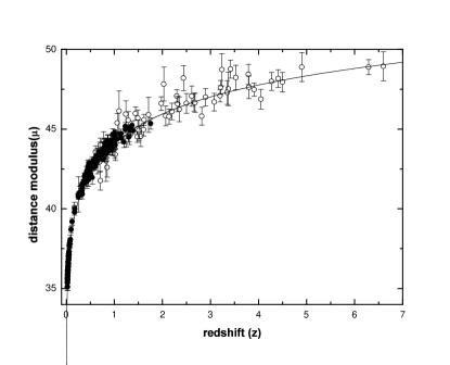
Figure 1: Hubble diagram of new 182 SNe Ia (filled circles) and 69 GRBs (open circles). The solid line is calculated for a flat cosmology: $\Omega_{M}=0.27$ and $\Omega_{\Lambda}=0.73$.

Fig.1 shows the Hubble diagram from the new “Gold” SNIa sample and 69 GRBs. The combined Hubble diagram is consistent with the concordance cosmology. GRBs can build the Hubble diagram out to $z>6.0$ (Schaefer 2007). The GRB Hubble diagram is well-behaved and describes the shape of the Hubble diagram at high redshifts. When calculating constraints on cosmological parameters and dark energy, we do not care about the slopes of the five relations because we have marginalized these parameters (Schaefer 2007). The marginalization method is to integrate over some parameter for all of its possible values. We also marginalize the nuisance parameter $H_{0}$. The $\chi^{2}$ value is

$$\chi^{2}(H_{0},\Omega_{M},\Omega_{DE})=\sum_{i=1}^{N}\frac{[\mu_{i}(z_{i},H_{0},\Omega_{M},\Omega_{DE})-\mu_{{\rm fit},i}]^{2}}{\sigma_{\mu_{{\rm fit},i}}^{2}},$$ (10)

where $\mu_{{\rm fit},i}$ and $\sigma_{\mu_{{\rm fit},i}}$ are the fitted distance modulus and its error.

2.3 Cosmic Microwave Background (CMB)

Observations of the CMB anisotropy provide us with very accurate measurements, which may be used to gain insight about dark energy and cosmological parameters (Spergel et al. 2006). We may make use of the 3-year WMAP results to get the shift parameter (Wang & Mukherjee 2006)

$$\mathcal{R}=\frac{\sqrt{\Omega_{M}}}{\sqrt{|\Omega_{k}|}}{\rm sinn}\left(\sqrt{|\Omega_{k}|}\int_{0}^{z_{\rm ls}}\frac{dz}{E(z)}\right)=1.70\pm 0.03,$$ (11)

where $E(z)\equiv H(z)/H_{0}$ and the function ${\rm sinn}(x)$ is defined as ${\rm sinn}(x)=\sin(x)$ for a closed universe, ${\rm sinn}(x)=\sinh(x)$ for an open universe and ${\rm sinn}(x)=x$ for a flat universe. To calculate the last scattering redshift $z_{\rm ls}$, we adopt $\Omega_{b}h^{2}=0.024$ and $\Omega_{M}h^{2}=0.14\pm 0.02$. To calculate $z_{\rm ls}$, we consider a fitting function:

$$z_{\rm ls}=1048[1+0.00124(\Omega_{b}h^{2})^{-0.738}][1+g_{1}(\Omega_{M}h^{2})^{g_{2}}],$$ (12)

where the quantities $g_{1}$ and $g_{2}$ are defined as $g_{1}=0.078(\Omega_{b}h^{2})^{-0.238}[1+39.5(\Omega_{b}h^{2})^{0.763}]^{-1}$ and $g_{2}=0.56[1+21.1(\Omega_{b}h^{2})^{1.81}]^{-1}$ respectively (Hu & Sugiyama 1996). The $\chi^{2}$ value is

$$\chi^{2}_{\rm CMB}=\frac{(\mathcal{R}-1.70)^{2}}{0.03^{2}}.$$ (13)

2.4 Baryon Acoustic Peak from SDSS

It is well known that the acoustic peaks in the CMB anisotropy power spectrum can be used to determine the properties of perturbations and to constrain cosmological parameters and dark energy (Spergel et al. 2003). The acoustic peaks occur because the cosmic perturbations excite sound waves in the relativistic plasma of the early universe (Peebles & Yu 1970; Holtzmann 1989). Because the universe has a fraction of baryons, the acoustic oscillations in the relativistic plasma would be imprinted onto the late-time power spectrum of the nonrelativistic matter (Peebles & Yu 1970; Eisenstein & Hu 1998). The acoustic signatures in the large-scale clustering of galaxies can also be used to constrain cosmological parameters and dark energy by detection of a peak in the correlation function of luminous red galaxies in the SDSS (Eisenstein et al. 2005). This peak can provide a “standard ruler” with which the cosmological parameters and dark energy are measured. We use the value

$$A=\frac{\sqrt{\Omega_{M}}}{z_{1}}\left[\frac{z_{1}}{E(z_{1})}\frac{1}{|\Omega_{k}|}{\rm sinn}^{2}\left(\sqrt{|\Omega_{k}|}\int_{0}^{z_{1}}\frac{dz}{E(z)}\right)\right]^{1/3},$$ (14)

measured from the SDSS data to be $A=0.469(0.95/0.98)^{-0.35}\pm 0.017$, where $z_{1}=0.35$. The $\chi^{2}$ value is

$$\chi^{2}_{\rm BAO}=\frac{(A-0.469)^{2}}{0.017^{2}}.$$ (15)

2.5 X-ray Gas Mass Fraction in Clusters

Since clusters of galaxies are the largest virialized systems in the universe, their matter content is thought to provide a sample of the matter content of the universe. A comparison of the gas mass fraction, $f_{\rm gas}=M_{\rm gas}/M_{\rm tot}$, as inferred from X-ray observations of clusters of galaxies to the cosmic baryon fraction can provide a direct constraint on the density parameter of the universe $\Omega_{M}$ (White et al. 1993). Moreover, assuming the gas mass fraction is constant in cosmic time, Sasaki (1996) showed that the $f_{\rm gas}$ measurements of clusters of galaxies at different redshifts also provide an efficient way to constrain other cosmological parameters decribing the geometry of the universe. This is based on the fact that the measured $f_{\rm gas}$ values for each cluster of galaxies depend on the assumed angular diameter distances to the sources as $f_{\rm gas}\propto(D^{A})^{3/2}$. The true, underlying cosmology should be the one which makes these measured $f_{\rm gas}$ values invariant with redshift (Sasaki 1996; Allen at al. 2004). Using the Chandra observational data, Allen et al. (2004) have got the $f_{\rm gas}$ profiles for the 26 relaxed clusters. These authors used the 26-cluster data to constrain cosmological parameters. They found $\Omega_{M}=0.245^{+0.040}_{-0.037}$ and $\Omega_{\Lambda}=0.96^{+0.19}_{-0.22}$ in the $\Lambda$CDM cosmology. This database has also been used to constrain the generalized Chaplygin gas model (Zhu 2004) and the braneworld cosmology (Zhu and Alcaniz 2005). We will combine this probe in our analysis. Following Allen et al. (2004), we calculate the $\chi^{2}$ value as

$$\chi^{2}_{\rm gas} = \left(\sum_{i=1}^{26}\frac{\left[f_{\rm gas}^{\rm SCDM}(z_{\rm i})-f_{\rm gas,\,i}\right]^{2}}{\sigma_{f_{\rm gas,\,i}}^{2}}\right)$$

$$+\left(\frac{\Omega_{\rm b}h^{2}-0.0233}{0.0008}\right)^{2}+\left(\frac{h-0.72}{0.08}\right)^{2}+\left(\frac{b-0.824}{0.089}\right)^{2},$$ (16)

where $f_{\rm gas}^{\rm SCDM}(z)=b\Omega_{b}/[(1+0.19\sqrt{h})\Omega_{M}]\times[d_{A}^{\rm SCDM}(z)/d_{A}^{\rm mod}(z)]^{1.5}$, $f_{{\rm gas},i}$ is the observational baryon gas mass fraction and $b$ is a bias factor motivated by gas-dynamical simulations which suggest that the baryon fraction in clusters is slightly lower than for the universe as a whole.

2.6 Perturbation Growth Rate from 2dF Galaxy Redshift Survey

The clustering of galaxies is determined by the initial mass fluctuations and their evolution. We can set constraints on the initial mass fluctuations and their evolution by measuring the galactic two-point correlation function. The 2dF galaxy redshift survey measured the two point correlation function at the redsift of $z=0.15$. Hawkins et al. (2003) measured the redshift distortion parameter $\beta=0.49\pm 0.09$. This result can be combined with the linear bias parameter ${\bar{b}}=1.04\pm 0.11$. So the growth factor $g$ at $z=0.15$ is $g={\bar{b}}\times\beta=0.51\pm 0.11$. Theoretically, this growth factor is cosmology-dependent. Thus, the measurement of the perturbation growth rate (PGR) $g(z=0.15)$ can be used to calculate $\chi^{2}$:

$$\chi^{2}_{\rm PGR}=\frac{(g-0.51)^{2}}{0.11^{2}},$$ (17)

which constrains the cosmological parameters and dark energy.

3 Constraints on Cosmological Parameters and Dark Energy

Using the datasets of the above observational techniques, we measure cosmological parameters and dark energy. We can combine these probes by multiplying the likelihood functions. The total $\chi^{2}$ value is

$$\chi^{2}_{\rm total}=\chi^{2}_{\rm SN}+\chi^{2}_{\rm GRB}+\chi^{2}_{\rm CMB}+\chi^{2}_{\rm BAO}+\chi^{2}_{\rm gas}+\chi^{2}_{\rm PGR}$$ (18)

3.1 The $\Lambda$CDM Cosmology

The luminosity distance in a Friedmann-Robertson-Walker (FRW) cosmology with mass density $\Omega_{M}$ and vacuum energy density (i.e., the cosmological constant) $\Omega_{\Lambda}$ is (Carroll, Press & Turner 1992)

$$d_{L} = c(1+z)H_{0}^{-1}|\Omega_{k}|^{-1/2}{\rm sinn}\{|\Omega_{k}|^{1/2}$$ (19)

$$\times\int_{0}^{z}dz[(1+z)^{2}(1+\Omega_{M}z)-z(2+z)\Omega_{\Lambda}]^{-1/2}\}.$$

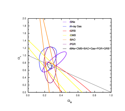
Figure 2: The $1\sigma$ joint confidence contours for $(\Omega_{M},\Omega_{\Lambda})$ from the observational datasets. The thick black line contour corresponds to all the datasets. The blue contour corresponds to 26 galaxy clusters. The red contour corresponds to 69 GRBs. The yellow contour corresponds to the CMB shift parameter. The violet contour corresponds to 182 SNe Ia. The orange contour corresponds to BAO. The purple contour corresponds to 2dF Galaxy Redshift Survey. The thin solid line represents a flat universe

We use the datasets discussed above to constrain cosmological parameters. Fig.2 shows the $1\sigma$ contours plotting in the $\Omega_{M}-\Omega_{\Lambda}$ plane. The thick black line contour from all the datasets shows $\Omega_{M}=0.27\pm 0.02$ and $\Omega_{\Lambda}=0.73\pm 0.08$ ($1\sigma$) with $\chi^{2}_{\rm min}=270.60$. The red contour shows a constraint from 69 GRBs, and for a flat universe, we measure $\Omega_{M}=0.34_{-0.10}^{+0.09}$ ($1\sigma$), which is consistent with Schaefer (2007). Because the thin solid line in Fig.2 represents a flat universe, our result from all the datasets favors a flat universe.

3.2 The Cardassian Expansion Model

The Cardassian expansion models (Freese & Lewis 2002) involve a modification of the Friedmann equation, which allows an acceleration in a flat, matter-dominated cosmology. We assume that the Cardassian expansion model is (Freese & Lewis 2002; Zhu et al. 2004)

$$H^{2}=\frac{8\pi G}{3}(\rho+C\rho^{n}).$$ (20)

This modification may arise from embedding our observable universe as a (3+1)-dimensional brane in extra dimensions or the self-interaction of dark matter. The luminosity distance in this model is

$$d_{L}=cH_{0}^{-1}(1+z)\int_{0}^{z}dz[(1+z)^{3}\Omega_{M}+(1-\Omega_{M})(1+z)^{3n}]^{-1/2}.$$ (21)

Fig.3 shows constraints on $\Omega_{M}$ and $n$. The solid contours are obtained from all the datasets. From this figure, we have $\Omega_{M}=0.28\pm 0.02$ and $n=0.02^{+0.10}_{-0.09}$ at the $1\sigma$ confidence level with $\chi^{2}_{\rm min}=272.52$. This result is consistent with the $\Lambda$CDM cosmology.

3.3 The $w(z)=w_{0}$ Model

We consider an equation of state for dark energy

$$w(z)=w_{0}.$$ (22)

In this dark energy model, the luminosity distance for a flat universe is (Riess et al. 2004)

$$d_{L}=cH_{0}^{-1}(1+z)\int_{0}^{z}dz[(1+z)^{3}\Omega_{M}+(1-\Omega_{M})(1+z)^{3(1+w_{0})}]^{-1/2}$$ (23)

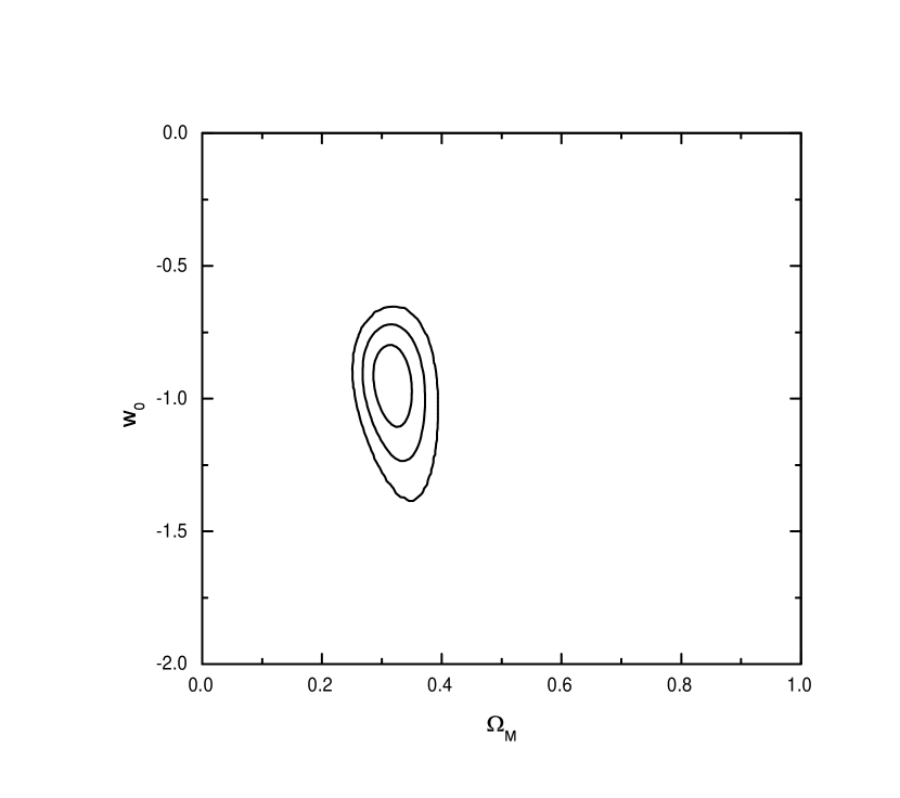
Figure 4: The $1\sigma$, $2\sigma$ and $3\sigma$ joint confidence contours for $(\Omega_{M},w_{0})$ from all the observational datasets.

Fig.4 shows the constraints on $w_{0}$ versus $\Omega_{M}$ in this dark energy model from all the datasets. From this figure, we have $\Omega_{M}=0.31\pm 0.03$ and $w_{0}=-0.95^{+0.16}_{-0.13}$ ($1\sigma)$ with $\chi^{2}_{\rm min}=272.23$.

3.4 Two-Parameter Dark Energy Models

Using the parameterization

$$w(z)=w_{0}+\frac{w_{1}z}{1+z},$$ (24)

the luminosity distance is calculated by (Chevallier & Polarski 2001; Linder 2003)

$$d_{L}=cH_{0}^{-1}(1+z)\int_{0}^{z}dz[(1+z)^{3}\Omega_{M}+(1-\Omega_{M})(1+z)^{3(1+w_{0}+w_{1})}e^{-3w_{1}z/(1+z)}]^{-1/2}.$$ (25)

Fig.5 shows the constraints on $w_{0}$ versus $w_{1}$ in this dark energy model. The solid contours are obtained from all the datasets and we find $\chi^{2}_{\rm min}=273.25$, $w_{0}=-1.08_{-0.32}^{+0.20}$ and $w_{1}=0.84_{-0.82}^{+0.40}$ ($1\sigma$) for the prior of $\Omega_{M}=0.30$. We also assume this prior in the following analysis.

Jassal, Bagla and Padmanabhan (2004) modified the above parameterization as

$$w(z)=w_{0}+\frac{w_{1}z}{(1+z)^{2}}.$$ (26)

This equation can model a dark energy component which has a similar value at lower and higher redshifts. The luminosity distance is

$$d_{L}=cH_{0}^{-1}(1+z)\int_{0}^{z}dz[(1+z)^{3}\Omega_{M}+(1-\Omega_{M})(1+z)^{3(1+w_{0})}e^{3w_{1}z^{2}/2(1+z)^{2}}]^{-1/2}.$$ (27)

Constraints on $w_{0}$ and $w_{1}$ are presented in Fig.6. From this figure, we find $\chi^{2}_{\rm min}=272.07$, $w_{0}=-1.36_{-0.48}^{+0.38}$ and $w_{1}=3.32_{-2.82}^{+2.28}$ ($1\sigma$) from all the datasets (blue contour).

The third dark energy model that we consider is (Alam et al. 2003)

$$w(z)=\frac{1+z}{3}\frac{A_{1}+2A_{2}(1+z)}{\Omega_{DE}(z)}-1,$$ (28)

where $\Omega_{DE}(z)$ is defined as

$$\Omega_{DE}(z)=A_{1}(1+z)+A_{2}(1+z)^{2}+1-\Omega_{M}-A_{1}-A_{2}.$$ (29)

Fig.7 shows the constraints on $A_{1}$ versus $A_{2}$ in this dark energy model. The solid contours are obtained from all the datasets and we find $\chi^{2}_{\rm min}=273.95$, $A_{1}=-0.43_{-1.08}^{+0.96}$ and $A_{2}=0.22_{-0.32}^{+0.29}$ ($1\sigma$).

4 Reconstruction of $w(z)$ and $q(z)$

Many dark energy models have been proposed (Copeland et al. 2006; Bludman 2006 for a recent review) and we have fitted these models using the observational data in the last section. We now explore the properties of dark energy in a model-independent way (Sahni et al. 2006 for a review). In the following we reconstruct dark energy to find new information about dark energy from most of the recent datasets. The method to reconstruct directly properties of dark energy from observations in a quasi-model independent method has been discussed (Alam et al. 2004; Gong & Wang. 2007; Alam et al. 2007). We determine the dark energy equation of state based on

$$w(z)=\frac{\frac{2}{3}(1+z)\frac{d\ln H}{dz}-1}{1-\Omega_{M}H^{-2}(1+z)^{3}}.$$ (30)

The deceleration parameter

$$q(z)=(1+z)H^{-1}\frac{dH}{dz}-1.$$ (31)

We consider the first ansatz

$$H(z)=H_{0}[(1+z)^{3}\Omega_{M}+(1-\Omega_{M})(1+z)^{3(1+w_{0}+w_{1})}e^{-3w_{1}z/(1+z)}]^{1/2}],$$ (32)

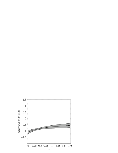
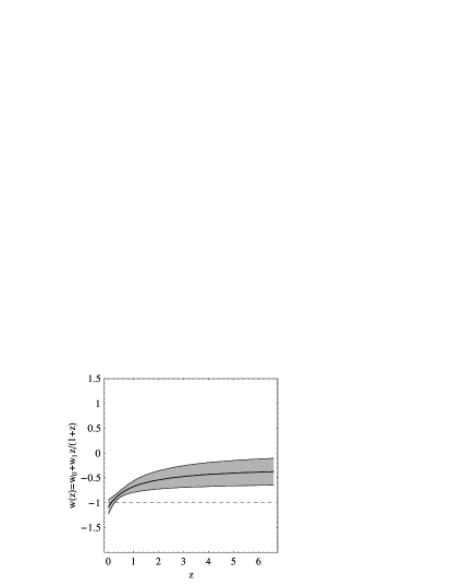
Figure 8: The evolution of $w(z)$ by fitting the model $w(z)=w_{0}+w_{1}z/(1+z)$ to all the observational data. The solid line represents the reconstructed $w(z)$. The shaded region shows the $1\sigma$ error. We can constrain the evolution of $w(z)$ up to $z>6.0$ using GRBs (bottom panel).

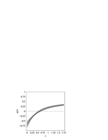
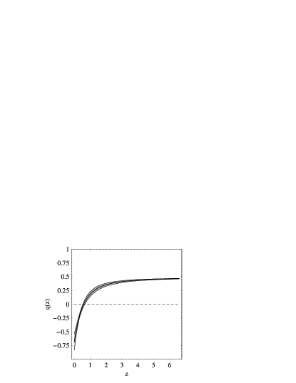
Figure 9: The evolution of $q(z)$ by fitting the model $w(z)=w_{0}+w_{1}z/(1+z)$ to all the observational data. The solid line is plotted by using the best fitting parameters. The shaded region shows the $1\sigma$ error. We can reconstruct $q(z)$ up to $z>6.0$ using GRBs (bottom panel).

which is in fact equivalent to the parameterization equation (24). The evolution of $w(z)$ is plotted in Fig.8. It is easy to see that the errors of the constraint on the equation of state become larger with redshift. The stringent constraint on $w(z)$ happens at $z=0.3\sim 0.7$. Using the GRB data, we can reconstruct $w(z)$ out to $z\sim 6.0$ in the bottom panel. The evolution of $q(z)$ is plotted in Fig.9. We can see that the transition redshift at which the expansion of the universe was from deceleration $(q(z)>0)$ to acceleration $(q(z)<0)$ is $z_{T}=0.57_{-0.07}^{+0.08}$ ($1\sigma$). This result is consistent with Riess et al. (2004) and Wang & Dai (2006a, 2006b).

We consider the second ansatz

$$H(z)=H_{0}[(1+z)^{3}\Omega_{M}+(1-\Omega_{M})(1+z)^{3(1+w_{0})}e^{3w_{1}z^{2}/2(1+z)^{2}}]^{1/2},$$ (33)

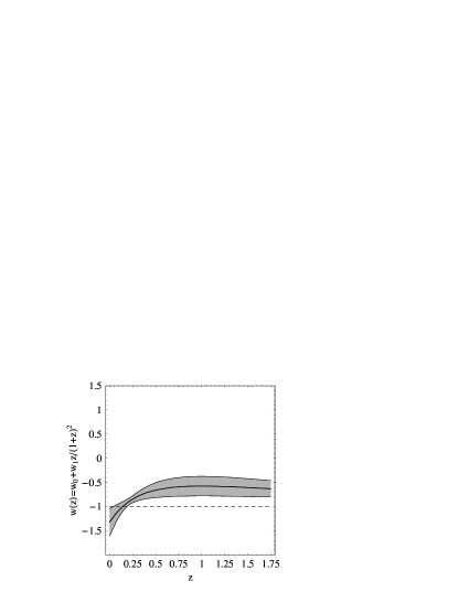
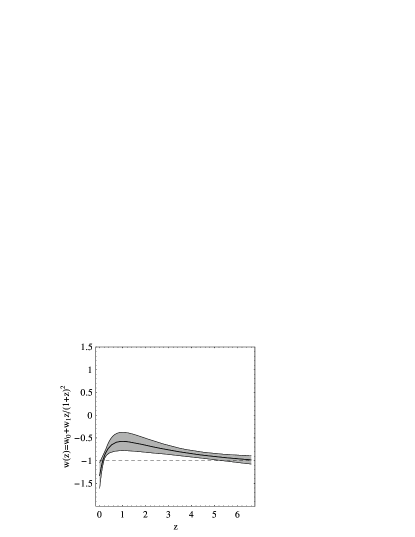
Figure 10: Same as Fig.8 but fitting the model $w(z)=w_{0}+w_{1}z/(1+z)^{2}$ to all the observational data.

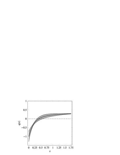
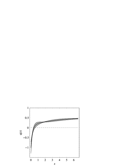
Figure 11: Same as Fig.9 but fitting the model $w(z)=w_{0}+w_{1}z/(1+z)^{2}$ to all the observational data.

which is in fact equivalent to the parameterization equation (26). The evolution of $w(z)$ is plotted in Fig.10. The stringent constraint on $w(z)$ happens at $z=0.2\sim 0.35$. Using the GRB data, we can reconstruct $w(z)$ out to $z\sim 6.0$ in the bottom panel. We find that the constraint on $w(z)$ is also stringent around $z=4.0\sim 5.0$. The evolution of $q(z)$ is plotted in Fig.11. We can see that the transition redshift is $z_{T}=0.40_{-0.08}^{+0.14}$ ($1\sigma$).

We consider the third ansatz

$$H(z)=H_{0}[(1+z)^{3}\Omega_{M}+A_{1}(1+z)+A_{2}(1+z)^{2}+1-\Omega_{M}-A_{1}-A_{2}]^{1/2},$$ (34)

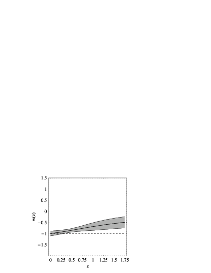
Figure 12: Same as Fig.8 but fitting the model of equation (28) to all the observational data.

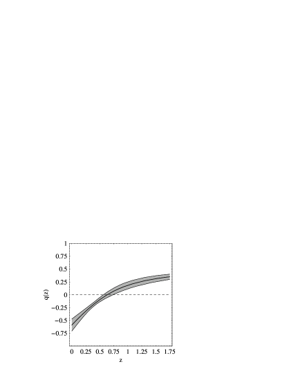
Figure 13: Same as Fig.9 but fitting the model of equation (28) to all the observational data.

which is in fact equivalent to the parameterization equation (28). The evolution of $w(z)$ is plotted in Fig.12. The stringent constraint on $w(z)$ happens at $z=0.35\sim 0.55$. Using the GRB data, we can reconstruct $w(z)$ out to $z\sim 6.0$ in the bottom panel. We find that the constraint on $w(z)$ becomes stringent around $z\sim 6.0$. The evolution of $q(z)$ is plotted in Fig.13. ¿From this figure, we can see that the transition redshift is $z_{T}=0.65_{-0.05}^{+0.10}$ ($1\sigma$).

5 Conclusions and Discussion

In this paper, we have presented the constraints on the cosmological parameters and dark energy by combining a recent GRB sample including 69 events with the 182 SNe Ia, CMB, BAO, the X-ray gas mass fraction in clusters and the linear growth rate of perturbations at $z=0.15$ as obtained from the 2dF galaxy redshift survey. We found that the mass density of the universe is $\Omega_{M}=0.27\pm 0.02$ and $\Omega_{\Lambda}=0.73\pm 0.08$ ($1\sigma$) in the $\Lambda$CDM cosmology. This result is well consistent with a flat universe. We also found that $\Omega_{M}=0.28\pm 0.02$ and $n=0.02^{+0.10}_{-0.09}$ ($1\sigma$) in the flat Cardassian expansion model. We fitted several dark energy models. Finally, we reconstructed the dark energy equation-of-state parameter $w(z)$ and the deceleration parameter $q(z)$. We found that the the cosmic acceleration could have started between the redshift $z_{T}=0.40_{-0.08}^{+0.14}$ and $z_{T}=0.65_{-0.05}^{+0.10}$ ($1\sigma$). The stringent constraints on $w(z)$ lie in the redshift range $z\sim 0.3-0.6$.

Based on our analysis, it can be seen that the preferred cosmological model is the flat $\Lambda$CDM cosmology because of a small minimum $\chi^{2}$ value, $\chi^{2}_{\rm min}=270.60$. The other models such as the Cardassian expansion model, the flat constant $w$ model, and three two-parameter dark energy models can also fit all the datasets because the minimum $\chi^{2}$ values in these models vary only from $\chi^{2}_{\rm min}=272.23$ to $\chi^{2}_{\rm min}=273.95$. Thus, we cannot reject any of these models.

It is well known that the cosmological constant suffers from the “fine tuning” problem and the coincidence problem (Zeldovich 1968; Weinberg 1989). In this paper, therefore, we have considered alternative possibilities, e.g., the Cardassian expansion model, the flat constant $w$ model, and three two-parameter dark energy models. As we have shown, all the alternative models can be reduced to the flat $\Lambda$CDM cosmology at the $1\sigma$ confidence level. So one needs more new observed data to distinguish between these models. New observations would be expected to improve the current constraints and test the flat $\Lambda$CDM model. GRBs appear to be natural events to study the universe at very high redshifts. The forthcoming GLAST will accumulate more GRB data, and in particular, its combination with Swift would lead to stronger constraints on high-redshift properties of dark energy.

Figure 3: The $1\sigma$ and $2\sigma$ joint confidence contours for $(\Omega_{M},n)$ from all the observational data.

Figure 5: The $1\sigma$ and $2\sigma$ joint confidence contours of from all the observational data in the $w(z)=w_{0}+w_{1}z/(1+z)$ model.

Figure 6: The $1\sigma$ joint confidence contours from the observational datasets in the $w(z)=w_{0}+w_{1}z/(1+z)^{2}$ model. The blue contour corresponds to all the datasets. The cyan contour corresponds to 69 GRBs. The black contour corresponds to the CMB shift parameter. The green contour corresponds to 182 SNe Ia. The dashed contour corresponds to BAO. The yellow contour corresponds to the perturbation growth rate from 2dF Galaxy Redshift Survey.

Figure 7: The $1\sigma$ and $2\sigma$ joint confidence contours for $(A_{1},A_{2})$ from all the observational data in the model of equation (28).

References

- (1) Alam, U., Sahni, V., Saini, T. D., & Starobinsky, A. A. 2003, MNRAS, 344, 1057
- (2) Alam, U., Sahni, V., Saini, T. D., & Starobinsky, A. A. 2004, MNRAS, 354, 275
- (3) Alam, U., Sahni, V., & Starobinsky, A. A. 2007, JCAP, 0702, 011
- (4) Allen, S. W., et al. 2004, MNRAS, 353, 457
- (5) Bennett, C. L., et al. 2003, ApJS, 148, 1
- (6) Bludman, S. 2006, astro-ph/0605198
- (7) Bromm, V., & Loeb, A. 2002, ApJ, 575, 111
- (8) Bromm, V., & Loeb, A. 2006, ApJ, 642, 382
- (9) Carroll, S. M., Press, W. H., & Turner, E. L. 1992, ARA&A, 30, 499
- (10) Chevallier, M., & Polarski, D. 2001, Int. J. Mod. Phys. D, 10, 213
- (11) Ciardi, B., & Loeb, A. 2000, ApJ, 540, 687
- (12) Copeland, E. J., Sami, M., & Tsujikawa, S. 2006, Int. J. Mod. Phys. D, 15, 1753
- (13) Dai, Z. G., Liang, E. W. & Xu, D. 2004, ApJ, 612, L101
- (14) Di Girolamo, T., et al. 2005, JCAP, 04, 008
- (15) Eisenstein, D. J., et al. 2005, ApJ, 633, 560
- (16) Eisenstein, D. J., & Hu, W. 1998, ApJ, 496, 605
- (17) Fenimore, E. E. & Ramirez-Ruiz, E. 2000, astro-ph/0004176
- (18) Firmani, C., Ghisellini, G., Ghirlanda, G., & Avila-Reese, V. 2005, MNRAS, 360, L1
- (19) Freese, K., & Lewis, M. 2002, Phys. Lett. B, 540, 1
- (20) Friedman, A. S. & Bloom, J. S. 2005, ApJ, 627, 1
- (21) Ghirlanda, G., Ghisellini, G., & Lazzati, D. 2004a, ApJ, 616, 331
- (22) Ghirlanda, G., et al. 2004b, ApJ, 613, L13
- (23) Gong, Y. G., & Wang, A. Z. 2007, Phys. Rev. D, 75, 043520
- (24) Gong, Y. G. & Zhang, Y. Z. 2005, Phys. Rev. D, 72, 043518
- (25) Hawkins, E. et al. 2003, MNRAS, 346, 78
- (26) Holtzmann, J. A. 1989, ApJS, 71, 1
- (27) Hu, W., & Sugiyama. 1996, ApJ, 471, 30
- (28) Jassal, H. K., Bagla, J. S., & Padmanabhan, T. 2004, MNRAS. 356, L11
- (29) Kawai, N. et al. 2006, Nature, 7081, 184
- (30) Lamb, D. Q., & Reichart, D. E. 2000, ApJ, 536, 1
- (31) Lamb, D. Q., et al. 2005, astro-ph/0507362
- (32) Levinson, A. & Eichler, D. 2005, ApJ, 629, L13
- (33) Li, H., et al. 2006, astro-ph/0612060
- (34) Liang, E. W., & Zhang, B. 2005, ApJ, 633, 611
- (35) Liang, E. W., & Zhang, B. 2006, MNRAS, 369, L37
- (36) Linder, E, V. 2003, Phys. Rev. Lett, 90, 091301
- (37) Peebles, P. J. E., & Yu, J. T. 1970, ApJ, 162, 815
- (38) Perlmutter, S., et al. 1999, ApJ, 517, 565
- (39) Rees, M. J., & Mészáros, P. 2005, ApJ, 628, 847
- (40) Riess, A. G., et al. 1998, AJ, 116, 1009
- (41) Riess, A. G., et al. 2004, ApJ, 607, 665
- (42) Riess, A. G., et al. 2007, ApJ, 659, 98
- (43) Sahni, V., & Starobinsky, A. 2006, Int. J. Mod. Phys. D, 15, 2105
- Sasaki (1996) Sasaki, S. 1996, PASJ, 48, L119
- (45) Schaefer, B. E. 2003, ApJ, 588, 387
- (46) Schaefer, B. E. 2007, ApJ, 660, 16
- (47) Schimd, C., et al. 2007, A&A, 463, 405
- (48) Shapiro, C. A., & Turner, M. S. 2006, ApJ, 649, 563
- (49) Spergel, D. N., et al. 2003, ApJS, 148, 175
- (50) Spergel, D. N., et al. 2006, astro-ph/0603449
- (51) Su, M., Fan, Z. H., & Liu, B. 2006, astro-ph/0611155
- (52) Tegmark, M., et al. 2006, Phys.Rev. D., 74, 123507
- (53) Thompson, C., Mészáros, P. & Rees, M. J. 2006, ApJ, in press (astro-ph/0608282)
- (54) Virey, J. M., et al. 2005, Phys. Rev. D., 72, 061302
- (55) Xu, D., Dai, Z. G., & Liang. E. W. 2005, ApJ, 633, 603
- (56) Wang, F. Y., & Dai, Z. G. 2006a, MNRAS, 368, 371
- (57) Wang, F. Y., & Dai, Z. G. 2006b, ChJAA, 6, 561
- (58) Wang, Y., & Mukherjee, P. 2006, ApJ, 650, 1
- (59) Weinberg, S. 1989, Rev. Mod. Phys., 61, 1
- White et al. (1993) White, S. D. M. et al. 1993, Nature, 366, 429
- (61) Wright, E. L. 2007, astro-ph/0701584
- (62) Zeldovich, Y. B. 1968, Sov. Phys, 11, 381
- (63) Zhu, Z.-H. 2004, A&A, 423, 421
- Zhu & Alcaniz (2005) Zhu, Z.-H. & Alcaniz, J. S. 2005, ApJ, 620, 7
- (65) Zhu, Z.-H., Fujimoto, M. K., & He, X. T. 2004, ApJ, 603, 365