Influence of an external magnetic field on the decoherence of a

central spin coupled to an antiferromagnetic environment

Xiao-Zhong Yuan^1,2, Hsi-Sheng Goan¹* and Ka-Di Zhu²

¹Department of Physics and Center for Theoretical Sciences, National Taiwan University, and National Center for Theoretical Sciences, Taipei 10617, Taiwan

² Department of Physics, Shanghai Jiao Tong University, Shanghai 200240, China

*e-mail: goan@phys.ntu.edu.tw

I. Introduction

Maintaining sufficient quantum coherence and quantum superposition properties is one of the most important requirements for applications in quantum information processing, such as quantum computing, quantum teleportation [1,2], quantum cryptography [3], quantum dense coding [4], and telecloning [5]. Decoherence is a process by which a quantum superposition state decays into a classical, statistical mixture of state. It arises from the unavoidable interaction and thus entanglement between quantum systems and the environments. When the environmental degrees of freedom are traced out or averaged over, the quantum states of the quantum systems are no longer pure and the quantum systems are said to have decohered.

In recent years, the decoherence behavior of a small quantum system, particularly a spin system, interacting with a large environment has attracted extensive attentions [6-17]. Different environments result in different decoherence features [18]. In some cases of the problems of a central spin coupled to an environment, a spin environment may be more appropriate to represent the actual localized background spins or magnetic defects than the delocalized oscillaor bath that is usually used. The spin environment could be lattice nuclear spins, Ising spin bath, spin-star environment or the device substrates doped with spin impurities. In Ref. [19], the decoherence behavior of a localized electron spin in the nuclear spin environment is investigated experimentally. The influence of an external magnetic field is also considered. The decoherence factor is shown to be a Gaussian type. By attributing the electron spin decoherence to quantum fluctuations of lattice nuclear spins, Ref. [20] attempts to explain the experimental results. There, the significant coupling between the electron spin and nuclear spins is assumed to be the Ising-type interaction and the coupling among nuclear spins is, however, taken to be the dipole-dipole interaction. Recently, the dynamics of the reduced density matrix for central spin systems in a spin bath described by the transverse Ising model has been analyzed using a perturbative expansion method [16] or a mean-field approximation [17,21]. The interaction between the central spin system and the spin bath for these case was assumed to be of a Ising type. It has also been reported recently that the reduced dynamics and for one- and two-spin-qubit systems in a spin-star environment [22] has been analyzed [23-26]. There, the interaction between the system and environment was assumed to be of a Heisenberg $XY$ interaction.

Antiferromagnetic materials have been reported recently to have applications in the area of quantum information processing [27-32]. It was shown that quantum computing is possible with a wide variety of clusters assemble from antiferromagnetically coupled spins [28]. An antiferromagnetic molecular ring was also suggested [32] to be a suitable candidate for the qubit implementation. The decoherence of the cluster-spin degrees of freedom in the antiferromagnetic ring is expected to arise mainly from the hyperfine coupling with the nuclear spins. Reference [30] investigated the electron spin decoherence rate of the quantum tunneling of the Néel vector in a ring type antiferromagnetic molecular magnet through the study of a nuclear spin coupled to an electron spin in the ring. In this paper, we study the opposite case. We investigate the decoherence behavior of a central spin coupled to an antiferromagnetic environment. This decoherence problem of a central spin in an antiferromagnetic environment has been investigated in Ref. [33]. A similar problem of a spin-1/2 impurity embedded in an antiferromagnetic environment has been studied in the context of quantum frustration of decoherence in Ref. [34]. There the impurity spin is coupled in real space locally to just one spin of the antiferromagnetic environment, in contrast to the central spin model where the central spin is coupled isotropically to all the spins of the environment. In Ref. [35], a large-spin impurity in a ferromagnetic bath is investigated in the context of quasi-classical partial frustration of dissipation.

In the present paper, we consider the case of how an external magnetic field will affect the decoherence behavior of a central spin in an antiferromagnetic environment. One of the interesting phenomena in antiferromagnetic materials under an applied magnetic field is the magnetic-field-induced spin-flop transition. When the applied magnetic field is increased to the critical field point, the antiferromagnetic polarization flips into the direction perpendicular to the field. This is called the spin-flop transition. The phenomena of the spin-flop transition have been observed experimentally [36, 37]. It is thus particularly interesting to investigate how the central spin coherence changes as a function of a globally applied external field in an antiferromagnetic environment, especially when the magnetic field strength is near the critical field of the flip-flop transition. Indeed, the study of the relationship between the pure-mixed state transition of a central spin and the quantum phase transition (QPT) of a bath to which the central spin is coupled has attracted much attention recently [38, 39, 40]. A QPT is driven only by quantum fluctuations (e.g., happens at zero temperature where the thermal fluctuations vanish) and can be triggered by a change of some of the coupling constants (e.g., external fields) defining the system’s Hamitonian. In Refs. [38, 39, 40] the concept of Loschmidt echo (or equivalently the decoherence factor) has been used to investigate quantum criticality in the XY and anisotropic Heisenberg spin chain models. While the quantum state fidelity approach has also been put forward in Refs. [41, 42] to study QPTs in the Dick, BCS-like and XY models. Basically, the signature of QPT (in the case of finite spin number) is the dramatic decay of the asymptotic value of the Loschmidt echo or the quantum state fidelity at the critical point. That is, the closer the bath to the QPT, the smaller the asymptotic value of the Loschmidt echo or the decoherence factor of the central spin. The extension of the investigations of quantum criticality to finite temperatures has been reported in Ref. [42]. We will show in this paper that a similar behavior of the decoherence factor of the central spin also appears in our antiferromagnetic bath model when the external magnetic field strength is tuned to near the critical field point of the flip-flop transition, a first order QPT.

It is known that the values of the critical magnetic field of the spin-flop transition can be obtained using the spin wave theory [43, 44, 45]. We thus apply, in this paper, the spin wave approximation to deal with the antiferromagnetic environment in a globally applied magnetic field at low temperatures and low energy excitations. We obtain explicitly an analytic expression of the decoherence factor for the central spin. It is found that the external magnetic field affects the decoherence process through its effect on the antiferromagnetic environment. Our results explicitly show that the decoherence factor which displays a Gaussian decay with time depends on the strength of the external magnetic field and the crystal anisotropy field in the environment. One of the important results of our present paper is that when the magnetic field is increased to the critical field point at which the spin-flop transition happens, the decoherence of the central spin reaches its highest point, consistent with the QPT witness studies in Ref. [38, 39, 40, 42]. We also investigate the influence of the environmental temperature on the decoherence of the central spin.

The paper is organized as follows. In Sec. II the model Hamiltonian is introduced and the spin wave approximation is applied to map the spin operators of the antiferromagnetic environment to bosonic operators. In Sec. III, by tracing over the environmental degrees of freedom, we calculate the time evolution of the off-diagonal density matrix elements of the central spin and obtain explicitly the decoherence time of the central spin. In Sec. IV, the influence of the environmental temperature, the environmental structure, and the external magnetic field on the decoherence behavior of the central spin are discussed. Finally a short conclusion is given in Sec. V.

II. Model and Spin Wave Approximation

We consider a single central spin coupled to an antiferromagnetic environment. It is assumed that the central spin is a spin-$\frac{1}{2}$ atom and the antiferromagnetic environment consist of atoms with spin $S$. A global magnetic field is applied to both the central spin and the antiferromagnetic environment. The total Hamiltonian can be written as

$$H = H_{S}+H_{SB}+H_{B},$$ (1)

where $H_{S}$, $H_{B}$ are the Hamiltonians of the central spin and the environment respectively, and $H_{SB}$ is the coupling term [17, 18, 33, 45]. They can be written as

$$H_{S} = -g\mu_{B}BS_{0}^{z},$$ (2)

$$H_{SB} = -\frac{J_{0}}{\sqrt{N}}S_{0}^{z}\sum_{i}(S_{a,i}^{z}+S_{b,i}^{z}),$$ (3)

$$H_{B} = J\sum_{i,\vec{\delta}}\mathbf{S}_{a,i}\cdot\mathbf{S}_{b,i+\vec{\delta}}+J\sum_{j,\vec{\delta}}\mathbf{S}_{b,j}\cdot\mathbf{S}_{a,j+\vec{\delta}}$$ (4)

$$-g\mu_{B}(B+B_{A})\sum_{i}S_{a,i}^{z}-g\mu_{B}(B-B_{A})\sum_{j}S_{b,j}^{z},$$

where $g$ is the gyromagnetic factor and $\mu_{B}$ is the Bohr magneton. For simplicity, significant interaction (Eq. 3) between the central spin and the environment is assumed to be of the Ising type with $J_{0}$ being the coupling constant [20]. $J$ is the exchange interaction and is positive for antiferromagnetic environment. The effects of the next nearest-neighbor interactions are neglected, although they may be important in some real antiferromagnets. We assume that the spin structure of the environment may be divided into two interpenetrating sublattices $a$ and $b$ with the property that all nearest neighbors of an atom on $a$ lie on $b$, and vice versa [45]. $\mathbf{S}_{a,i}$ ($\mathbf{S}_{b,j}$) represents the spin operator of the $i$th ($j$th) atom on sublattice $a$ ($b$). Each sublattice contains $N$ atoms. The indices $i$ and $j$ label the $N$ atoms, whereas the vectors $\vec{\delta}$ connect atom $i$ or $j$ with its nearest neighbors. $B$ represents a uniform external magnetic field applied in the $z$ direction. The anisotropy field $B_{A}$ is assumed to be positive, which approximates the effect of the crystal anisotropy energy, with the property of tending for positive magnetic moment $\mu_{B}$ to align the spins on sublattice $a$ in the positive $z$ direction and the spins on sublattice $b$ in the negative $z$ direction. Reference [40] has analyzed the crossover from the case of a single link of the system spin to a bath spin, to the case of the central spin model in which the system spin is uniformly coupled to all the spins of the bath. This may serve to justify the coupling Hamiltonian of Eq. (3).

We use the Holstein-Primakoff transformation,

$$S_{a,i}^{+} = \sqrt{2S-a_{i}^{+}a_{i}}a_{i},\hskip 5.69054ptS_{a,i}^{-}=a_{i}^{+}\sqrt{2S-a_{i}^{+}a_{i}},\hskip 5.69054ptS_{a,i}^{z}=S-a_{i}^{+}a_{i},$$ (5)

$$S_{b,j}^{+} = b_{j}^{+}\sqrt{2S-b_{j}^{+}b_{j}},\hskip 5.69054ptS_{b,j}^{-}=\sqrt{2S-b_{j}^{+}b_{j}}b_{j},\hskip 8.53581ptS_{b,j}^{z}=b_{j}^{+}b_{j}-S,$$ (6)

to map spin operators of the environment onto bosonic operators. We will consider the situation that the environment is in the low-temperature and low-excitation limit such that the spin operators in Eqs. (5) and (6) can be approximated as $S_{a,i}^{+}\approx\sqrt{2S}a_{i}$, and $S_{b,j}^{+}\approx b_{j}^{+}\sqrt{2S}$. This can be justified as in this limit, the number of excitation is small, and the thermal average $<a_{i}^{+}a_{i}>$ and $<b_{i}^{+}b_{i}>$ is expected to be of the order $O(1/N)$ and can be safely neglected with respected to $2S$ when $N$ is very large. The Hamiltonians $H_{SB}$ and $H_{B}$ can then be written in the spin-wave approximation as [43, 44, 45]

$$H_{SB} = -\frac{J_{0}}{\sqrt{N}}S_{0}^{z}\sum_{i}(b_{i}^{+}b_{i}-a_{i}^{+}a_{i}),$$ (7)

$$H_{B} = E_{0}+2MSJ\left(\sum_{i}a_{i}^{+}a_{i}+\sum_{j}b_{j}^{+}b_{j}\right)+2MSJ\sum_{i,\vec{\delta}}(a_{i}b_{i+\vec{\delta}}+a_{i}^{+}b_{i+\vec{\delta}}^{+})$$ (8)

$$+g\mu_{B}(B+B_{A})\sum_{i}a_{i}^{+}a_{i}-g\mu_{B}(B-B_{A})\sum_{j}b_{j}^{+}b_{j},$$

where $M$ is the number of nearest neighbors of an atom and

$$E_{0}=-2NMS^{2}J-2NSg\mu_{B}B_{A}.$$ (9)

We note here that in obtaining Hamiltonian (8) in line with the approximations of $S_{a,i}^{+}\approx\sqrt{2S}a_{i}$, and $S_{b,j}^{+}\approx b_{j}^{+}\sqrt{2S}$ in the low excitation limit, we have neglected any term containing products of four operators. The low excitations correspond to low temperatures, $T\ll T_{N}$, where $T_{N}$ is the Néel temperature [44].

Transforming Eqs. (7) and (8) to the momentum space, we have

$$H_{SB} = -\frac{J_{0}}{\sqrt{N}}S_{0}^{z}\sum_{\mathbf{k}}(b_{\mathbf{k}}^{+}b_{\mathbf{k}}-a_{\mathbf{k}}^{+}a_{\mathbf{k}}),$$ (10)

$$H_{B} = E_{0}+(2MSJ+g\mu_{B}B_{A}+g\mu_{B}B)\sum_{\mathbf{k}}a_{\mathbf{k}}^{+}a_{\mathbf{k}}$$ (11)

$$+(2MSJ+g\mu_{B}B_{A}-g\mu_{B}B)\sum_{\mathbf{k}}b_{\mathbf{k}}^{+}b_{\mathbf{k}}$$

$$+2MSJ\sum_{\mathbf{k}}\gamma_{\mathbf{k}}(a_{\mathbf{k}}^{+}b_{\mathbf{k}}^{+}+a_{\mathbf{k}}b_{\mathbf{k}}),$$

where $\gamma_{\mathbf{k}}=M^{-1}\sum_{\mathbf{\vec{\delta}}}e^{i\mathbf{k}\cdot\mathbf{\vec{\delta}}}$. Then by using the Bogoliubov transformation,

$$\alpha_{\mathbf{k}}=u_{\mathbf{k}}a_{\mathbf{k}}-v_{\mathbf{k}}b_{\mathbf{k}}^{+},$$ (12)

$$\beta_{\mathbf{k}}=u_{\mathbf{k}}b_{\mathbf{k}}-v_{\mathbf{k}}a_{\mathbf{k}}^{+},$$ (13)

where $u_{\mathbf{k}}^{2}=(1+\Delta)/2$, $v_{\mathbf{k}}^{2}=-(1-\Delta)/2$, and $\Delta=1/\sqrt{1-\gamma_{\mathbf{k}}^{2}}$, the Hamiltonians $H_{SB}$ and $H_{B}$ can be diagonalized as ($\hbar=1$)

$$H_{SB} = -\frac{J_{0}}{\sqrt{N}}S_{0}^{z}\sum_{\mathbf{k}}(\beta_{\mathbf{k}}^{+}\beta_{\mathbf{k}}-\alpha_{\mathbf{k}}^{+}\alpha_{\mathbf{k}}),$$ (14)

$$H_{B} = E_{0}^{\prime}+\sum_{\mathbf{k}}\omega_{\mathbf{k}}^{(+)}\left(\alpha_{\mathbf{k}}^{+}\alpha_{\mathbf{k}}+\frac{1}{2}\right)+\sum_{\mathbf{k}}\omega_{\mathbf{k}}^{(-)}\left(\beta_{\mathbf{k}}^{+}\beta_{\mathbf{k}}++\frac{1}{2}\right),$$ (15)

where $\alpha_{\mathbf{k}}^{+}$ ($\alpha_{\mathbf{k}}$) and $\beta_{\mathbf{k}}^{+}$ ($\beta_{\mathbf{k}}$) are the creation (annihilation) operators of the two different magnons with wavevector ${\mathbf{k}}$ and frequency $\omega_{\mathbf{k}}^{(+)}$ ($\omega_{\mathbf{k}}^{(-)}$) respectively. We note here that the coupling between different magnon modes under the spin-wave approximation is neglected. This is a consequence of neglecting terms containing products of four operators in Eq. (8) in the low temperature limit ($T\ll T_{N}$) of the spin-wave approximation, where the number of excitations of the antiferromagnetic environment is sufficiently small. For a cubic crystal system in the small $k$ approximation,

$$\omega_{\mathbf{k}}^{(\pm)} = 2MSJ\sqrt{\left(1+\frac{g\mu_{B}B_{A}}{2MSJ}\right)^{2}+2\frac{k^{2}l^{2}}{M}-1}\pm g\mu_{B}B,$$ (16)

where $l$ is the side length of cubic primitive cell of sublattice. $E_{0}^{\prime}$ is a new constant. Let $k=0$ and $\omega_{\mathbf{k}}^{(-)}=0$, a critical magnetic field,

$$B_{c}=\frac{2MSJ}{g\mu_{B}}\sqrt{\left(1+\frac{g\mu_{B}B_{A}}{2MSJ}\right)^{2}-1},$$ (17)

is obtained [43, 44, 45]. When the external magnetic field exceeds $B_{c}$, we have $\omega_{\mathbf{k}}^{(-)}<0$. This indicates that this branch of magnon is no longer stable due to the externally applied magnetic field. As a result, the antiferromagnetic polarization flips perpendicular to the field, i.e., the magnetic field induced spin-flop transition happens. The spin-flop transition demonstrates a significant change of the spin configuration in the antiferromagnetic environment. This phenomenon has been observed and investigated for many different materials [46, 47, 48]. The spin wave theory is known to describe well the low-excitation and low-temperature properties of antiferromagnetic materials. Despite this low-excitation approximation, the spin wave theory also describes well the physics for $B<B_{c}$ and the value of the critical magnetic field of the spin-flop transition in antiferromagnetic materials [43, 44, 45]. We will thus use the spin wave theory to discuss the decoherence time of the central spin under the influence of the antiferromagnetic environment when the external magnetic field is tuned to approach $B_{c}$ from below (i.e. $B\rightarrow B_{c}$ for $B<B_{c}$). It will be shown that an analytic expression for the decoherence time can be obtained.

III. Decoherence Time Calculation

In this section, we calculate the time evolution of the off-diagonal elements of the reduced density matrix for the central spin. We assume that the initial density matrix of the total systems is separable, i.e., $\rho(0)=\rho_{S}(0)\otimes\rho_{B}$. The initial state of the central spin is described by $\rho_{S}(0)$. The density matrix of the environment satisfies a thermal distribution, that is $\rho_{B}=e^{-H_{B}/T}/Z$, where $Z$ is the partition function and the Boltzmann constant has been set to one. We are interested in the dynamics of the off-diagonal elements of the reduced density matrix which are responsible for the coherence of the system. This is equivalent to calculating the time evolution of the spin-flip operator $S_{0}^{-}=|0\rangle\langle 1|$, where $|0\rangle$ and $|1\rangle$ are respectively the lower and upper eigenstates of $S_{0}^{z}$. By tracing out the environmental degrees of freedom, the time evolution of $S_{0}^{-}=|0\rangle\langle 1|$ can be written as:

$$S_{0}^{-}(t) = \textrm{tr}_{B}\left\{e^{-iHt}\left[S_{0}^{-}(0)\otimes\rho_{B}\right]e^{iHt}\right\}$$ (18)

$$= \frac{1}{Z}\textrm{tr}_{B}\left\{e^{-iHt}\left(|0\rangle\langle 1|\otimes e^{-H_{B}/T}\right)e^{iHt}\right\}$$

$$= |0\rangle\langle 1|\frac{1}{Z}\textrm{tr}_{B}\left[e^{-ig\mu_{B}t-i\frac{J_{0}}{\sqrt{N}}\sum_{\mathbf{k}}(\beta_{\mathbf{k}}^{+}\beta_{\mathbf{k}}-\alpha_{\mathbf{k}}^{+}\alpha_{\mathbf{k}})t}e^{-H_{B}/T}\right],$$

where the subscript $B$ of $\textrm{tr}_{B}$ indicates that the bath degrees of freedom are traced over. We describe briefly how Eq. (18) is obtained. Since the Hamiltonian $H_{B}$ commutes with the total Hamiltonian $H$, we may move the last term in the second line of Eq. (18) to the place next to the operator $|0\rangle\langle 1|$ and evaluate the resultant expression $e^{-iHt}|0\rangle\langle 1|e^{iHt}$ first using Eqs. (1), (2), (14) and (15). After this straightforward evaluation, the operator $|0\rangle\langle 1|$ can then be put outside of the trace $\textrm{tr}_{B}$, as shown in the last line of Eq. (18). This is because $\textrm{tr}_{B}$ does not influence the degrees of freedom of the central spin. The partition function can be evaluated as follows.

$$Z = \textrm{tr}_{B}\left(e^{-H_{B}/T}\right)$$ (19)

$$= \textrm{tr}_{B}\left[e^{-E_{0}^{\prime}-\sum_{\mathbf{k}}\omega_{\mathbf{k}}^{(+)}\left(\alpha_{\mathbf{k}}^{+}\alpha_{\mathbf{k}}+\frac{1}{2}\right)/T-\sum_{\mathbf{k}}\omega_{\mathbf{k}}^{(-)}\left(\beta_{\mathbf{k}}^{+}\beta_{\mathbf{k}}+\frac{1}{2}\right)/T}\right]$$

$$= e^{-E_{0}^{\prime}}\prod_{\mathbf{k}}e^{-\omega_{\mathbf{k}}^{(+)}/2T}\prod_{\mathbf{k}}e^{-\omega_{\mathbf{k}}^{(-)}/2T}\prod_{\mathbf{k}}\frac{1}{1-e^{-\omega_{\mathbf{k}}^{(+)}/T}}\prod_{\mathbf{k}}\frac{1}{1-e^{-\omega_{\mathbf{k}}^{(-)}/T}}.$$

Similarly, the last part of the numerator of Eq. (18) can be evaluated as

$$\textrm{tr}_{B}\left[e^{-ig\mu_{B}Bt-i\frac{J_{0}}{\sqrt{N}}\sum_{\mathbf{k}}(\beta_{\mathbf{k}}^{+}\beta_{\mathbf{k}}-\alpha_{\mathbf{k}}^{+}\alpha_{\mathbf{k}})t}e^{-H_{B}/T}\right]=e^{-ig\mu_{B}Bt}e^{-E_{0}^{\prime}}\prod_{\mathbf{k}}e^{-\omega_{\mathbf{k}}^{(+)}/2T}$$

$$\prod_{\mathbf{k}}e^{-\omega_{\mathbf{k}}^{(-)}/2T}\prod_{\mathbf{k}}\frac{1}{1-e^{i\frac{J_{0}}{\sqrt{N}}t}e^{-\omega_{\mathbf{k}}^{(+)}/T}}\prod_{\mathbf{k}}\frac{1}{1-e^{-i\frac{J_{0}}{\sqrt{N}}t}e^{-\omega_{\mathbf{k}}^{(-)}/T}}.$$ (20)

Defining decoherence factor $r(t)$ as

$$S_{0}^{-}(t)=S_{0}^{-}(0)r(t),$$ (21)

we then obtain from Eqs. (18)-(20),

$$r(t) = \frac{y^{+}y^{-}}{y_{0}^{+}y_{0}^{-}}e^{-ig\mu_{B}Bt},$$ (22)

where

$$y_{0}^{+} = \prod_{\mathbf{k}}\frac{1}{1-e^{-\omega_{\mathbf{k}}^{(+)}/T}},$$ (23)

$$y_{0}^{-} = \prod_{\mathbf{k}}\frac{1}{1-e^{-\omega_{\mathbf{k}}^{(-)}/T}},$$ (24)

$$y^{+} = \prod_{\mathbf{k}}\frac{1}{1-e^{i\frac{J_{0}}{\sqrt{N}}t}e^{-\omega_{\mathbf{k}}^{(+)}/T}},$$ (25)

$$y^{-} = \prod_{\mathbf{k}}\frac{1}{1-e^{-i\frac{J_{0}}{\sqrt{N}}t}e^{-\omega_{\mathbf{k}}^{(-)}/T}}.$$ (26)

To further evaluate the decoherence factor in the thermodynamic limit, we proceed as follows.

$$\ln y_{0}^{+} = -\sum_{\mathbf{k}}\ln\left(1-e^{-\omega_{\mathbf{k}}^{(+)}/T}\right)$$ (27)

$$= -\frac{V}{8\pi^{3}}\int\ln\left(1-e^{-\omega_{\mathbf{k}}^{(+)}/T}\right)4\pi k^{2}dk,$$

where $V$ is the volume of the environment. At low temperature such that $(\omega_{\mathbf{k}}^{(\pm)})_{max}>>T$, we may extend the upper limit of the integration to infinity. With $x=kl$ and $N=V/l^{3}$, we obtain

$$\ln y_{0}^{+} = -\frac{N}{2\pi^{2}}\int_{0}^{\infty}\ln\left(1-e^{-\omega_{\mathbf{k}}^{(+)}/T}\right)x^{2}dx.$$ (28)

In the same way, we have

$$\ln y_{0}^{-} = -\frac{N}{2\pi^{2}}\int_{0}^{\infty}\ln\left(1-e^{-\omega_{\mathbf{k}}^{(-)}/T}\right)x^{2}dx,$$ (29)

$$\ln y^{+} = -\frac{N}{2\pi^{2}}\int_{0}^{\infty}\ln\left(1-e^{i\theta}e^{-\omega_{\mathbf{k}}^{(+)}/T}\right)x^{2}dx,$$ (30)

$$\ln y^{-} = -\frac{N}{2\pi^{2}}\int_{0}^{\infty}\ln\left(1-e^{-i\theta}e^{-\omega_{\mathbf{k}}^{(-)}/T}\right)x^{2}dx,$$ (31)

where

$$\theta=\frac{J_{0}}{\sqrt{N}}t.$$ (32)

Letting

$$f^{\pm}(\theta) = \int_{0}^{\infty}\ln\left(1-e^{\pm i\theta}e^{-\omega_{\mathbf{k}}^{(\pm)}/T}\right)x^{2}dx$$ (33)

$$-\int_{0}^{\infty}\ln\left(1-e^{-\omega_{\mathbf{k}}^{(\pm)}/T}\right)x^{2}dx,$$

we can rewrite the decoherence factor as

$$r(t)=e^{-\left[\frac{f^{+}(\theta)+f^{-}(\theta)}{\theta^{2}}\right]\frac{J_{0}^{2}t^{2}}{2\pi^{2}}-ig\mu_{B}Bt}.$$ (34)

Its absolute value is then

$$|r(t)|=e^{-\textrm{Re}\left[\frac{f^{+}(\theta)+f^{-}(\theta)}{\theta^{2}}\right]\frac{J_{0}^{2}t^{2}}{2\pi^{2}}}.$$ (35)

In the thermodynamic limit, i.e., $N\rightarrow\infty$, we have, from Eq. (32), $\theta\rightarrow 0$. It is then obvious from Eq. (33) that $f^{\pm}(\theta)\rightarrow 0$ as $\theta\rightarrow 0$. To find the relation between $\theta$ and $\textrm{Re}f^{\pm}(\theta)$ in the thermodynamic limit, we calculate

$$\eta^{\pm} = \lim_{\theta\rightarrow 0}\frac{\textrm{Re}f^{\pm}(\theta)}{\theta^{2}}$$ (36)

$$= \textrm{Re}\lim_{\theta\rightarrow 0}\frac{f^{\pm}(\theta)}{\theta^{2}}$$

$$= \textrm{Re}\lim_{\theta\rightarrow 0}\frac{\int_{0}^{\infty}\frac{\mp ie^{{\pm}i\theta}e^{-\omega_{\mathbf{k}}^{(\pm)}/T}}{1-e^{{\pm}i\theta}e^{-\omega_{\mathbf{k}}^{(\pm)}/T}}x^{2}dx}{2\theta}$$

$$= \frac{1}{2}\int_{0}^{\infty}\frac{e^{-\omega_{\mathbf{k}}^{(\pm)}/T}}{(1-e^{-\omega_{\mathbf{k}}^{(\pm)}/T})^{2}}x^{2}dx.$$

From the second to the third line of Eq. (36), we have used the rule of $\lim_{x\to c}[f(x)/g(x)]=\lim_{x\to c}[f^{\prime}(x)/g^{\prime}(x)]$, where the prime denotes the derivative. The absolute value of the decoherence factor from Eq. (35) in the thermodynamic limit ($N\rightarrow\infty$, i.e., $\theta\rightarrow 0$) can then be expressed as

$$|r(t)|=e^{-\frac{J_{0}^{2}\left(\eta^{+}+\eta^{-}\right)}{2\pi^{2}}t^{2}}=e^{-\frac{t^{2}}{\tau_{0}^{2}}},$$ (37)

where the decoherence time

$$\tau_{0}=\frac{\sqrt{2}\pi}{J_{0}\sqrt{\left(\eta^{+}+\eta^{-}\right)}}.$$ (38)

Equations (37) (38) and (36) are the central result in the present paper. It indicates that the decoherence factor displays a Gaussian decay with time. The factor $t^{2}$ in the exponent is different from the Markovian approximation which usually shows a linear decay in time in the exponent. The quantities $\eta^{\pm}$ in Eq. (36) can in principle be evaluated numerically. An analytic expression can, however, be obtained [see Eq. (39)] as the external magnetic field approaches the critical field value from the below, i.e., $B\to B_{c}$ and $B<B_{c}$.

IV. Results and Discussions

We discuss the numerical results and figures calculated using Eqs. (36)-(38), and present the analytical result when $B\to B_{c}$ from below in this section. For a typical antiferromagnetic anisotropy crystal, one has $B_{A}\approx 0.1\,\mathrm{Tesla}$, $2MSJ/g\mu_{B}\approx 100\,\mathrm{Tesla}$ [43]. Our results obtained using the spin wave approximation are valid only for not too large temperatures, much smaller than the Néel temperature, $T_{N}$. According to neutron diffraction studies, the Néel temperature of antiferromagnet TbAuIn is $35\,\mathrm{K}$ [49]. Some antiferromagnets may have higher Néel temperatures. So in the following analysis, the environmental temperature is restricted below $T/g\mu_{B}=2.5\,\mathrm{Tesla}$, i.e., $T\approx 3.4\,\mathrm{K}$.

Figure 1 presents the decoherence time as a function of the external magnetic field for different temperatures with a crystal anisotropy field of $B_{A}=0.1\,\mathrm{Tesla}$. We can see that the decoherence time decreases with the increase of the external magnetic field. Figure 2 is similar to Fig. 1, except $B_{A}=0.15\,\mathrm{Tesla}$. Comparing Fig. 1 with Fig. 2, we find that the larger crystal anisotropy field suppresses the decoherence of the central spin. This field-dependent decoherence behavior may be inferred from the effective Hamiltonian, Eqs. (14)-(16). From the interaction Hamiltonian, Eq. (14), we see that the larger the difference in the magnon excitation number between the magnon $\beta_{\mathbf{k}}$ and magnon $\alpha_{\mathbf{k}}$, the stronger the effect of the environment on the central spin. When the external magnetic field is zero or absence, the two magnons, from Eq. (16), have the same frequency for a given wavevector $\mathbf{k}$. At a given temperature, the average thermal excitation number may be the same for the two magnons, but the fluctuation in the excitations for each individual magnon may not be the same at the same time. As a result, tracing over the magnon states still causes decoherence on the central spin. If the external magnetic field is increased, the magnon frequency $\omega_{\mathbf{k}}^{(-)}$ decreases but $\omega_{\mathbf{k}}^{(+)}$ increases. Consequently, the magnon mode $\beta_{\mathbf{k}}$ is easier to be excited than the magnon mode $\alpha_{\mathbf{k}}$ at a given anisotropy field and temperature. This then results in a larger magnon excitation number difference and fluctuation, and thus a stronger decoherence effect. So the decoherence time decreases with the increase of the external magnetic field. The effect of the anisotropy field on the decoherence time could be understood in a similar reasoning. At a fixed external magnetic field, both the magnon frequencies $\omega_{\mathbf{k}}^{(-)}$ and $\omega_{\mathbf{k}}^{(+)}$ increase with increasing anisotropy fields. Thus the average excitation numbers reduce, so is the fluctuation in their difference. As a consequence, the decoherence time increases with the increasing anisotropy field.

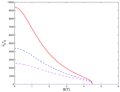
Figure 1: The decoherence time as a function of the external magnetic field for different temperatures: $T/g\mu_{B}=0.8\,\mathrm{Tesla}$ (solid curve), $T/g\mu_{B}=1.0\,\mathrm{Tesla}$ (dashed curve), and $T/g\mu_{B}=1.2\,\mathrm{Tesla}$ (dot-dashed curve). Other parameters are $M=6$, $MJ/g\mu_{B}=100\,\mathrm{Tesla}$, $B_{A}=0.10\,\mathrm{Tesla}$.

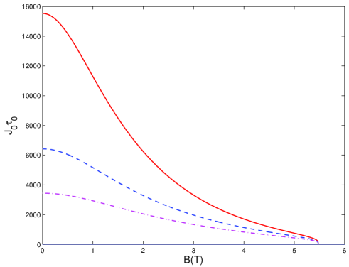
Figure 2: Same as Fig. 1, except $B_{A}=0.15\,\mathrm{Tesla}$.

An alternative way to understand the field-dependent decoherence time may be in terms of quantum correlations. There is a kind of tradeoff between the external magnetic field and the anisotropy field. The anisotropy field makes the antiferromagnets stable. On the other hand, the external magnetic field tends to reduce the antiferromagnetic order of the environment. Therefore the stronger the external magnetic field, the smaller the antiferromagnetic order. On the contrary, the larger the anisotropy field, the stronger the correlation of the antiferromagnetic environment. If the constituents (spins) of the environment maintain appreciable correlations or entanglement between themselves, then there is a restriction on the entanglement between the central spin and the environment [50, 51]. As a consequence, this sets a restriction on the amount that the central spin may decohere [16, 50, 51, 52]. Thus as far as the decoherence of the central spin is concerned, the anisotropy field has a similar effect to the exchange interaction strength between the constituents (spins) of the antiferromagnetic environment. Strong intra-environmental interaction results in a strong antiferromagnetic correlation, thus an effective decoupling of the central spin from the environment and a suppression of decoherence [50, 51]. Therefore the decoherence time increases with the increase of the anisotropy field but decreases with the increase of the strength of the external magnetic field. In summary, the results shown in Figs. 1 and 2 confirm that strong correlations within the environment suppress the decoherence effects [16, 50, 51, 52].

In Ref. [34], a similar problem of a spin-1/2 impurity coupled locally (in contrast to uniformly in the central spin model considered here) in real space to an antiferromagnetic environment has been studied in the context of quantum frustration of decoherence. There, the Hamiltonian is reduced to the case of a localized impurity spin coupled with two non-commuting spin component operators respectively to two bosonic baths. The quantum frustration is referred, in Ref. [34], to the lack of a preferred basis for the impurity spin due to the competition of the non-commutativity of the coupled spin operators to the two baths. As a result, the entanglement of the impurity spin with each one of the baths is suppressed by the other, and the decoherence phenomenon is thus frustrated. On the other hand, the effective Hamiltonian of Eqs. (2), (14) and (15) under the spin-wave approximation in our central spin model indicates clearly that the $S_{0}^{z}$ eigenstates are the preferred basis of the central spin. It also indicates that the influence of the two magnon environments seems to partially cancel each other and lead to a situation of less decoherence than a central spin coupled to a single bath. Though this may also be regarded as some kind of decoherence frustration, its cause in this spirit seems different from the quantum frustration of decoherence discussed in Ref. [34].

When the strength of the magnetic field is increased further toward the critical point where the spin-flop transition occurs, ($B=B_{c}\approx 4.5\,\mathrm{Tesla}$ for the parameters used in Fig. 1 and $B_{c}\approx 5.5\,\mathrm{Tesla}$ in Fig. 2, the decoherence time approaches zero quickly. One can obtain analytically from Eqs. (16), (36), and (38) for the decoherence time near the critical field as

$$\lim\limits_{B\rightarrow B_{c}(B<B_{c})}J_{0}\tau_{0}=\frac{4\sqrt{\pi}}{T}M^{\frac{3}{4}}J^{\frac{3}{2}}\frac{\left[g\mu_{B}(B_{c}-B)\right]^{\frac{1}{4}}}{\left(g\mu_{B}B_{c}\right)^{\frac{3}{4}}}.$$ (39)

We note that this result using spin wave theory is valid for $B<B_{c}$, i.e., before the spin-flop transition. Equation (39) indicates that when $B$ approaches $B_{c}$, the environment exerts a great influence on the central spin so that the coherence is destroyed thoroughly. This is a catastrophe for quantum computing based on such spin systems at the critical field $B_{c}$. Our result in the thermodynamic limit is consistent with those in Refs. [38, 39, 40, 42] for the case of finite spin number $N$. There, the asymptotic value of the Loschmidt echo of a bath (or equivalently the decoherence factor of a central spin) is dramatically reduced near the critical point and may serve as a good witness of QPT in the case of finite $N$. In our case, the decoherence of the central spin is enhanced near the critical point of the antiferromagnetic bath. The closer the bath to the QPT (the spin-flop transition from below, $B<B_{c}$), the smaller the decoherence time of the central spin (see Figs. 1 and 2). The decoherence reaches its maximum when the values of the external magnetic field is increased to the critical field point of the spin-flop transition. The Gaussian decay behavior of the decoherence of a central spin similar to Eq. (37) has also been reported and discussed in Refs. [38, 39, 40].

We discuss the influence of the environmental temperature on the decoherence behavior of the central spin below. The decoherence behavior is sensitive to the environmental temperature for weak external magnetic fields. High temperatures cause strong decoherence (see Fig. 1). When the external field is strong, the influence of the environmental temperature becomes minor or weak. Finally, the decoherence time is less sensitive to the change of the external magnetic field at high temperatures. This can be seen from Fig. 1 that the low temperature case (solid curve) has a sharper curve dependence than the high temperature cases (dash and dot-dash curves).

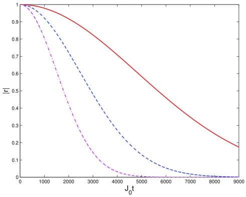
Figure 3: Time evolution of the decoherence factor for different temperatures: $T/g\mu_{B}=0.8\,\mathrm{Tesla}$ (solid curve), $T/g\mu_{B}=1.0\,\mathrm{Tesla}$ (dashed curve), and $T/g\mu_{B}=1.2\,\mathrm{Tesla}$ (dot-dashed curve). Other parameters are $M=6$, $MJ/g\mu_{B}=100\,\mathrm{Tesla}$, $B=1\,\mathrm{Tesla}$, $B_{A}=0.10\,\mathrm{Tesla}$.

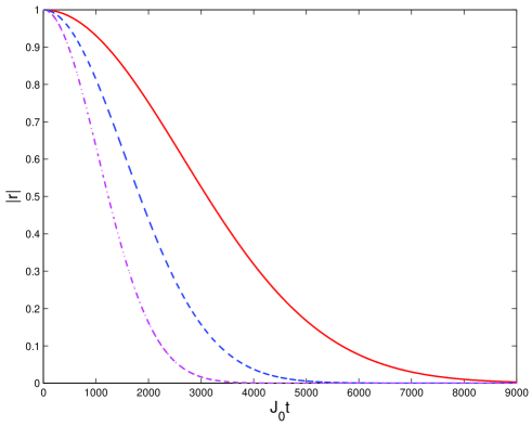
Figure 4: Same as Fig. 3, except $B=2\,\mathrm{Tesla}$.

In Fig. 3, we plot the time evolutions of the decoherence factor for different temperatures with the external magnetic field fixed at $B=1\,\mathrm{Tesla}$. As expected, the decoherence factor, under the influence of the environment, decreases with time. At a higher temperature, the decay rate is larger as shown in the figure. Figure 4 is similar to Fig. 3, except that the external magnetic field is at $B=2\,\mathrm{Tesla}$. We see again that the coherent behavior of the central spin is suppressed with the increase of the external magnetic field.

V. Conclusion

We have studied the decoherence of a central spin coupled to an antiferromagnetic environment in the presence of an external magnetic field. The results, obtained using the spin wave approximation in the thermodynamic limit, show that the decoherence factor displays a Gaussian decay with time. The decoherence time decreases, as expected, with the increase of temperatures. Furthermore, the external magnetic field promotes decoherence effects. The decoherence reaches its highest point at the critical field of the spin-flop transition, consistent with the QPT witness studies in Ref. [38, 39, 40, 42]. In contrast, the strong anisotropy field suppress decoherence of the antiferromagnetic environment on the central spin. Therefore, in order to reduce the loss of coherence of the the central spin, we could decrease the environmental temperature, eliminate the external magnetic field, and choose the antiferromagnetic surrounding or underlying antiferromagnetic materials with a strong crystal anisotropy field.

VI. Acknowledgments

X.Z.Y. and H.S.G. would like to acknowledge support from the National Science Council, Taiwan, under Grants No. NSC95-2112-M-002-018 and No. NSC95-2112-M-002-054, and support from the focus group program of the National Center for Theoretical Sciences, Taiwan. H.S.G. also acknowledges support from the National Taiwan University under Grant No. 95R0034-02 and is grateful to the National Center for High-performance Computing, Taiwan, for computer time and facilities. X.Z.Y. also acknowledges support from the National Natural Science Foundation of China under Grant No. 10647137.

References

- [1] C. H. Bennett, G. Brassard, C. Crépeau, R. Jozsa, A. Peres, W.K. Wootters, Phys. Rev. Lett. 70, 1895 (1993).
- [2] D. Bouwmeester, J.W. Pan, K. Mattle, M. Eibl, H. Weinfurter, A. Zeilinger, Nature (London) 390, 575 (1997).
- [3] C. H. Bennett, G. Brassard, A.K. Ekert, Sci. Am. (Int. Ed.) 267, 50 (1992).
- [4] C. H. Bennett, S.J. Wiesner, Phys. Rev. Lett. 69, 2881 (1992).
- [5] M. Murao, D. Jonathan, M.B. Plenio, V. Vedral, Phys. Rev. A 59, 156 (1999).
- [6] A. J. Leggett, S. Chakravarty, A. T. Dorsey, M. P.A. Fisher, A. Garg, W. Zwerger, Rev. Mod. Phys. 59, 1 (1987).
- [7] U. Weiss, Quantum dissipative systems (World Scientific, Singapore, 1999), 2nd ed.
- [8] W. H. Zurek, Rev. Mod. Phys. 75, 715 (2003).
- [9] A. Melikidze, V.V. Dobrovitski, H.A. De Raedt, M.I. Katsnelson, B. N. Harmon, Phys. Rev. B 70, 014435 (2004).
- [10] N. V. Prokof’er, P.C.E. Stamp, Rep. Prog. Phys. 63, 669 (2000).
- [11] A. Garg, Phys. Rev. Lett, 70, 1541 (1993); Phys. Rev. Lett. 74, 1458 (1995).
- [12] J. Schliemann, A. V. Khaetskii, D. Loss, Phys. Rev. B 66, 245303 (2002).
- [13] I. A. Merkulov, Al.L. Efros, M. Rosen, Phys. Rev. B 65, 205309 (2002).
- [14] A. V. Khaetskii, D. Loss, L. Glazman, Phys. Rev. Lett. 88, 186802 (2002).
- [15] J. Shao, P. Hänggi, Phys. Rev. Lett, 81, 5710 (1998).
- [16] S. Paganelli, F. de Pasquale, S.M. Giampaolo, Phys. Rev. A 66, 052317 (2002).
- [17] M. Lucamarini, S. Paganelli, S. Mancini, Phys. Rev. A 69, 062308 (2004).
- [18] S. Brouard, J. Plata, Phys. Rev. A 70, 013413 (2004).
- [19] E. Abe, K. M. Itoh, J. Isoya, S. Yamasaki, Phys. Rev. B 70, 033204 (2004).
- [20] W. M. Witzel, R. D. Sousa, S. Das Sarma, Phys. Rev. B 72, 161306 (R) (2005).
- [21] X. San Ma, A. Min Wang, X. Dong Yang, and H. You, J. Phys. A 38, 2761 (2005).
- [22] A. Hutton and S. Bose, Phys. Rev. A 69, 042312 (2004).
- [23] H. P. Breuer, Phys. Rev. A 69, 022115 (2004).
- [24] H. P. Breuer, D. Burgarth, and F. Petruccione, Phys. Rev. B 70, 045323 (2004).
- [25] Y. Hamdouni, M. Fannes, and F. Petruccione, Phys. Rev. B 73, 245323 (2006).
- [26] X. Z. Yuan, H.-S. Goan, K. D. Zhu, Phys. Rev. B 75, (2007).
- [27] M. C. Arnesen, S. Bose, V. Vedral, Phys. Rev. Lett. 87, 017901 (2001).
- [28] F. Meier, J. Levy, D. Loss, Phys. Rev. B 68, 134417 (2003).
- [29] B. Q. Jin, V.E. Korepin, Phys. Rev. A 69, 062314 (2004).
- [30] F. Meier, D. Loss, Phys. Rev. Lett. 86, 5373 (2001).
- [31] A. Chiolero, D. Loss, Phys. Rev. Lett. 80, 169 (1998).
- [32] F. Troiani, A. Ghirri, M. Affronte, S. Carretta, P. Santini, G. Amoretti, S. Piligkos, G. Timco, and R. E. P. Winpenny, Phys. Rev. Lett. 94, 207208 (2005)
- [33] X. Z. Yuan, K. D. Zhu, Europhys. Lett. 69, 868 (2005).
- [34] E. Novais, A. H. Castro Neto, L. Borda, I. Affleck, G. Zarand, Phys. Rev. B 72, 014417 (2005).
- [35] H. Kohler, F. Sols, New J. of phys. 8, 149 (2006).
- [36] G. P. Felcher, R. Kleb, V. Jaccarino, J. Appl. Phys. 50, 1837 (1979).
- [37] U. Welp, A. Berger, D. J. Miller, V. K. Vlasko-Vlasov, K. E. Gray, J. F. Mitchell, Phys. Rev. Lett. 83, 4180 (1999).
- [38] H. T. Quan, Z. Song, X. F. Liu, P. Zanardi, C. P. Sun, Phys. Rev. Lett. 96, 140604 (2006).
- [39] F. M. Cucchietti, S. F. Vidal, J. P. Paz, Phys. Rev. A 75, 032337 (2007).
- [40] D. Rossini, T. Calarco, V. Giovannetti, S. Montangero, R. Fazio,, Phys. Rev. A 75, 032333 (2007).
- [41] P. Zanardi, N. Paunković, Phys. Rev. E 74, 031123 (2006).
- [42] P. Zanardi, H. T. Quan, X. G. Wang, C. P. Sun, Phys. Rev. A 75, 032109 (2007).
- [43] O. Madelung, Introduction to Solid-State Theory, (Springer series in solid-state sciences, V. 2).
- [44] K. Yosida, Theory of Magnetism, (Springer series in solid-state sciences, V. 122).
- [45] C. Kittel, Quantum Theory of Solids, (John Wiley and Sons, Inc., New York, 1963).
- [46] S. Yunoki, Phys. Rev. B 65, 092402 (2002).
- [47] Ana L. Dantas, Selma R. Vieira, N. S. Almeida, A. S. Carriço, Phys. Rev. B 71, 014409 (2005).
- [48] Joonghoe Dho, C. W. Leung, Z. H. Barber, M. G. Blamire, Phys. Rev. B 71, 180402 (2005).
- [49] Ł. Gondek, A. Szytuła, M. Bałanda, W. Warkocki, A. Szewczyk, M. Gutowska, Solid State Commun. 136, 26 (2005).
- [50] C. M. Dawson, A. P. Hines, R. H. McKenzie, G. J. Milburn, Phys. Rev. A 71, 052321 (2005).
- [51] L. Tessieri, J. Wilkie, J. Phys. A 36, 12305 (2003).
- [52] H. Hwang, P. J. Rossky, J. Chem. Phys. 120, 11380 (2004).