Simulation of time evolution with the MERA

Abstract

We describe an algorithm to simulate time evolution using the Multi-scale Entanglement Renormalization Ansatz (MERA) and test it by studying a critical Ising chain with periodic boundary conditions and with up to $L\approx 10^{6}$ quantum spins. The cost of a simulation, which scales as $L\log(L)$, is reduced to $\log(L)$ when the system is invariant under translations. By simulating an evolution in imaginary time, we compute the ground state of the system. The errors in the ground state energy display no evident dependence on the system size. The algorithm can be extended to lattice systems in higher spatial dimensions.

The role of numerical simulations in many branches of physics is becoming more and more fundamental as the complexity of the systems of interest increases dmrgrev . Recently, the injection of quantum information concepts has opened up the possibility of significant improvements in our ability to simulate strongly correlated quantum many-body systems. The entanglement present in the many-body wave function has been identified as a major limiting factor in numerical simulations. Accordingly, a big effort has been made within the quantum information community to devise new simulation strategies that, building upon the matrix product state (MPS) MPS and the density matrix renormalization group DMRG , include a careful description of entanglement (see e.g. Refs. TEBD ; vMPS ; PEPS ; ER ; MERA ; eisert ; briegel ). In particular, the notion of entanglement renormalization —the systematic removal of short-ranged entanglement in the system— has been put forward as a means to obtain an efficient real-space renormalization group (RG) transformation for quantum systems on a lattice ER . Relatedly, the Multi-scale Entanglement Renormalization Ansatz (MERA) has been proposed as a variational many-body wave function to describe ground states MERA . It has been already demonstrated that the MERA offers a particularly accurate and compact representation of critical and non-critical ground states in 1D lattices ER . However, the existence of an efficient algorithm to systematically compute the MERA for ground states is not yet demonstrated.

In this paper we present an algorithm, referred to as the t-MERA algorithm, to simulate time-evolution with the MERA. For simplicity, we describe and test the approach in a one-dimensional system, namely a critical Ising chain with periodic boundary conditions. However, the algorithm can be readily generalized to lattice systems in higher dimensions. The cost of simulating $L$ spins in an inhomogeneous system scales as $L\log(L)$. We exploit translational invariance to further reduce this cost to $\log(L)$, allowing us to accurately address systems of up to $2^{20}\approx 10^{6}$ spins with very modest computational resources.

The t-MERA algorithm is inspired in the time-evolving block decimation (TEBD) algorithm for MPS TEBD . As in the latter, the tensors in the ansatz are updated so as to account for the action of a two-body gate acting between two neighboring lattice sites. However, while in an MPS the update involves only the tensor immediately close to those sites and is performed with a simple singular value decomposition TEBD , in the case of a MERA the update is given by a more sophisticated optimization, defined by a fidelity maximization, as described below.

Figure 1: (Color online) a) MERA tensor structure with periodic boundary conditions and $\ell=3$. b) Schematic representation of the fidelity (3). Black (red) tensors represents the tensors inside the causal cone of $|\psi\rangle$ ($|\tilde{\psi}\rangle$). Blue tensors (at sides) are outside the causal cone, thus they are contracted for free (c)). d-e) Schematic representation of the expressions (4) and (5).

We consider a many body quantum system composed of $L=2^{\ell+1}$ sites, each of them described by a local Hamiltonian and some nearest neighbor interactions $\mathcal{H}_{i,i+1}:\mathbb{C}^{d^{2}}\rightarrow\mathbb{C}^{d^{2}}$ nnn . The global Hamiltonian is then

$$\mathcal{H}=\sum_{\langle k\rangle}\mathcal{H}_{k,k+1},$$ (1)

where $k=1,L$ with $L+1\equiv 1$ for periodic boundary conditions. Consider the ensemble of wave functions that can be described exactly via a given MERA structure

$$\mathcal{M}:=\Big{\{}|\psi\rangle\in\mathcal{H}_{d}^{\otimes L}\Big{|}|\psi\rangle=$$ (2)

$$=\prod_{i=1}^{\ell}\prod_{j=1}^{2^{i}}\lambda_{\beta_{1}^{\prime},1}^{\beta_{2}^{\prime},1}\hat{\chi}[j,i]\hat{\Gamma}[j,i]\delta_{\alpha^{\prime}_{2j,i}}^{\beta_{2j,i}}\delta_{\alpha^{\prime}_{2j+1,i}}^{\beta_{2j+1,i}}\delta_{\alpha_{j,i-1}}^{\beta^{\prime}_{j,i}},\Big{\}}$$

with $\hat{\chi}[j,i]=\chi[i]_{\alpha_{2j},\alpha_{2j+1}}^{\alpha_{2j}^{\prime},\alpha_{2j+1}^{\prime}}$ unitary operator $(\hat{\chi}\hat{\chi}^{\dagger}=\hat{\chi}^{\dagger}\hat{\chi}=1)$, $\hat{\Gamma}[j,i]=\Gamma[i]_{\beta_{2j-1},\beta_{2j}}^{\beta_{j}^{\prime}}$ isometry $(\hat{\Gamma}^{\dagger}\hat{\Gamma}=1)$, $\sum|\lambda|^{2}=1$ and $\alpha,\beta,\alpha^{\prime},=1,\dots,\textrm{min}(m,d^{\ell-i+1})$, where $i$ counts the tensor network level and $j$ the position on a given level ER ; note1 . The MERA structure is represented in Figure 1 a. As shown in ER the tensors $\hat{\chi}$ can be interpreted as disentanglers. The parameter $m$ is the dimension of the projected space and is related with the number of state kept $m_{\mathrm{e}ff}$ in the reduced density matrix of half system in the Density Matrix Renormalization Group algorithm DMRG . Indeed, a simple calculation can show that the two quantities are related through $m_{\mathrm{e}ff}=m^{2(log_{2}L-1)}$. Notice that the logarithmic scaling allows to describe the quantum correlations present in 1D critical chains logscaling ; entrev .

The simulation of time evolution is achieved by updating the MERA when the operator $U=e^{-iHt}$ is applied to the state. When the time is real, $t\in R$, U is an unitary evolution, whereas when $t$ is imaginary, $t=-i\eta$ with $\eta\in R$, $U=e^{-H\eta}$ is an euclidean time operator that in the large $t$ limit projects onto the ground state of $H$. We use the Suzuki-Trotter decomposition at a given order to obtain a sequence of two sites operators $U_{k,k+1}$ to be applied to the initial ansatz $|\psi_{0}\rangle$ trotter . The problem is then reduced to the application of the operators $U_{k,k+1}$ to the MERA and to absorb it, recovering the original structure with the minimum error. In other words, given a $|\psi\rangle\in\mathcal{M}$ and $U_{k,k+1}$ we want to find $|\tilde{\psi}\rangle\in\mathcal{M}$ such that

$$\mathcal{\bar{F}}=\textrm{max}_{\begin{subarray}{c}|\tilde{\psi}\rangle\in\mathcal{M}\end{subarray}}^{~{}~{}~{}}|\mathcal{F}|=\textrm{max}_{\begin{subarray}{c}|\tilde{\psi}\rangle\in\mathcal{M}\end{subarray}}^{~{}~{}~{}}\big{|}\langle\tilde{\psi}|U_{k,k+1}|\psi\rangle\big{|}.$$ (3)

To perform such maximization efficiently, we implement a recursive procedure andan optimization of every element belonging to the causal cone causalcone . The maximization is carried out for each tensor separately as no exact method is known (notice that in the TEBD algorithm this is performed exactly via a single SVD TEBD ). We first set $|\tilde{\psi}\rangle=|\psi\rangle$ and we compute the trace fidelity $\mathcal{F}=Tr(U_{k,k+1}\rho^{\chi,\ell})$ with $\rho^{\chi,\ell}=|\psi\rangle\langle\psi|$ as represented in Figure 1 b. As shown in TTN the trace fidelity is equal to the contraction of the part of the tensor network inside the causal cone, i.e. the part of the network that can be influenced by a local operation which, at each level, is composed of maximum two unitaries $\chi$ or three isometries $\Gamma$ (see Fig. 1 c). Indeed, as shown in the figure, due to the properties of the tensor involved, the part of the network outside the causal cone is contracted for free. Thus, to compute $\mathcal{F}$ only the reduced density matrix $\rho_{CC}^{\chi,\ell}$ of the two involved sites is needed and the application of any local operator $U_{k,k+1}$ will result in a modification of the tensors inside its causal cone. Notice that the fidelity can be expressed as a function of the reduced density matrix at the upper level writing explicitly its dependence with the tensors at the last level, that is

$$\mathcal{F}=Tr(U_{k,k+1}\chi[k,\ell]\chi[k+1,\ell]\rho_{CC}^{\Gamma,\ell}\tilde{\chi}[k,\ell]^{\dagger}\tilde{\chi}[k+1,\ell]^{\dagger}),$$ (4)

as shown in Figure 1 d. We first update a single tensor, e.g. $\tilde{\chi}[k,\ell]^{\dagger}$, contracting all the other tensors obtaining

$$\mathcal{F}=Tr(\tilde{\chi}[k,\ell]^{\dagger}\mathcal{B}),$$ (5)

as shown in Fig. 1 e noteB . The maximum of the fidelity is given by $\tilde{\chi}[k,\ell]=V$ where $V$ is the unitary part of the polar decomposition of the matrix $\mathcal{B}=VP$ thpolar . We then write the analogous relation (5) related to the second tensor to be maximized and update $\tilde{\chi}[k+1,\ell]$. The maximization can be repeated until convergence is reached. We can now express explicitly the relation (4) with its dependence from the isometries of the last level $\Gamma$s and the updated $\tilde{\chi}$s

$$\mathcal{F}=Tr(\tilde{U}_{k,k+1}\Gamma[k,\ell]\Gamma[k+1,\ell]\Gamma{[k+2,\ell]}$$ (6)

$$\rho_{CC}^{\chi,\ell-1}\tilde{\Gamma}[k,\ell]^{\dagger}\tilde{\Gamma}[k+1,\ell]^{\dagger}\tilde{\Gamma}[k+2,\ell]^{\dagger}).$$

with $\tilde{U}_{k,k+1}=\tilde{\chi}[k,\ell]^{\dagger}\tilde{\chi}[k+1,\ell]^{\dagger}U_{k,k+1}\chi[k,\ell]\chi[k+1,\ell]$. To perform the fidelity maximization we repeat the previous operations optimizing the $\Gamma$s separately, defining at every optimization a new operator $\mathcal{B}$ and performing its polar decomposition. Notice that in this case $\mathcal{B}$ is a rectangular matrix and $V$ is an isometry. Finally the same procedure is repeated for every level of the tensor structure, until the top is reached. Particular attention is needed to perform the update of the uppermost $\Gamma$s and the vector $\lambda$. In this case one can again write the problem to be optimized in the same way as before. However both $\Gamma$s can be updated together: once computed the operator $\mathcal{B}$ it can be Schmidt decomposed in two different tensors each one defining the new $\Gamma[j,1]$s. The singular values obtained define the new vector $\lambda$. In the case of euclidean evolution, a renormalization (enforcing $\sum_{i}|\lambda_{i}|^{2}=1$) will take in account of the loss of norm of $|\psi^{\prime}\rangle$ due to the non unitarity of the euclidean operator $\hat{U}$.

Figure 2: (Color online) Convergence of the computed ground state energy $E(L)$ for $L=2^{\ell},\ell=8,10\dots 20$ to the exact ground state energy $E_{ex}(L)$ with periodic boundary conditions lieb .

We have build an approximation of the wave function $U_{k,k+1}|\psi\rangle$ which maximizes the fidelity $\mathcal{F}$ and $|\tilde{\psi}\rangle\in\mathcal{M}$. We then repeat the operations previously described for every operator $U_{k,k+1}$ and for every Trotter step $\Delta t$ until the desired convergence is reached.

In conclusion, we sketch the algorithm scheme for the sake of clarity:

1. Decompose the evolution operator in operators that act on nearest neighbor physical sites $U_{k,k+1}$ with the Trotter decomposition at desired order.

2. For every $U_{k,k+1}$ and for every Trotter step, set $|\psi\rangle\rightarrow|\tilde{\psi}\rangle$ and perform the following actions:

   1. For every level $i>1$

   2. Find the optimal $\chi$s obtained by maximization of the fidelity (4). Replace the old $\chi$s with the new ones, $\tilde{\chi}$s, obtained as unitary part of the polar decomposition of the operator $\mathcal{B}$. If necessary repeat the maximization until convergence is reached.

   3. Repeat step (a) to update the $\Gamma$s maximizing the fidelity (6). Again repeat the process if needed.
      when the uppermost level is reached ($i=1$)

   4. Find the new isometries and the new norm vector via a Schmidt decomposition of unitary part of the operator $\mathcal{B}$. If euclidean evolution is simulated, renormalize the vector of the singular values to obtain $\tilde{\lambda}$. Set $|\tilde{\psi}\rangle\rightarrow|\psi\rangle$.

3. When desired, perform one and two sites observables measurement computing $Tr(\hat{O}_{k,k^{\prime}}\rho_{CC}^{\chi,\ell})$ as described in TTN .

The t-MERA algorithm, as described before, requires an impressive limited amount of resources (e.g. few hours on a laptop for $L=2^{14}$ for the translational invariant case), polynomial both in memory and time as a function of the system size and of the desired $m$: given $L$ and $m$ the memory resources scale as $\mathcal{O}(m^{4}L\log L)$ that is the memory needed to store the tensor structures ER . The computational times are dominated by the tensor contractions needed to compute the operator $\mathcal{B}$ during the trace fidelity maximization, made of at most $m^{9}$ operations TTN . As for every Trotter step one needs to compute $\mathcal{O}(L\log L)$ different $\mathcal{B}$ operators (one for each link and level), the algorithms scales as $\mathcal{O}(m^{9}L\log L)$. Even though the scaling with the projected size $m$ is polynomial, it might still need a huge amount of computational time for big $m$ due to the high polynomial scaling power which might result in a limitation of this algorithm usefulness. However, as we show later on, already with $m=4$ we obtained very high precisions. More important and differently from previous proposed algorithms, the projected space size $m$ needed to keep the error constant does not depend on the system size $L$, allowing to increase the size of the system up to thousands sites with only a linear-log cost in term of computational resources. Finally, if the Hamiltonian is traslational invariant, one can take advantage of this symmetry reducing the simulation cost to $O(\log L)$ allowing impressive system size to be studied as shown in the following.

Figure 3: (color online) Energy $E(L)$ as a function of the system size ($L=2^{\ell},\ell=8,\dots,20$) for the critical Ising model (blue circles), $m=4$, $dt=0.1$ and $T_{f}=800$. Red full line represents the exact thermodinamical limit $E_{\infty}^{ex}=-4/\pi$. Inset: Difference of the computed energy with respect to thermodinamical limit $\Delta E=E(L)-E_{\infty}^{ex}$. The red line represents the exact scaling.

Results: We now apply the t-MERA algorithm to the study of the Ising chain ground state as a benchmark of the precision of the results that can be obtained. The Ising model is defined as

$$\mathcal{H}=-\sum_{<k>}h\,\sigma_{k}^{z}+\sigma_{k}^{x}\sigma_{k+1}^{x},$$ (7)

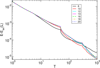
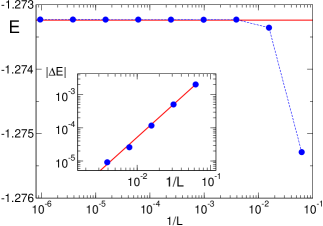
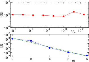
where $<k>$ describes periodic boundary conditions. The model is known to be critical for $h=1$ and it can be solved exactly via the usual mapping to the fermionic operators lieb . In Fig. 2 we plot some typical convergence of the ground state energy as a function of the imaginary time $T$ for the critical ($h=1$) Ising model with periodic boundary conditions starting from the completely polarized state $|\psi_{0}\rangle=|\uparrow\dots\uparrow\rangle$. We start with disentanglers set to the identity and after some time $T_{i}$ we switch on the optimization procedure for the $\chi$s as can be seen in Fig. 2 where a non smooth behavior is present. In Figure 3 we plot the finite size scaling energy resulting from our simulations at given final time $T_{f}$: the resulting energy is $E(\infty)=1.273229\dots$ with an error with respect to the exact solution of $\Delta E=10^{-5}$. As clearly seen in the inset of Fig. 3 with this algorithm we can accurately reproduce the finite size scaling of properties such as the energy. Finally in Fig.4 A we show the error $\delta E=E(L)-E_{ex}(L)$ at given time $T_{f}$ of the computed energy $E(L)$ with respect to the exact energy for finite size $E_{ex}(L)$ as a function of the system size $L$: the error appears to be size independent. This is the most noticeable feature of the t-MERA algorithm and it reflects the underlaying MERA tensor structure ER . In Fig.4 B we show the exponential dependence of the error with respect to the cut dimension $m$ for $L=32$: Increasing $m$ the error decrease exponentially while the resources needed by the algorithm (memory and CPU-time) scale polynomially. We mention that similar scaling of the errors have been recorded for local and nearest neighbor observables (errors of order $10^{-3}$ at $T_{f}=800$) and for different critical models (data not shown).

Figure 4: (color online) A. Error as a function of the system size $L$ of the computed energy with respect to the exact one $\delta E=E(L)-E_{ex}(L)$, $m=4$, $dt=0.1$ and $T_{f}=800$ lieb . B. Error $\delta E$ as a function of $m$ for $L=32$, $dt=0.1$ and $T_{f}=800$. The dashed green line is an exponentail fit.

In conclusion, the idea introduced here works efficiently on every tensor network which has a finite size causal cone, that is, we can apply this algorithm to the proposed extension of 2D MERA MERA structures with no fundamental changes. Moreover, the extensions of the t-MERA algorithm to include long range interactions and to study open system are also possible following MERA ; vidalopen . The exponential suppression of the error increasing the cut dimension $m$ in comparison to the polynomial scaling of the resources also in critical systems are features that if confirmed in higher dimensionality, candidate this algorithm for the study of critical systems unaffordable with different methods. The limitation of this algorithm arises from the computational times needed, however, the code parallelization can be easily implemeted wip .

After the completion of this work MERA tensor structure have been used to describe ground state in 2D lattice 2DMERA and topological order Topological . SM and MR thank V.Giovannetti and R. Fazio for very useful comments and encouragement, I.Latorre for interesting discussions, M. Montangero and C. Montangero for useful suggestions regarding the software development and ackowledge support by EC-FET-EUROSQIP and by Centro di Ricerca Matematica “Ennio De Giorgi” of Scuola Normale Superiore. G.V. acknowledges finantial support from the Australian Research Council, FF0668731.

References

- (1) U.Schollwöck, Rev. Mod. Phys. 77 259 (2005). K. Hallberg, Adv.Phys. 55 477 (2006).
- (2) M. Fannes, B. Nachtergaele and R. F. Werner, Comm. Math. Phys. 144, 3 (1992), pp. 443-490. S. Östlund and S. Rommer, Phys. Rev. Lett. 75, 19 (1995), pp. 3537.
- (3) S. R. White, Phys. Rev. Lett. 69, 2863 (1992), Phys. Rev. B 48, 10345 (1993).
- (4) G. Vidal, Phys. Rev. Lett. 91, 147902 (2003); ibid. Phys. Rev. Lett. 93, 040502 (2004).
- (5) F. Verstraete, D. Porras, J. I. Cirac, Phys. Rev. Lett. 93, 227205 (2004). D. Porras, F. Verstraete, J. I. Cirac, arXiv:cond-mat/0504717
- (6) F. Verstraete, J. I. Cirac, arXiv:cond-mat/0407066. V. Murg, F. Verstraete, J. I. Cirac, arXiv:cond-mat/0611522.
- (7) G. Vidal, Phys. Rev. Lett. 99, 220405 (2007).
- (8) G. Vidal, arXiv:quant-ph/0610099.
- (9) C. M. Dawson, J. Eisert, T. J. Osborne arXiv:0705.3456
- (10) S. Anders et. al. Phys. Rev. Lett. 97 107206 (2006).
- (11) The algorithm works with no modification also for Hamiltonians with n.n.n. interactions.
- (12) G. Vidal, J.I. Latorre, E. Rico, A. Kitaev, Phys. Rev. Lett. 90 (2003) 227902. P. Calabrese and J. Cardy, J.Stat.Mech. 0406 (2004) P002.
- (13) For the sake of simplicity we omitted the notation for the boundaries of the tensor network which should be taken carefully in account.
- (14) L. Amico et.al. arXiv:quant-ph/0703044v1.
- (15) Suzuki M, Prog. Theor. Phys. 56 1454 (1976).
- (16) Y. Shi, L. Duan and G. Vidal Phys. Rev. A 74, 022320 (2006).
- (17) The causal cone is defined as the part of the tensor structure which is reached starting from the physical indexes connected by the evolution operator percolating up to the top of the following the contracted indexes upwards.
- (18) To simplify the notation we omitted the indexes related to the operator .
- (19) R. A. Horn and C. R. Johnson, Matrix Analysis (Cambridge University Press, Cambridge, U.K., 1990).
- (20) E. Lieb, T. Schultz, and D. Mattis, Ann. Phys. (New York) 16, 407 (1961).
- (21) M. Zwolak, G. Vidal Phys. Rev. Lett. 93, 207205 (2004). F. Vearstraete, J.J. Garcia-Ripoll, J.I. Cirac Phys. Rev. Lett. 93, 207204 (2004)
- (22) M.Rizzi and S.Montangero, V. Giovannetti and R. Fazio in preparation.
- (23) G. Evenbly and G. Vidal, arXiv:0710.0692v2. L. Cinco, J.Dziarmaga and M.M. Rams, arXiv:0710.3829v1.
- (24) M. Aguado and G. Vidal, arXiv:0712.0348v1[cond-mat.str-el].