Imaging the Cosmic Matter Distribution using Gravitational Lensing of Pregalactic HI
Abstract
21-cm emission from neutral hydrogen during and before the epoch of cosmic reionisation is gravitationally lensed by material at all lower redshifts. Low-frequency radio observations of this emission can be used to reconstruct the projected mass distribution of foreground material, both light and dark. We compare the potential imaging capabilities of such 21-cm lensing with those of future galaxy lensing surveys. We use the Millennium Simulation to simulate large-area maps of the lensing convergence with the noise, resolution and redshift-weighting achievable with a variety of idealised observation programmes. We find that the signal-to-noise of 21-cm lens maps can far exceed that of any map made using galaxy lensing. If the irreducible noise limit can be reached with a sufficiently large radio telescope, the projected convergence map provides a high-fidelity image of the true matter distribution, allowing the dark matter halos of individual galaxies to be viewed directly, and giving a wealth of statistical and morphological information about the relative distributions of mass and light. For instrumental designs like that planned for the Square Kilometer Array (SKA), high-fidelity mass imaging may be possible near the resolution limit of the core array of the telescope.
keywords:
large-scale structure of Universe – dark matter – gravitational lensing – intergalactic medium1 introduction
Since Zwicky (1933) first realised that unseen material is needed to explain the dynamics of galaxy clusters, many observations have indicated that large-scale structures are dominated by some form of dark matter. The now widely accepted cold dark matter (CDM) model provides a consistent explanation for cosmic microwave background (CMB) fluctuations, for type Ia supernova distances, for clustering measures from galaxy redshift surveys, for galaxy cluster abundances and their evolution, and for the statistics both of weak gravitational lensing and of Ly absorption in quasar spectra. The universe apparently contains about five times as much dark matter as ordinary baryons, providing in total about a quarter of the closure density. According to the CDM picture, every galaxy has its own dark matter halo, which may be partially disrupted in a group or cluster to produce a common halo. These structures can be predicted in great detail by numerical simulations, but the predictions are yet to be convincingly verified because we are unable to map the dark matter distribution in enough detail to make a proper comparison. Weak gravitational lensing of distant galaxies has allowed progress to be made, but only near the centres of the largest galaxy clusters is the signal-to-noise sufficient for true mapping. The limitations of this approach are clearly indicated by the recent image of a representative field made using deep Hubble Space Telescope data by Massey et al. (2007b). The resolution and sensitivity of lensing maps based on galaxies are fundamentally limited by the finite number density and the intrinsic ellipticities of the sources. In this paper, we demonstrate that much higher fidelity and resolution can be achieved if future observations allow pregalactic HI to be used as the gravitationally lensed source.
The spin temperature of neutral hydrogen during and before the epoch of reionisation () fell out of thermal equilibrium with the CMB radiation, resulting in the absorption and emission of 21-cm radiation. There has been a great deal of interest in the prospect of detecting and mapping this radiation using radio telescopes now under construction or in planning (see Furlanetto, Oh & Briggs 2006, for an extensive review). This radiation provides an excellent source for gravitational lensing studies. Structure is expected in the 21-cm emission down to arcsecond scales, and at each point on the sky there will be statistically independent regions at different redshifts, and thus frequencies, that could in principle be observed. Gravitational lensing will coherently distort the 21-cm brightness temperature maps at these different frequencies. For each frequency, the gradient in the brightness temperature may be used to obtain an estimate of the lensing distortion. Since the intrinsic structure in the HI gas that acts as noise on the estimate is uncorrelated for maps at (sufficiently) different frequencies, the coherent distortion of the brightness temperature can be measured with high accuracy if enough independent redshifts are observed. In this way, a map of the foreground matter density can be constructed (Zahn & Zaldarriaga 2006; Metcalf & White 2007).
Observing the 21-cm radiation at high redshift is challenging. Foregrounds of atmospheric, galactic, or extragalactic origin (e.g. synchrotron radiation from electrons) dominate over the 21-cm signal in the relevant frequency range (Furlanetto, Oh & Briggs 2006). The foregrounds are expected to vary much less with frequency (and with position on the sky for galactic foregrounds) than the 21-cm signal from high-redshift HI structures (Zaldarriaga, Furlanetto, & Hernquist 2004; Zahn & Zaldarriaga 2006). Therefore, it is hoped that the foreground radiation and the 21-cm signal may be separated by modelling the foregrounds as slowly varying functions of frequency.
Subtracting foregrounds from the observed radiation will be complicated and will contribute noise to the temperature map. In addition to the noise from foreground residuals, there is irreducible noise in the mass map constructed from the 21-cm-lensing signal, which comes from the unknown intrinsic structure of the 21-cm brightness temperature distribution. This noise cannot be reduced by increasing the collecting area of the telescope, by increasing the integration time or by improving the removal of foregrounds. Metcalf & White (2007) showed that if the signal-to-noise in the brightness temperature map at each frequency is greater than one, then the noise in the mass map will be close to the irreducible value. Increasing the frequency resolution of the radio observations increases the number of effectively independent regions along the line-of-sight until the bandwidth becomes smaller than the radial correlation length of structure in the brightness temperature distribution. If the bandwidth is matched to the correlation length, the irreducible noise is minimised. The correlation length in turn depends on beam size, and is smaller for smaller beams. Thus unlike galaxy lensing surveys, the irreducible noise decreases with increasing resolution for 21-cm lensing. In practise, there is a trade-off because smaller bandwidth means less flux, but this can be compensated by increasing collecting area and/or integration time. In this paper, we study what is achievable with an idealised radio telescope, so we assume that the irreducible noise level is reached, using values calculated by Metcalf & White (2007) as a function of beam-size and frequency.
At least in principle, a 21-cm lensing survey will be much less noisy than surveys using galaxies (because of the larger effective number of sources) and will have a substantially stronger signal (because of the greater distance of the sources and the additional structure that lies in front of them). For a galaxy shear map, the noise increases with decreasing smoothing because fewer galaxies are used to estimate the shear at each point of the map. The opposite is true for 21-cm lensing, where a smaller beam allows one to observe more independent sources along each line-of-sight. It should therefore be possible to make high-resolution images of the matter distribution at high signal-to-noise using 21-cm lensing, while the smallest scale over which galaxy lensing can map with is , even using an ambitious dedicated space telescope. In addition, 21-cm lensing will provide information about the mass distribution at redshifts much higher than can be probed by galaxy lensing. The results we show below illustrate these points clearly.
This paper is organised as follows. In Sec. 2, the relevant elements of lensing theory are introduced, and the parameters of our idealised surveys are discussed. Our lensing simulation method is described in Sec. 3. The results of our simulations are presented in Sec. 4. Sec. 5 contains our conclusions.
2 lensing preliminaries
Gravitational lensing shifts the observed position of each point in the image of a distant source. Take the observed angular position on the sky to be and the position in the absence of lensing to be . The first-order distortion in the image is expressed by the derivatives of the mapping between these angles. The distortion matrix is commonly decomposed into the convergence and two components of shear, , defined by
| (1) |
To lowest order and to an excellent approximation (Vale & White 2003), the convergence is related directly to the distribution of matter through
| (2a) | ||||
| (2b) | ||||
| with | ||||
| (2c) | ||||
Here is the angular size distance between the two redshifts, and is the fractional density fluctuation at redshift and perpendicular position . The function , where and , are the densities of matter and the cosmological constant measured in units of the critical density. The weighting function for the source distance distribution, , is normalised to unity.
Equation 2b is the multiple-lens-plane approximation, in which is the redshift of the th lens plane, is its surface density, is its proper thickness, and is the average matter density of the universe. This approximation is well justified if the planes are thin compared to the range in redshift over which varies and for no more than one lens plane. This second requirement is well justified for all but a very small fraction of the sky where multiple galaxy clusters happen to overlap in projection.
When we consider galaxy surveys, we model the redshift distribution of usable galaxies as
| (3) |
is set to obtain the median redshift appropriate for each specific survey (Smail, Ellis & Fitchett 1994). We estimate the smoothed convergence distribution for a Gaussian smoothing kernel defined by
| (4) |
where denotes the angular separation between two points on the sky, and the ‘beam diameter’ quantifies the spatial scale of the smoothing. For the kernel (4), the correlation function for the noise in the convergence map is given by
| (5) |
where is the number density of source galaxies on the sky, and is the standard deviation in the magnitude of their ellipticities (van Waerbeke 2000). A realistic value is [for example, for the ACS camera on HST (Massey et al. 2007a)]. The proposed satellite SNAP111snap.lbl.gov is expected to survey of the sky with an estimated galaxy density of and a median redshift . [For comparison, Massey et al. (2007b) were able to use 71 galaxies per square arcminute in the HST COSMOS survey.] The DUNE222www.dune-mission.net satellite proposes surveying of the sky with and a median redshift . Several proposed ground based surveys – LSST333www.lsst.org, PanSTARRS444pan-stars.ifa.hawaii.edu, VISTA555www.vista.ac.uk – hope to reach source number densities comparable to DUNE. In the following, we adopt these two sets of parameters as our optimistic assessment of the parameters defining future space- and ground-based galaxy surveys. For a Gaussian smoothing with , they yield a normalization, , of 0.012 and 0.02, respectively, for the noise correlation. A lower noise level
When simulating convergence maps derived from 21-cm observations, we will make the approximation . This is reasonable because angular size distances are a weak function of source redshift over the relevant range. The noise in the convergence map is worked out in Metcalf & White (2007) under the assumption that the high-frequency components of maps of pregalactic HI decorrelate with increasing redshift separation in the same way as those of maps of the underlying cold dark matter distribution. In this case, the noise is very well approximated as a Poisson process smoothed by the telescope beam, which we again model as Gaussian. This results in the same correlations as in Eq. (5) except with a different normalisation . Here, we adopt normalisations of 0.0042 for a arcsecond beam and 0.014 for a arcminute beam. These values are representative for surveys that observe the 21-cm radiation at redshifts around , work close to the irreducible-noise limit, cover in frequency, and have optimal bandwidth . A beam size is very futuristic, since it corresponds to a densely filled array with baselines of order . A beam with might be realized with the planned Square Kilometer Array666www.skatelescope.org (SKA) (Metcalf & White 2007). The assumed source redshift for the 21-cm radiation lies within the expected obvservable redshift range of the SKA.
3 simulations
We simulated maps of the lensing convergence using the Millennium Simulation (Springel et al. 2005) and the multiple-lens-plane approximation. The Millennium Simulation is a very large N-body simulation of cosmological structure formation containing particles in a cubic region of comoving on a side. The cosmological parameters for the simulation are: , , and a Hubble constant of in units of . The initial density power spectrum is scale-invariant (spectral index ) with normalisation . Snapshots of the matter distribution were stored on disk at 64 output times between redshift and . For , the snapshots are spaced at roughly 200 Myr intervals resulting in 23 snapshots in that range. Above redshift unity, the snapshots are spaced approximately logarithmically in the expansion factor.
For each snapshot of the simulation, we project the matter distribution in a slice of appropriate thickness onto a plane and place it at the snapshot’s redshift along the line of sight. The projected matter density on these lens planes is represented by meshes with a spacing of comoving. In order to reduce discreteness noise while retaining the high resolution of the simulation, an adaptive smoothing kernel is used. Before projection, the mass associated with each particle is distributed in a spherical cloud with Gaussian density profile and rms radius equal to half the distance to its 64th nearest neighbour. The projected density at each mesh point on the lens plane is then calculated by summing the contributions from each particle.
To create convergence maps over a field of , we shoot light rays through the series of 50 lens planes which extend from to . On each lens plane, we calculate the projected matter density at the position of each ray by bilinear interpolation between surrounding mesh points. Using Eq. 2, the convergence is then calculated and summed for each ray to get for the assumed source redshift distribution [i.e. for the 21-cm emission, and given by Eq. (3) for the galaxies].
The convergence maps obtained by this procedure have a resolution of 1 arcsecond and are essentially noise-free. In order to simulate maps as they would be observed, we add independent Gaussian noise with appropriate dispersion to each pixel and smooth the maps using a Gaussian filter representing either the radio telescope beam or the required smoothing in the case of galaxy lensing. This procedure yields convergence maps with the desired resolution and with noise satisfying Eq. (5).
For a field, the comoving volume of the backward light cone out to is more than 32 times that of the Millennium Simulation. The region out to which contains most of the lensing structures is still 4.5 times larger in comoving volume than the simulation. Every simulated object thus contributes to the projected mass distribution several times. As explained in Hilbert et al. (2007), the lens planes were constructed by projection along a line-of-sight which is tilted with respect to the principal axes of the simulation, and as a result are periodic on a rectangular cell of size comoving; the periodic length normal to the lens planes is comoving. There are objects that appear multiple times at the same redshift when , but the number of these cases becomes significant (i.e. exceeds 1/3 of all objects at a given redshift) in our field only for . Objects also appear multiple times at different redshifts. However, objects are projected on top of their own images only in very few (special) directions and for very widely separated redshifts.777 Our lens-plane geometry ensures that multiple copies at the same or similar redshift are separated by angles equal to or not much smaller than the angular scale of the simulation box at that redshift. These multiple copies introduce artificial correlations on large angular scales and decrease the statistical independence of well-separated parts of the simulated field, but they do not affect correlations on smaller angular scales, nor do they alter one-point statistics such as the convergence probability distribution. Since the artificial correlations have different angular scales at different redshifts, multiple copies have different foregrounds and backgrounds in projection. Generally multiple copies of objects are almost always seen at different redshifts and are almost always projected onto different foregrounds and backgrounds. As a result, there is effectively no duplication of projected structure within this field, despite the fact that the total comoving length of the line-of-sight out to is more than 14 times the side of the computational box
4 results
4.1 Images

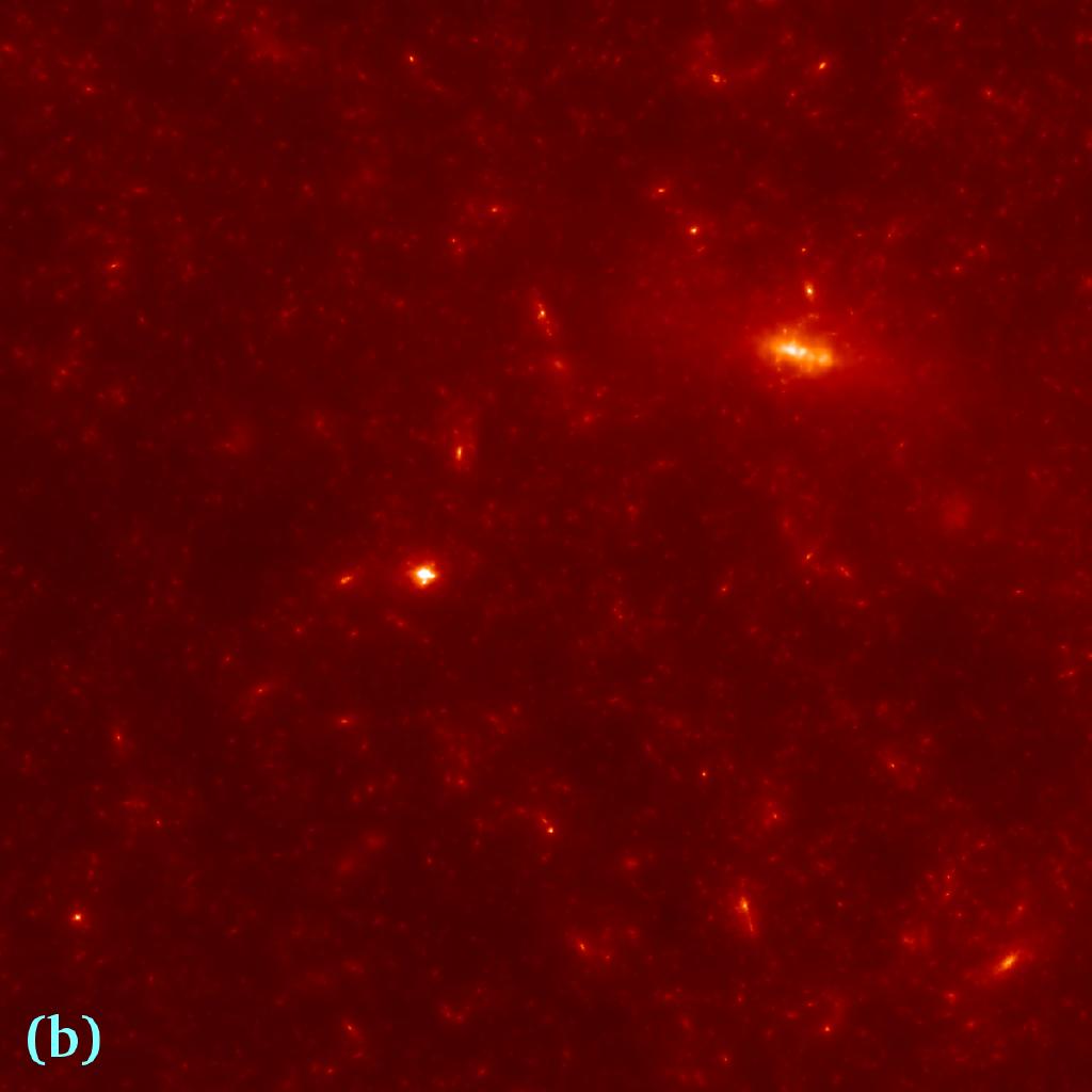
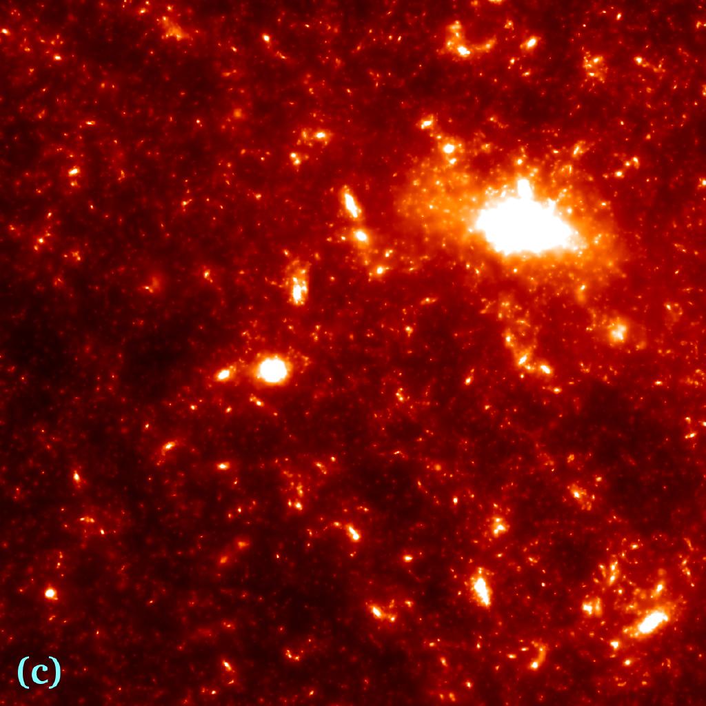
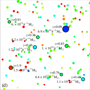

Figures 1, 2, and 3 show simulated convergence maps. The field shown in these examples is only a small fraction () of the full map that we simulated. The latter is too large to be displayed in sufficient detail. This particular field was chosen because it has a prominent mass concentration at upper right that is large enough to be detected in all the cases we investigate. This halo is at redshift and has a virial mass . Thus it represents a galaxy cluster similar to the Coma cluster. For this reason, the field is not typical. From our Millennium Simulation data, we find that there is only a 3% probability for a random field this size to contain a halo more massive than .
The second largest mass concentration visible in the field (at lower left) is at redshift and has a mass of . This is also a relatively unusual event. From our data, we expect one halo with and per square degree, corresponding to a 12% probability for a field. There are three more halos with masses above visible. The most prominent of these (left centre) is at redshift and has a mass of . On average, we expect about two such clusters in each field.
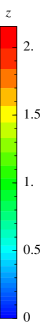
The three convergence maps in Fig. 1 are made without smoothing or added noise in order to illustrate the dependence on the redshift distribution of the sources. The map at top left gives the expected convergence distribution (at resolution) for sources at , representing the case of high-redshift 21-cm lensing. The map at top right uses the same colour table but a different source redshift distribution, that appropriate for an optimistic space-based galaxy survey. The principal impression in comparing the two is that there is much less structure in the ‘galaxy’ map. This reflects the lowering of the overall amplitude caused by the smaller source distances in the galaxy case. Averaged over the full area, the rms value of is 0.11 in the 21-cm map, but only 0.03 in the galaxy map (see Tab. 1 for a summary of the statistical properties of our simulated maps). The map at lower left repeats the galaxy map, but now the contrast is enhanced by a factor of 11/3 so that the colour range matches that of the 21-cm map. Displayed in this way, the two maps look similar. Nearby objects such as the most massive cluster appear stronger in the galaxy map, whereas more distant objects appear stronger in the 21-cm map. There are a few large structures that appear in the 21-cm map, but are absent from the galaxy map. These are objects that lie beyond the redshifts assumed for the galaxies. In particular, the large mass concentration at is clearly visible in the 21-cm map, but is virtually absent in the galaxy map. For the reader’s orientation, the lower right map indicates masses and redshifts for all halos in the field with .
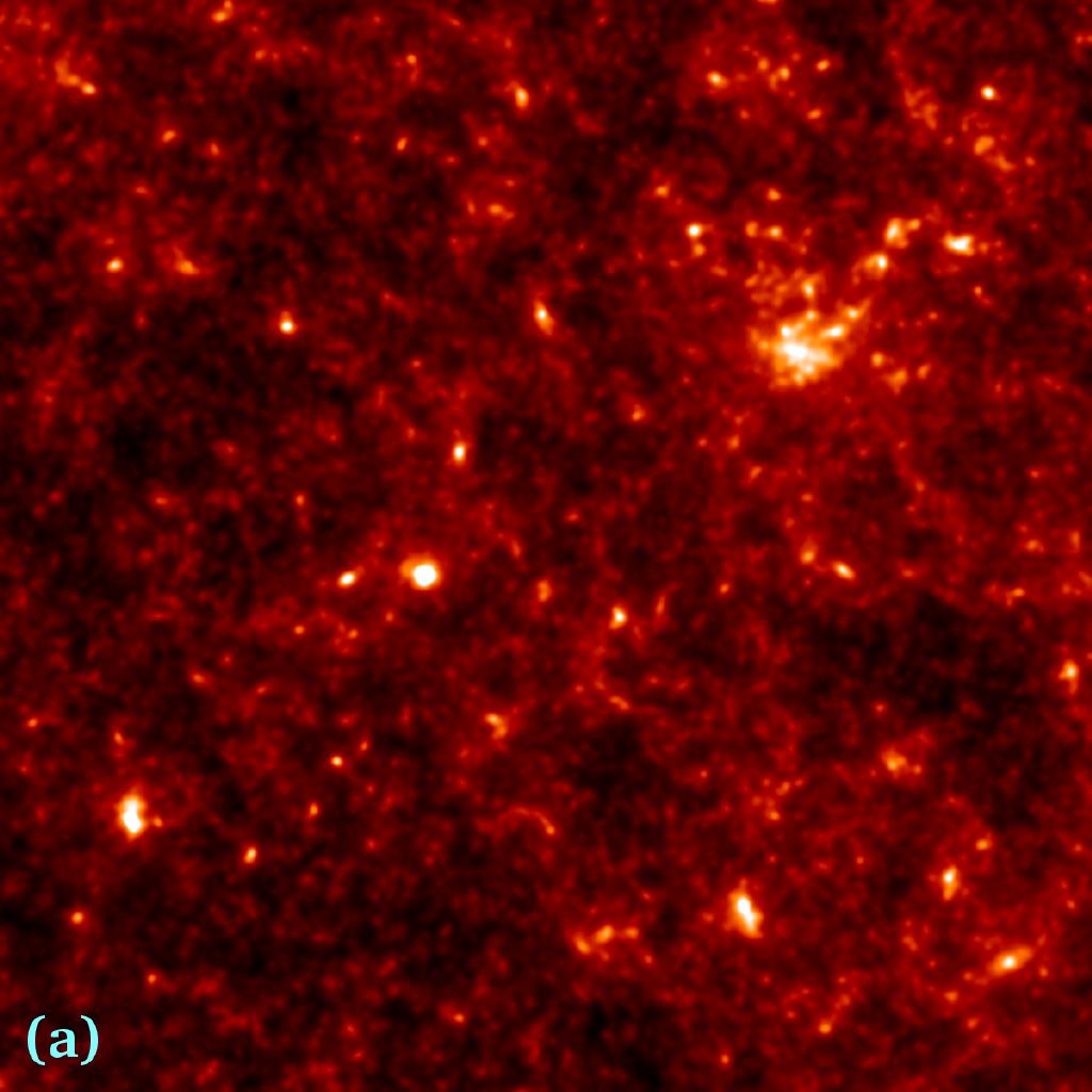
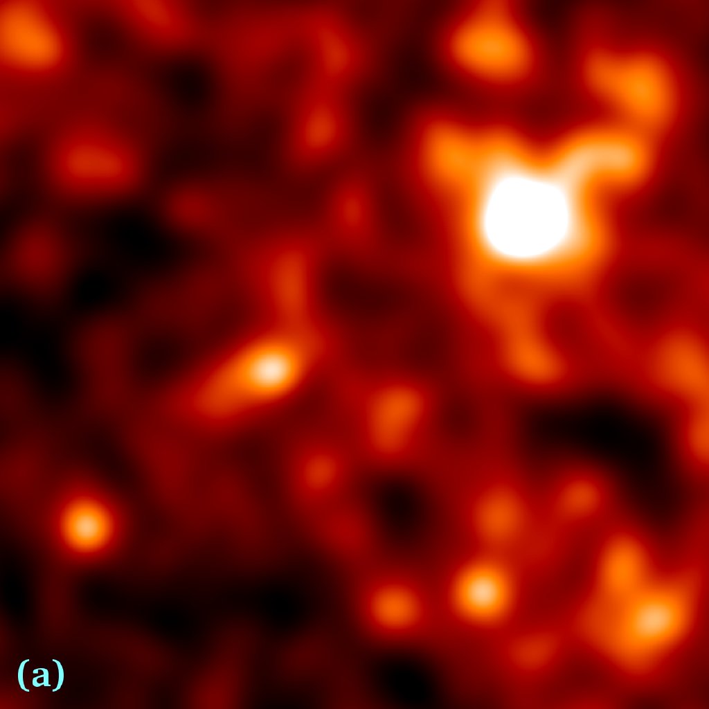
The two maps in Fig. 2 illustrate expectations for 21-cm lensing reconstructions based on a (futuristic) radio telescope with a Gaussian beam of width (corresponding to baselines ). The left image includes beam-smearing but excludes noise. A comparison with the map at the top left of Fig. 1 shows that very little detail is lost, and over the full area the rms value of is reduced by only 9% to 0.098. The right image also includes noise assuming the irreducible level expected for observations with the optimal band width for a telescope beam of this size (). This has virtually no effect on the image, demonstrating that such a (very large) telescope could produce high resolution mass maps with very high fidelity. All structures with (these are indicated in Fig. 1d) can be clearly identified out to high redshift, and even many smaller halos down to masses are visible. The signal-to-noise at the scale of the beam is very high even in low density regions, so substantial departures from optimal conditions could be tolerated without significant degradation of the resulting maps.
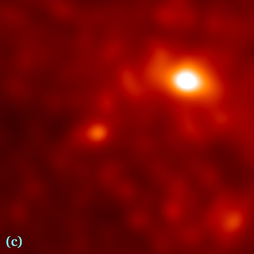
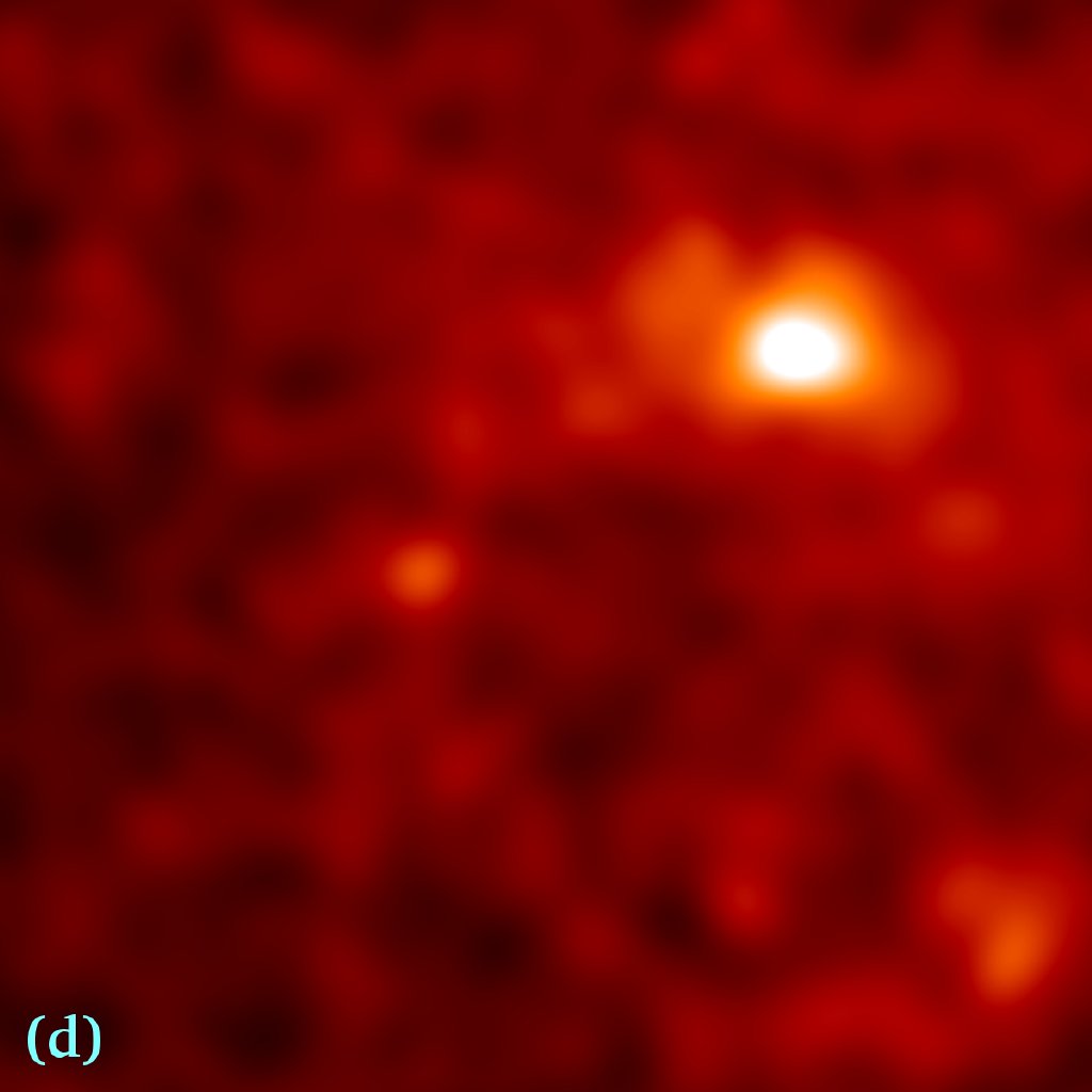
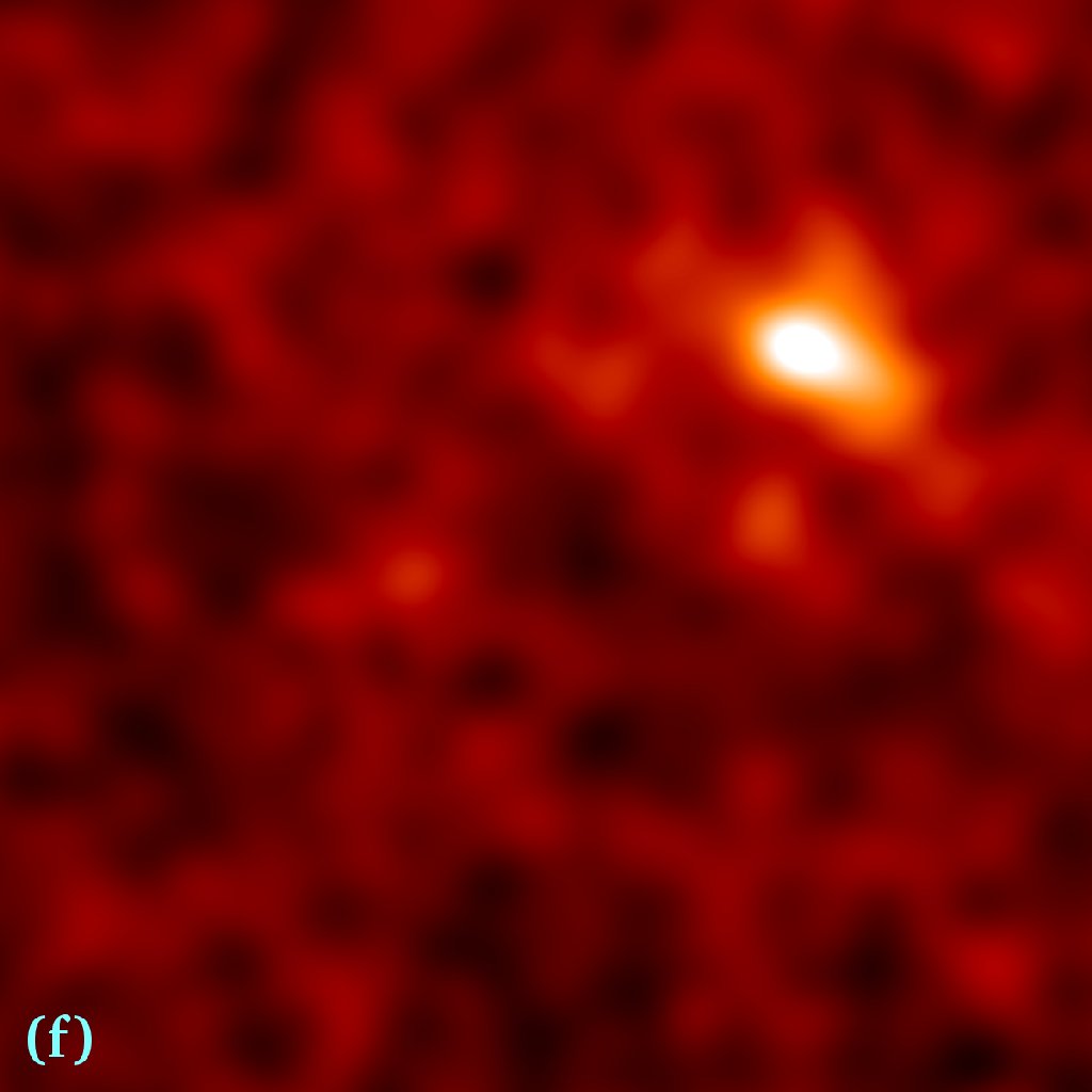
Figure 3 shows maps smoothed with a Gaussian of width . The colour scale is the same in all of them and differs from those of Fig. 1 an Fig. 2. Now, the resolution is similar to that obtainable with the planned Square Kilometer Array (Metcalf & White2007). The top two images are for sources at with no noise (left) and with noise at the irreducible level expected for observations at the optimal bandwidth for this beam-size (right). Again the fidelity of the image is high (although some differences can be seen in low areas), and many of the more massive halos indicated in Fig. 1d are detected individually. The middle row of maps are for our optimistic space-based galaxy lensing case, again without and with noise, while the bottom row gives the corresponding maps for our optimistic ground-based survey parameters. As at higher resolution, one is struck by how little structure is visible in these maps compared to the 21-cm case. The rms value of over the full field is smaller by factors of 3 and 4 in the space- and ground-based galaxy cases in comparison with the 21-cm case (see Table 1).
The fidelity of the ‘observed’ (i.e. noisy) maps is low in the galaxy lensing cases. A few of the structures seen in the noiseless maps are still visible in their noisy counterparts, in particular the largest object, but many of the low-amplitude peaks in these maps are due to noise. In effect, only the large cluster at is unambiguously detected for both surveys, while the two halos at also stand out above the noise in the ‘space-based’ map. The larger halo at remains unseen. The fidelity of these maps could be improved by increasing the smoothing length, but this would be at the expense of losing all the individual halos. In practice, an adaptive smoothing method such as a maximum entropy scheme would probably be used in order to remove low-significance features. This would leave rather little structure visible in our patch, only the highest peak in the ‘ground-based’ case. Only a few percent of fields this size would contain an object massive enough to be detected with high significance in a survey with these parameters. This limitation is quite evident in current ground-based lensing surveys (Semboloni et al. 2006; Bacon, Refregier & Ellis 2000; Kaiser, Wilson, & Luppino 2000; Van Waerbeke et al. 2000; Wittman et al. 2000).
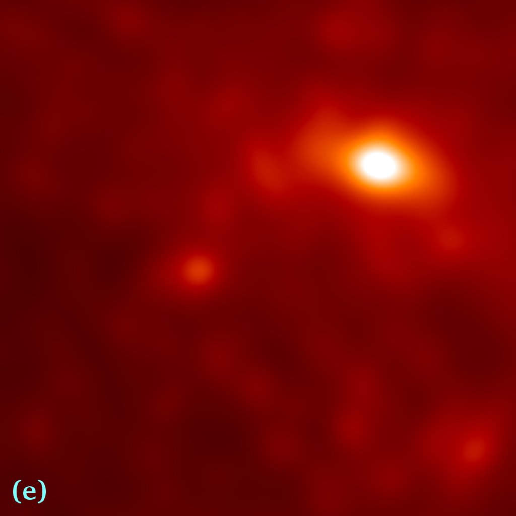
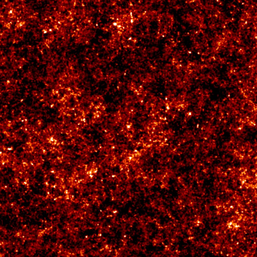
In order to give a better impression of the reconstruction capabilities of a radio telescope such as SKA, Fig. 4 shows the map of Fig. 3b expanded to show a field. (Note that this is still only 1/4 of the full field we simulated.) Current plans for the SKA should enable this resolution to be reached using the dense ‘core’ array, but the noise level in the convergence map will depend on the way in which reionisation proceeds. If the number density of ionised bubbles is large and they persist for a significant fraction of the redshift range expected for SKA () then noise levels nearly this good can be obtained in 90 days of integration time. A more pessimistic scenario is that reionisation happens very suddenly and nearly uniformly. Even if this is the case, and reionisation occurs near , moderate fidelity maps at resolution should be possible and the same noise levels as in Fig. 3 should be attainable but on scales. In the latter case, SKA maps will be more noisy than Fig. 3 after 90 days of integration, although still of much higher fidelity than galaxy-based maps.
The conclusion of this section is that galaxy lensing surveys do not provide sufficient signal-to-noise to image any but the most massive individual dark matter structures, but that a very large radio telescope could, in principle, provide high-resolution, high-fidelity images of the cosmic mass distribution in which the halos of individual massive galaxies and galaxy groups are visible.
4.2 Pixel distributions
Another useful way to represent the information in our simulated maps is to plot the probability density function for the convergence, , in the different cases. For this we can use the full degree field, rather than the smaller subfields discussed in section 4.1. Quantitative statistics for all these distributions are given in Table 1.
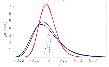
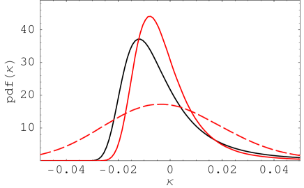
Figure 5 shows the results for sources at , as appropriate for pregalactic HI. This confirms quantitatively our previous conclusion that the irreducible noise has very little effect on the maps. Indeed, its effects are not even visible for a beam, and they are still small for . This just reflects the fact that the pdfs for the noise are much narrower than those for the signal, as illustrated in Fig. 5. Note that the narrower noise pdf is associated with the higher resolution, higher amplitude signal pdf.
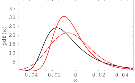
Figure 6 gives corresponding results for sources with the redshift distribution appropriate to a space-based galaxy lensing survey. Note that the scale has changed from Fig. 5, reflecting the substantially lower amplitude of fluctuations in in this case. For reconstructions with a beam of width , the noise expected in such a survey has a strong effect on . The low tail of the observed distribution is practically all due to noise, and the shape of distribution is largely lost. Estimating the skewness or kurtosis of the underlying distribution would clearly require a very good understanding of the properties of the noise.
The corresponding pdfs for the source redshift distribution and noise appropriate to a ground-based galaxy survey are shown in Fig. 7. Here the noise destroys almost all of the information in the original pdf. With a large amount of data and with good knowledge of the systematics one can recover the variance accurately, but determination of higher moments would be extremely challenging.
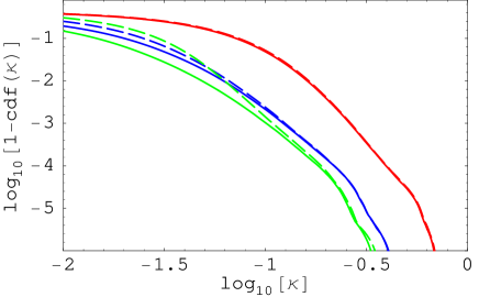
Even when the noise is high compared to the dispersion in , it is still possible to measure the number density of very high mass objects. Figure 8 illustrates this point by plotting the high tails of the cumulative distribution functions of . The noise has relatively little effect on these distributions for , even for the ground-based galaxy survey case. Such high values have a probability of around corresponding to of order one object per square degree on the sky. For our space-based survey parameters, the noise becomes unimportant for , corresponding to roughly 100 objects per square degree.
| Survey | ||||||
|---|---|---|---|---|---|---|
| 21-cm, | 1″ | - | 0.11 | 1.73 | -0.079 | 0.049 |
| 6″ | - | 0.098 | 1.35 | -0.071 | 0.046 | |
| 6″ | 0.0042 | 0.098 | 1.34 | -0.071 | 0.046 | |
| 1′ | - | 0.058 | 0.52 | -0.044 | 0.031 | |
| 1′ | 0.014 | 0.060 | 0.47 | -0.045 | 0.032 | |
| space-based, | 1″ | - | 0.030 | 3.95 | -0.020 | 0.007 |
| , | 1′ | - | 0.018 | 1.99 | -0.014 | 0.006 |
| 1′ | 0.012 | 0.022 | 1.09 | -0.017 | 0.010 | |
| ground-based, | 1″ | - | 0.021 | 4.61 | -0.014 | 0.005 |
| , | 1′ | - | 0.014 | 2.49 | -0.011 | 0.004 |
| 1′ | 0.02 | 0.024 | 0.31 | -0.018 | 0.014 |
5 conclusion
The noise in a mass map constructed using gravitational lensing of the high-redshift HI distribution is expected to be much smaller than the signal. In addition, the signal-to-noise increases with the resolution of the map. It should thus be possible to make high-resolution, high-fidelity images of the dark matter distribution in which the dark halos of individual galaxies and galaxy groups are visible. For example, a very large future telescope with baselines may eventually allow us to detect halos with virial masses out to redshift (Metcalf & White 2007). Such detailed observations will provide a very direct and accurate test for structure-formation models. Even with an SKA-like telescope, halos with should be clearly detected out to high redshift. This contrasts strongly with mass maps constructed using gravitational lensing of distant galaxies, where high fidelity is only achievable for angular smoothings so large that all but the nearest and most massive individual objects are lost.
Our estimates of the irreducible noise are based on a convergence estimator that is not necessarily optimal. It may therefore be possible to achieve smaller ‘irreducible’ noise levels than we quote. In practice, however, it is likely that other sources of error will dominate the overall budget, for example, the error introduced by incomplete foreground subtraction (see Furlanetto et al. 2006, for a review). For most purposes, imaging the surface density does not require reaching the irreducible noise limit; the predicted signal is large enough to accommodate a noise level many times the irreducible value. In addition, the noise within a patch of area goes down like while the density fluctuations go down roughly like , so even if the noise is too large to map the surface density on the scale of a single beam, a high-fidelity map with larger smoothing can still be constructed (as in the galaxy lensing case). The Square Kilometer Array in its currently proposed configuration should be able to map the mass distribution on arcminute scales with moderate to high fidelity if reionisation is not completed too early (Metcalf & White 2007). The optimal bandwidth for observing lensing is while the signal-to-noise for mapping the pregalactic HI at the same angular scales is maximal at larger bandwidths . Lensing benefits from the stacking of many narrow redshift slices even if they are individually noise dominated while the temperature fluctuations themselves get diluted (Metcalf & White 2007). To reach scales of a few arcseconds as discussed here will require a larger telescope with dense sampling. Given the narrower science goals, this may be achievable with simpler and cheaper antennas.
While high-resolution images of the cosmic mass distribution would be a unique product of observations of 21-cm lensing, they are not the only reason to carry out such studies. If enough of the sky can be surveyed, cosmological parameters such as the density of dark energy and its evolution with redshift can be measured with much higher accuracy by a combination of 21-cm lensing with galaxy lensing than they can by galaxy lensing alone or indeed by any other method proposed so far (Metcalf & White 2007). The baseline configuration of SKA may be powerful enough to achieve much of this improvement if problems with foregrounds can be overcome.
References
- [Bacon, Refregier, & Ellis 2000] Bacon, D. J., Refregier, A. R., & Ellis, R. S. 2000, MNRAS, 318, 625
- [Furlanetto, Oh, & Briggs 2006] Furlanetto, S., Oh, S. P., & Briggs, F. 2006, Phys.Rept., 433, 181
- [Hilbert, White, Hartlap, & Schneider 2007] Hilbert, S., White, S. D. M., Hartlap, J., & Schneider, P. 2007, MNRAS, 382, 121
- [Kaiser, Wilson, & Luppino 2000] Kaiser, N., Wilson, G., & Luppino, G. A. 2000, ArXiv Astrophysics e-prints, astro-ph/0003338
- [Massey et al. 2007a] Massey, R. et al. 2007a, ApJS, 172,239
- [Massey et al. 2007b] —. 2007b, Nature, 445, 286
- [Metcalf & White 2007] Metcalf, R. & White, S. 2007, MNRAS, 381, 447
- [Semboloni, Mellier, van Waerbeke, Hoekstra, Tereno, Benabed, Gwyn, Fu, Hudson, Maoli, & Parker 2006] Semboloni, E., et al. 2006, AAP, 452, 51
- [Smail, Ellis, & Fitchett 1994] Smail, I., Ellis, R. S., & Fitchett, M. J. 1994, MNRAS, 270, 245
- [Springel, White, Jenkins, Frenk, Yoshida, Gao, Navarro, Thacker, Croton, Helly, Peacock, Cole, Thomas, Couchman, Evrard, Colberg, & Pearce 2005] Springel, V., et al. 2005, Nature, 435, 629
- [Vale & White 2003] Vale, C. & White, M. 2003, ApJ, 592, 699
- [van Waerbeke 2000] van Waerbeke, L. 2000, MNRAS, 313, 524
- [Van Waerbeke, Mellier, Erben, Cuillandre, Bernardeau, Maoli, Bertin, Mc Cracken, Le Fèvre, Fort, Dantel-Fort, Jain, & Schneider 2000] Van Waerbeke, L., Mellier, Y., Erben, T., Cuillandre, J. C., et al. 2000, AAP, 358, 30
- [Wittman, Tyson, Kirkman, Dell’Antonio, & Bernstein 2000] Wittman, D. M., Tyson, J. A., Kirkman, D., Dell’Antonio, I., & Bernstein, G. 2000, Nature, 405, 143
- [Zahn & Zaldarriaga 2006] Zahn, O. & Zaldarriaga, M. 2006, ApJ, 653, 922
- [Zwicky 1933] Zwicky, F. 1933, Helvetica Physica Acta, 6, 110
- [Zaldarriaga, Furlanetto, & Hernquist 2004] Zaldarriaga, M., Furlanetto, S. R., & Hernquist, L. 2004, ApJ, 608, 622