On the Magnetic Prandtl Number Behavior
of Accretion Disks

Abstract

We investigate the behavior of the magnetic Prandtl number (ratio of microscopic viscosity to resistivity) for accretion sources. Generally this number is very small in standard accretion disk models, but can become larger than unity within $\sim 50$ Schwarzschild radii of the central mass. Recent numerical investigations suggest a marked dependence of the level of MHD turbulence on the value of the Prandtl number. Hence, black hole and neutron star accretors, i.e. compact X-ray sources, are affected. The astrophysical consequences of this could be significant, including a possible route to understanding the mysterious state changes that have long characterized these sources.

1 Introduction

Magnetohydrodynamic (MHD) turbulence differs from ordinary hydrodynamic turbulence in at least one very important respect: whereas the latter generally has only one dissipative scale (viscous), MHD turbulence has two (viscous and resistive). This raises the question of whether the classical Kolmogorov picture, in which the large scale energetics of the turbulenct cascade is essentially independent of small scale dissipation physics, remains valid in MHD turbulence. And if it is not valid, what are some possible astrophysical consequences?

The dimensionless ratio of the kinematic viscosity $\nu$ to the electrical resistivity $\eta$ is known as the magnetic Prandtl number, ${\rm Pm}$. Balbus & Hawley (1998) suggested that even if both the viscous and resistive dissipation scales are very small, the saturation level of the MHD turbulence produced by the magnetorotational instability (MRI) should be sensitive to ${\rm Pm}$, at least in the neighborhood of ${\rm Pm}\simeq 1$. Their argument was as follows. If ${\rm Pm}\ll 1$, the resistive scale is much larger than the viscous scale. Assuming that the velocity fluctuations do not greatly exceed the Alfvénic fluctuations at the resistive scale, viscous stresses on the resistive scale would be small. This would mean that even if relatively large velocity gradients accompanied magnetic dissipation, these gradients would not produce stresses that would interfere with the dynamics of the field reconnection. Since Lorentz forces drive the MRI, the dissipation of the magnetic field is an important regulatory mechanism for the saturation level of the turbulence. On the other hand, if ${\rm Pm}\gg 1$, and the viscous scale were significantly larger than the resistive, then the resulting dynamical stresses would likely be relatively large when the magnetic field is dissipated at the small resistive scale. (This assumes that significant velocity fluctuations accompany small scale reconnection. Such fluctuations would be heavily damped at the resistive scale, and any reconnection would have to be very slow.) These stresses would then interfere with the field reconnection and dissipation, leading to a build-up of magnetic energy that cascades upwards, back to larger scales (Brandenburg 2001).

Balbus & Hawley (1998) were motivated by the possibility that the turbulent properties of accretion disks might be different in the regimes ${\rm Pm}\gg 1$ and ${\rm Pm}\ll 1$. At the time, direct numerical simulation of flows with different Prandtl numbers was very difficult, and these authors attempted only the crudest of tests by varying the level of artificial viscosity in the ZEUS MHD code at fixed resolution. These preliminary experiments did, however, show a higher level of saturation for a larger viscosity. Since this is an example in which increasing a dissipation coefficient actually raised the level of turbulent activity, it was a noteworthy result.

A decade on, it is possible to do much better. There is a definite sensitivity to ${\rm Pm}$ in numerical simulations of MHD turbulence. A ${\rm Pm}$ dependence has been observed for a number of years now in stirred magnetic turbulence (Schekochihin et al. 2004, 2005). For example, fluctuation dynamos at large Pm were found numerically by Schekochihin et al. (2004), but until recently there was some question as to whether a low ${\rm Pm}$ fluctuation dynamo even existed; this has now been answered affirmatively (Iskakov et al. 2007; Schekochihin et al. 2007). For astrophysical accretion flows, MRI calculations are of direct interest, and the last year has seen the first ${\rm Pm}$ studies in “shearing box” simulations. Zero mean field calculations have been carried out by Fromang et al. (2007), while Lesur & Longaretti (2007) studied a mean vertical field. In the latter investigation, the radial-azimuthal component of the stress tensor behaved linearly over the range $0.12<{\rm Pm}<8$ with no apparent sign of approaching an asymptote (Iskakov et al. [2007] did, however, appear to be reaching saturation levels in some of their driven turbulence runs). With extensive numerical evidence of a ${\rm Pm}$ dependence in MHD turbulence, a natural question to raise is what is the behavior of ${\rm Pm}$ in classical accretion disk models? In particular, is there a transition from ${\rm Pm}\ll 1$ to ${\rm Pm}\gg 1$ in phenomenological models that have been used to model AGN and compact X-ray sources?

In this paper, we examine the magnetic Prandtl number behavior of classical $\alpha$ models. In fact, the only feature of these models that is important for our purposes is that the free energy of differential rotation be locally dissipated—a variable $\alpha$ parameter, for example, would hardly change our conclusions at all. Throughout the regime of interest, the disk is fully ionized and collision dominated (see §2 below), so that the Spitzer (1962) values for the resistivity and viscosity are appropriate. Our principal finding is that generally ${\rm Pm}\ll 1$ nearly everywhere in classical $\alpha$ models, with one robust and important exception: on scales less than $\sim 100$ Schwarzschild radii in black hole and neutron star disks. It is extremely tempting to associate this Prandtl number transition with a physical transition in the properties of the accretion flow, here motivated by “first principle” physics. Further discussion of this point is presented below.

An outline of the paper is as follows. §2 presents preliminary estimates of important parameter regimes. §3 is the heart of the paper, in which we calculate the behavior of ${\rm Pm}$ in classical $\alpha$ disk models. Transitions from low ${\rm Pm}$ to high $Pm$ regions occur only in disks around black holes and neutron stars. Finally, §4 is a discussion of the possible astrophysical consequences of having both high ${\rm Pm}$ and low ${\rm Pm}$ regions in the same disk. It is argued that high and low X-ray states (e.g. McClintock & Remillard 2006) may be related to an unstable interface between ${\rm Pm}<1$ and ${\rm Pm}>1$ regions of the disk.

2 Preliminaries

The magnetic Prandtl number is not a standard parameter of accretion theory, so let us begin with a brief orientation in the temperature-density parameter space. Throughout this work, the fiducial disk plasma is taken to be a mixture of 90% hydrogen and 10% helium (by number). Following the discussion in Spitzer (pp. 138-9), we estimate an averaged resistivity of such a fully ionized gas as

$$\eta={5.55\times 10^{11}\ln\Lambda_{\rm e\,H}\over T^{3/2}}\ {\rm cm}^{2}\ {\rm s}^{-1},$$ (1)

where $T$ is the temperature in Kelvins, and $\Lambda_{\rm e\,H}$ is the Coulomb logarithm for electron-proton scattering. (Modifications in the logarithm due to electron-helium scattering, here a minor effect, are ignored.)

The kinematic viscosity of the same gas is estimated to be

$$\nu={1.6\times 10^{-15}T^{5/2}\over\rho\ln\Lambda_{\rm H\,H}}\ {\rm cm}^{2}\ {\rm s}^{-1},$$ (2)

where $\rho$ is the mass density and $\ln\Lambda_{\rm H\,H}$ is the Coulomb logarithm for scattering of protons by protons. (See Appendix for a derivation of these results and a discussion of the Coulomb logarithms.) This gives a magnetic Prandtl number of

$${\rm Pm}=2.9\times 10^{-27}{T^{4}\over\rho\ln\Lambda_{\rm e\,H}\ln\Lambda_{\rm H\,H}}.$$ (3)

The two logarithms differ from one another for temperatures in excess of $4.2\times 10^{5}$ K (see Appendix). If $l$ is the product of the two Coulomb logarithms normalized to a nominal value of 40,

$${\rm Pm}=\left(T\over 4.2\times 10^{6}\,{\rm K}\right)^{4}\left(10^{22}\,{\rm cm}^{-3}\over l\ n_{H}\right)=\left(T\over 4.2\times 10^{4}\,{\rm K}\right)^{4}\left(10^{14}\,{\rm cm}^{-3}\over l\ n_{H}\right),$$ (4)

where $n_{H}$ is the number density of hydrogen atoms. The two last forms that are given for ${\rm Pm}$ are convenient for applications to a $10\,M_{\odot}$ (binary) and $10^{8}\,M_{\odot}$ (AGN) black hole, respectively.

Finally, it is required to justify quantitatively the statement in the Introduction that the disk plasma is collisional near the transtion point ${\rm Pm}=1$. We shall refer to a plasma as “dilute” (as opposed to collisional) if the product of the ion cyclotron frequency $\omega_{ci}$ and the ion-ion collision time $t_{ci}$ is greater than one. The proton cyclotron frequency may be written

$$\omega_{ci}=8.6\times 10^{-4}\left(n_{H}T\over\beta\right)^{1/2},$$ (5)

where we have introduced the plasma $\beta$ parameter, the ratio of the gas to magnetic pressure. For a gas of cosmic abundances,

$$\beta=2.3\left(8\pi n_{H}kT\over B^{2}\right).$$ (6)

In a dilute plasma, it is not appropriate to use the Spitzer (1962) form of the viscosity, as we have done above, hence we need a numerical estimate of $\omega_{ci}t_{ci}$. (It is also not strictly correct to use the Spitzer resistivity, but the correction here is relatively minor.) Following the prescription set forth in the Appendix (divide the nominal proton-proton collision time by a factor of 1.5 to include the effects of proton-helium collisons), we obtain

$$\left(\omega_{ci}t_{ci}\right)^{2}\simeq 9\times 10^{-7}{T^{4}\over n_{H}\beta}.$$ (7)

where we have taken the relevant Coulomb logarithm to be 7. This should be compared directly to ${\rm Pm}\simeq 3\times 10^{-5}T^{4}/n_{H}$ from equation (3). For a given value of $\beta$, the temperature and density dependence of $\omega_{ci}^{2}t_{ci}^{2}$ and ${\rm Pm}$ are the same. What is more, we are concerned in this work with weakly magnetized plasmas, $\beta>1$, and generally $\beta\gg 1$. Therefore, at the threshold ${\rm Pm}=1$, the plasma is never dilute, and the collisional regime is valid. Note, however, that once into the large ${\rm Pm}$ regime, substantial heating and magnetic field growth may lead to a dilute plasma phase, or perhaps even to a fully collisionless phase in which the fluid approximation itself breaks down.

3 Analysis

Our goal is a simple one: we wish to follow the behavior of ${\rm Pm}$ with disk radius in a standard $\alpha$ model, in effect testing such models for self-consistency. If most of the energy extracted from differential rotation is locally dissipated, the basic $\alpha$ scalings are probably robust. This is particularly true if the problem is framed to minimize any possible explicit dependence upon $\alpha$ of the temperature and density, as we have done. Then, even if in real disks it is not a very good approximation to treat $\alpha$ as a constant, its variability is not crucially important for the scaling laws.

3.1 Pm behavior in $\alpha$ models

Our starting point is the Kramers opacity disk model of Frank, King, and Raine (2002). The density in the midplane is

$$\rho=3.1\times 10^{-8}\alpha^{-7/10}{\dot{M}_{16}}^{11/20}(M/M_{\odot})^{5/8}{R_{10}}^{-15/8}q^{11/20}\ {\rm gm}\,{\rm cm}^{-3},$$ (8)

where ${\dot{M}_{16}}$ is the mass accretion rate in units of $10^{16}$ g s^-1, $M/M_{\odot}$ is the central mass in solar units, $R_{10}$ is the cylindrical radius $R$ in units of $10^{10}$ cm., and $q=1-(R_{*}/R)^{1/2}$. The quantity $R_{*}$ is a fiducial radius at which the stress is taken to vanish (the “inner edge”), but in practice we shall assume that $R\gg R_{*}$, and hence that $q$ is unity. The midplane temperature is given by Frank et al. (2002) as

$$T=1.4\times 10^{4}\alpha^{-1/5}{\dot{M}_{16}}^{3/10}(M/M_{\odot})^{1/4}{R_{10}}^{-3/4}q^{3/10}\ {\rm K}.$$ (9)

This leads to a Prandtl number of

$${\rm Pm}=9.0\times 10^{-5}l^{-1}\alpha^{1/10}{\dot{M}_{16}}^{13/20}(M/M_{\odot})^{3/8}{R_{10}}^{-9/8}q^{13/20}.$$ (10)

Typical disk Prandtl numbers are therefore very small, and insensitive to scaling with $\alpha$. Transitions from low to high ${\rm Pm}$, if they occur at all, will occur in the inner disk regions.

Let us calculate $R_{cr}$, the critical radius at which ${\rm Pm}=1$. Here, it will suffice to set $q=1$ ($R\gg R_{*}$); a more accurate numerical calculation (described below) certainly justifies this. With ${\rm Pm}=1$, we find

$$R_{cr}=2.5\times 10^{6}\ l^{-8/9}\alpha^{-4/45}{\dot{M}_{16}}^{26/45}(M/M_{\odot})^{1/3}\ {\rm cm}.$$ (11)

The region of interest is evidently on scales of tens of Schwarzschild radii ($R_{S}$). With $R_{S}=2GM/c^{2}$, this becomes

$${R_{cr}\over R_{S}}=8.5\alpha^{-4/45}{\dot{M}_{16}}^{26/45}(M/M_{\odot})^{-2/3}l^{-8/9}.$$ (12)

Our final step is to scale the mass accretion rate with $M$. If we assume that the source luminosity $L$ is a fraction $\epsilon$ of ${\dot{M}}c^{2}$ and a fraction $\delta$ of the Eddington luminosity

$$L_{Edd}=1.26\times 10^{38}(M/M_{\odot})\ {\rm erg}\ {\rm s}^{-1},$$

then

$${R_{cr}\over R_{S}}=59\left(\alpha_{-2}M/M_{\odot}\right)^{-4/45}(\delta/\epsilon)^{26/45}l^{-8/9}$$ (13)

where $\alpha_{-2}$ is $\alpha$ in units of 0.01. The ratio $\delta/\epsilon$ is just the mass accretion rate measured in units of the Eddington value $\dot{M}_{Edd}=L_{Edd}/c^{2}$. This shows that the critical radius at which the Prandtl number transition occurs, when measured in units of $R_{S}$, is remarkably insensitive to the central mass. In general we find that $R_{cr}$ varies roughly between 10 and 100 $R_{S}$. In principle, the low ${\rm Pm}$ region could in some cases extend all the way down to $2-3R_{S}$, particularly for larger AGN masses. Iron line observations of, for example, the well-studied Seyfert galaxy MCG–60–30–15, (Fabian et al. 2002) suggest the presence of an ordinary Keplerian-like disk down to $3R_{S}$, and the ${\rm Pm}$ transition hypothesis must accommodate this: no transition should also be a possibility.

3.2 ${\rm Pm}$ behavior in numerical $\alpha$ models

The result of the previous section neglects radiation pressure and electron scattering contributions to the opacity. In particular, the radiation to gas pressure ratio is easily calculated. With $q=1$,

$${P_{rad}\over P_{gas}}=5\times 10^{-3}\alpha^{1/10}{\dot{M}_{16}}^{7/20}(M/M_{\odot})^{1/8}{R_{10}}^{-3/8}.$$ (14)

(This differs from equation [5.56] in Frank et al. [2002].) At $R=R_{cr}$,

$${P_{rad}\over P_{gas}}=0.16l^{1/3}\left({\alpha\delta\over\epsilon}{M\over M_{\odot}}\right)^{2/15}.$$ (15)

This varies between a $10\%$ and an order unity effect for applications of interest. To ensure that radiative corrections do not alter the basic conclusion of the existence of a crtical ${\rm Pm}$ transition radius under nominal conditions, we have adapted the disk code of Terquem & Papaloizou (1999) to construct more detailed $\alpha$ models. Both radiation pressure and electron scattering opacity were included. We find that the essential qualitative features of equation (13) remain intact, though radiative effects do alter the scalings somewhat. We focus on two central masses, one a source of $10M_{\odot}$ (representative of an X-ray binary), the other $10^{8}M_{\odot}$, which is representative of an AGN. The Prandtl number behavior for each of these cases for several different values of $\alpha$, but at a fixed accretion rate ($0.1\dot{M}_{Edd}$), is shown in figure (1). The two cases are very similar. Starting with a standard Keplerian $\alpha$ disk, these black hole accretion sources seem to make a transition from low ${\rm Pm}$ to high ${\rm Pm}$ at a typical value of $\sim 50R_{S}$.

Figures (2) and (3) show ${\rm Pm}$ plots as meridional slices. A central mass of $10M_{\odot}$ is assumed for figure (2), while figure (3) corresponds to $10^{8}M_{\odot}$. In each figure, the left and right diagrams correspond respectively to $\dot{M}/\dot{M}_{Edd}=0.001,1$. We have used $\alpha=0.05$. At higher accretion rates, the ${\rm Pm}>1$ region can be extensive; on the other hand, if ${\dot{M}}/\dot{M}_{Edd}$ is sufficiently small, the flow can have ${\rm Pm}<1$ down to the marginally stable orbit $R=3R_{S}$.

Figure 1: Behavior of ${\rm Pm}$ for $10M_{\odot}$ (left) and $10^{8}M_{\odot}$ (right) black holes for several different $\alpha$ values as a function of disk radius $R/R_{S}$, where $R_{S}$ is the Schwarzschild radius. The accretion rate is taken to be $0.1\dot{M}_{Edd}$. Calculations were carried out using the code of Terquem & Papaloizou (1999) including radiation pressure and electron scattering corrections to the opacity. Note the insensitivity of the results to both $\alpha$ and the central mass.

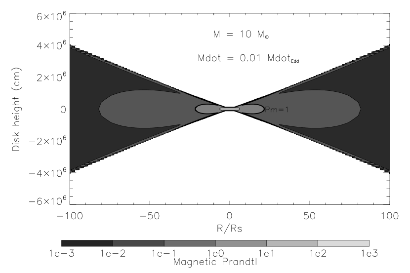
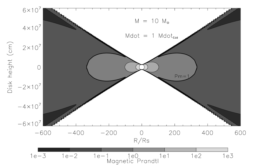
Figure 2: Regions of ${\rm Pm}$ for a $10M_{\odot}$ black hole accretion disk. Left diagram corresponds to $\dot{M}=0.01\dot{M}_{Edd}$, right to $\dot{M}=\dot{M}_{Edd}$. In both cases, $\alpha=0.05$. At large accretion rates, the high ${\rm Pm}$ regions can be quite extended. (Note change of radial scale.)

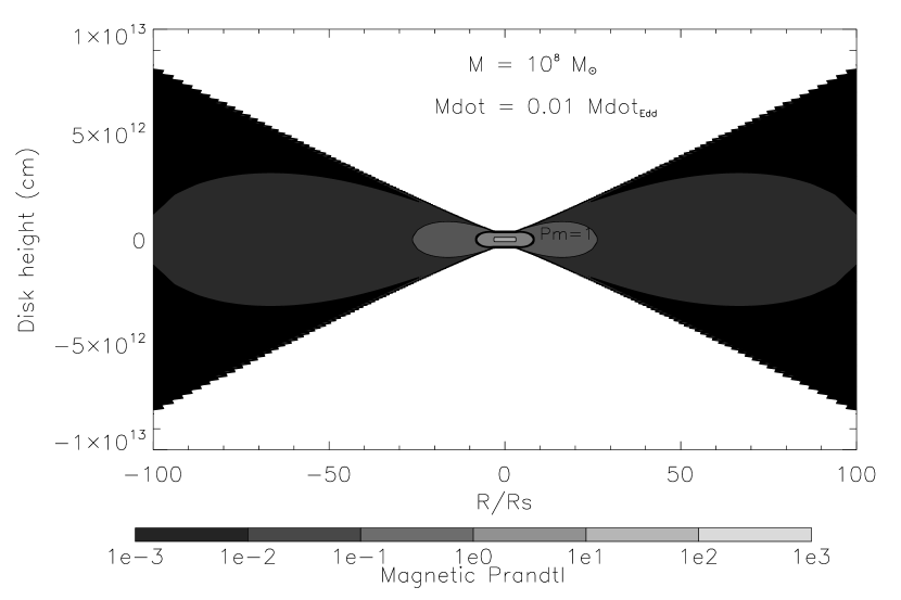
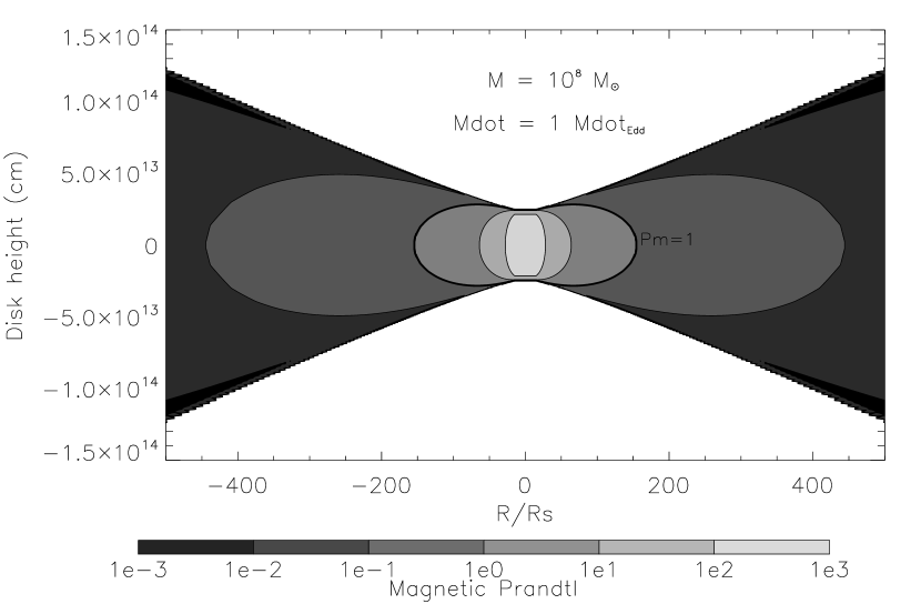
Figure 3: Regions of ${\rm Pm}$ for a $10^{8}M_{\odot}$ black hole accretion disk. Left diagram corresponds to $\dot{M}=0.01\dot{M}_{Edd}$, right to $\dot{M}=\dot{M}_{Edd}$. In both cases, $\alpha=0.05$. The high ${\rm Pm}$ regime is very limited in the low $\dot{M}$ case on the left. (Note change of radial scale.)

4 Discussion

The findings of the previous section show that if $\alpha$ models are even qualitatively correct in their scalings, only black holes and neutron star accretion disks, i.e., classical X-ray sources, will have regions with ${\rm Pm}<1$ and ${\rm Pm}>1$. If, as we would argue, there is a physical difference in the saturated state of MHD turbulence in these two regimes, it should be reflected in the astrophysical behavior manifested by X-ray sources. We tentatively suggest that the principal hard high states and low soft states associated with these sources is related respectively to the relative radiative dominance of the ${\rm Pm}>1$ and ${\rm Pm}<1$ accretion regions. In this discussion we will outline arguments that are suggestive, but as yet far from conclusive, of this. They are meant to spur further numerical investigation in what could prove to be an interesting direction.

The results of several independent numerical simulations of MHD turbulence, both forced and shear-driven, appear to indicate that if ${\rm Pm}>1$, field dissipation becomes more inefficient, apparently because viscous stresses make the resistive scale less accessible (Fromang et al. 2007, Lesur & Longaretti 2007, Iskakov et al. 2007). If field dissipation is inefficient, the most likely scenario is that the field will initially build up on the viscous scale, but ultimately cascade upward to larger scales (Brandenburg, 2001). In a disk, the growing magnetic field would drive the MRI more vigorously until ultimately — and “ultimately” may in fact be rather rapid — the field is of order thermal. At this stage further MRI development is likely to be halted.

The effective absence of resistivity of course does not mean that dissipation is absent; dissipative heating will still be present in the form of viscous heating. Note that the dominance of the resistive scale in ${\rm Pm}<1$ turbulence means that the electrons are directly heated (assuming that classical Spitzer resistivity applies), whereas the ions are directly heated in viscosity dominated ${\rm Pm}>1$ turbulence. The need for the dominance of ion heating in low luminosity black hole accretion is by no means a new idea (e.g. Narayan & Yi 1995), but placing it within the Prandtl number framework lends mutual support to this current work and to what has become the standard picture. In addition, the heating of a ${\rm Pm}>1$ magnetized plasma may be very vigorous—unlike ohmic resistivity, viscous thermalization does not destroy the current sources.

Conditions for a thermal runaway are present: at constant pressure, ${\rm Pm}\propto T^{5}$. Since ${\rm Pm}$ is an increasing function of temperature, a little heating would tip ${\rm Pm}\sim 1$ accretion towards the direction of ${\rm Pm}\gg 1$ accretion. This would mean yet greater heating, following the numerical lead that large Pm turbulence is characterized by greater fluctuation levels. But this argument works in both directions, cooling as well as heating. A formal boundary between high and low Prandlt number regions would, in this view, be unstable because of the dependence of Pm upon $T$. This can be investigated by direct simulation. We speculate that the ${\rm Pm}<1$ region is a standard $\alpha$ disk and responsible for soft thermal emission; the ${\rm Pm}>1$ region corresponds to lower density, hotter accretion. Although such a component has been regarded as essential for understanding the X-ray spectra of black hole accretion sources, the reason that a disk would suddenly make the transition from one type of flow to the other has always been unclear. Prandtl number considerations may make this transition less mysterious.

The unstable boundary between high and low Prandtl number flow marks a fundamental change in the accretion flow, leading to a distinct inner accretion zone that dominates the hard tail of the X-ray spectrum. A better understanding of the interface will help to establish whether it is involved with transitions from one state to another. In a subsequent publication, we will present a technique to make this problem tractable and predictive.

At this point the major gap in our scenario is the difference between the modest but rigorous numerical findings of a correlation between ${\rm Pm}$ with the amplitude of the turbulent stress, and the full blown thermal runaway that we envisage. That gap can begin to be filled with well-crafted numerical investigations of temperature-dependent dissipation coefficients in MRI turbulence. Little has yet been done along these lines, and it promises to be extremely challenging, particularly if the ideas presented here are qualitatively correct and a dilute or collisionless plasma appears. But preliminary investigations have already begun.

We end by noting that in the paper introducing the MRI to the astrophysical community (Balbus & Hawley 1991), two possible nonlinear resolutions were envisioned. In one the field was limited to subthermal strengths by vigorous dissipation; in the other it grew to thermal levels and became “stiff.” Subsequent numerical simulations seem to support the first outcome, but this may well have been because the codes used were not in the large ${\rm Pm}$ regime. Both scenarios might in fact be equally viable, the choice of direction being made by the Prandtl number of the turbulence.

Appendix: Collision time and viscosity estimates.

Spitzer (1962) defines a “deflection time” $t_{D}$ for a test particle (denoted by subscript $t$) of mass $m_{t}$, charge $Z_{t}$ (in units of $e$), and velocity $w_{t}$ to be scattered by Coulomb interactions by a population of field particles (denoted by subscript $f$) of number density $n_{f}$. It is given by

$$t_{D}(t\rightarrow f)={m_{t}^{2}w_{t}^{3}\over 8\pi n_{f}e^{4}Z_{t}^{2}Z_{f}^{2}\,F(l_{f}w_{t})\,\ln\Lambda_{tf}}.$$ (16)

Here,

$$l_{f}=\sqrt{m_{f}\over 2kT_{f}}$$ (17)

with $m_{f}$ and $T_{f}$ refering respectively to the mass and temperature of the field particles. The function $F(x)$ is

$$F(x)=\left(1-{1\over 2x^{2}}\right){\rm erf}(x)+{e^{-x^{2}}\over x\sqrt{\pi}}$$ (18)

where erf$(x)$ denotes the standard error function

$${\rm erf}(x)={2\over\sqrt{\pi}}\int_{0}^{x}e^{-s^{2}}\,ds.$$ (19)

The argument of the logarithm is

$$\Lambda_{tf}={1.5\over Z_{t}Z_{f}e^{3}}\,\left(k^{3}T_{t}^{2}T_{e}\over\pi n_{e}\right)^{1/2}$$ (20)

where $T_{t}$ and $T_{e}$ refer to the test particle and electron temperature, respecitvely, and $n_{e}$ is the electron density. When the test particles are electrons, then for temperatures in excess of $4.2\times 10^{5}$K, an additional factor of $(4.2\times 10^{5}/T_{e})^{1/2}$ appears in the expression for $\Lambda$ (a correction for quantum diffraction).

In what follows, we shall always take a single temperature ($T$) fluid, and set $w_{t}$ equal to the rms test particle velocity, i.e., $m_{t}w_{t}^{2}=3kT$. Then,

$$t_{D}(t\rightarrow f)={m_{t}^{1/2}(3kT)^{3/2}\over 8\pi n_{f}e^{4}Z_{t}^{2}Z_{f}^{2}\,F(\sqrt{3m_{f}/2m_{t}})\,\ln\Lambda_{tf}}.$$ (21)

and, with $n_{H}$ denoting hydrogen number density,

$$\Lambda_{tf}={1.5\over Z_{t}Z_{f}e^{3}}\,\left(k^{3}T^{3}\over\pi n_{e}\right)^{1/2}={1.239\times 10^{4}\over Z_{t}Z_{f}}{T^{3/2}\over n_{e}^{1/2}}={1.131\times 10^{4}\over Z_{t}Z_{f}}{T^{3/2}\over n_{H}^{1/2}}$$ (22)

with the additional diffraction correction of a factor of $(4.2\times 10^{5}/T)^{1/2}$ needed for the case of electron test particles as noted above. For our cosmic gas, $n_{e}=1.2n_{H}$ under the assumption of fully ionized helium. If a single temperature prevails, then $\Lambda_{tf}=\Lambda_{ft}$; note that the time $t_{D}(t\rightarrow f)$ does not have a similar symmetry between $t$ and $f$.

As discussed in the text, representative values for $T$ and $n_{H}$ near the Prandtl number transition are $T=6\times 10^{6}$ K and $n_{H}=2\times 10^{22}$ cm^-3. For these values,

$$\ln\Lambda_{\rm H\,H}=7.07,\qquad\ln\Lambda_{\rm H\,He}=6.38,$$ (23)

and

$$t_{D}(H\rightarrow H)=1.614\left(T^{3/2}\over n_{H}\right)\left(7.07\over\ln\Lambda_{\rm H\,H}\right)\ {\rm s.}$$ (24)

The dynamical ion viscosity $\eta_{V}$ of a fully ionized plasma is (Spitzer 1962):

$$\eta_{V}={0.406m^{1/2}(kT)^{5/2}\over Z^{4}e^{4}\,\ln\Lambda}\ {\rm g}\,{\rm cm}^{-1}\ s^{-1}$$ (25)

where both the test and field particles are identified with ions of mass $m$ and charge $Z$. Dimensionally, this takes the form

$$\eta_{V}=C_{\eta_{V}}\ \rho w^{2}t_{D}$$ (26)

where $C_{\eta_{V}}$ is a numerical constant (nominally but universally 1/3 in elementary modeling), $\rho$ is the ion density, $w^{2}$ is the mean squared ion thermal velocity ($3kT$ divided by the ion mass), and $t_{D}$ is the ion-ion deflection time. In considering a cosmic mixture of a 10% helium abundance fraction, one must take into account modifications to $t_{D}$ due to scattering of protons by He nuclei, in addition to the contribution to the viscous stress carried by these nuclei. Because of the sensitive dependence on atomic number $Z$, a relatively small amount of He could in principle make a significant contribution to $\eta_{V}$. Indeed, fully ionized metals at the level of a few per cent also make a contribution because of the $Z$ scaling, but we shall ignore this here. Assuming that $C_{\eta_{V}}$ is the same for all species, an estimate for the cosmic abundance viscosity is then

$$\eta({\rm cosmic})=C_{\eta}\left(\rho_{H}w_{H}^{2}t_{D}(H)+\rho_{He}w_{He}^{2}t_{D}(He)\right)$$ (27)

where the deflection times are now given by

$${1\over t_{D}(H)}={1\over t_{D}(H\rightarrow H)}+{1\over t_{D}(H\rightarrow He)}={1\over t_{D}(H\rightarrow H)}\left(1+{t_{D}(H\rightarrow H)\over t_{D}(H\rightarrow He)}\right),$$ (28)

$${1\over t_{D}(He)}={1\over t_{D}(He\rightarrow H)}+{1\over t_{D}(He\rightarrow He)}={1\over t_{D}(He\rightarrow H)}\left(1+{t_{D}(He\rightarrow H)\over t_{D}(He\rightarrow He)}\right).$$ (29)

Now,

$${t_{D}(H\rightarrow H)\over t_{D}(H\rightarrow He)}=\left(n_{He}\over n_{H}\right)\times 4\times\left(F(\sqrt{6})\over F(\sqrt{1.5})\right)\times\left(\ln\Lambda_{\rm H\,He}\over\ln\Lambda_{\rm H\,H}\right)$$ (30)

and

$${t_{D}(He\rightarrow H)\over t_{D}(He\rightarrow He)}=\left(n_{He}\over n_{H}\right)\times 4\times\left(F(\sqrt{1.5})\over F(\sqrt{.375})\right)\times\left(\ln\Lambda_{\rm He\,He}\over\ln\Lambda_{\rm He\,H}\right)$$ (31)

In each of the above, the ratio of the Coulomb logarithms is about 0.9 across a wide range of densities and temperatures. Adopting this value, we find

$${1\over t_{D}(H)}={1.46\over t_{D}(H\rightarrow H)},\quad{1\over t_{D}(He)}={1.6\over t_{D}(He\rightarrow H)}.$$ (32)

In other words, the effects of test particles interacting with the 10% admixture of He results in roughly a 50% increase in the effective collision rate. At the level of accuracy with which we are concerned, we shall a deflection time shortening factor of 2/3 in both cases. The effective viscosity is then

$${2\over 3}C_{\eta}\left[\rho_{H}w_{H}^{2}t_{D}(H\rightarrow H)+\rho_{He}w_{He}^{2}t_{D}(He\rightarrow H)\right]={2\over 3}\rho\nu_{H}\left[1+{\rho_{He}\over\rho_{H}}\times{w_{He}^{2}\over w_{H}^{2}}\times{t_{D}(He\rightarrow H)\over t_{D}(H\rightarrow H)}\right]$$ (33)

where $\rho\nu_{H}$ is the dynamical viscosity in a gas of pure hydrogen ($\nu$ being the corresponding kinematic viscosity). The final deflection time ratio is

$${t_{D}(He\rightarrow H)\over t_{D}(H\rightarrow H)}=2\times(1/4)\times[F(\sqrt{1.5})/F(\sqrt{.375})]\times[\ln\Lambda_{\rm H\,H}/\ln\Lambda_{\rm He\,H}]\simeq 0.925$$ (34)

The final estimate for the cosmic abundance viscosity is

$$\rho\nu({\rm cosmic})={2\over 3}\times 1.09\times\rho\nu_{H}=1.6\times 10^{-15}{T^{5/2}\over\ln\Lambda_{\rm H\,H}}{\rm gm}\,{\rm cm}^{-1}\,{\rm s}^{-1}$$ (35)

References

- Balbus & Hawley (1991) Balbus, S. A., & Hawley, J. F. 1991, ApJ, 376, 214
- Balbus & Hawley (1998) Balbus, S. A., & Hawley, J. F. 1998, Rev. Mod. Phys., 70, 1
- Brandenburg (2001) Brandenburg, A. 2001, ApJ, 550, 824
- Fabian et al. (2002) Fabian, A. C., Vaughan, S., Nandra, K., Iwasawa, K., Ballantyne, D. R., Lee, J. C., De Rosa, A., Turner, A., & Young, A. J. 2002, MNRAS, 335, L1
- Frank, King, & Raine (2002) Frank, J., King, A., & Raine, D. 2002, Accretion Power in Asrophysics (Cambridge; Cambridge University Press)
- Fromang et al. (2007) Fromang, S., Papaloizou, J., Lesur, G., & Heinemann, T. 2007, arXive: 0705.3622 [astro-ph]
- Iskakov et al. (2007) Iskakov, A. B. , Schekochihin, A. A. , Cowley, S. C. , McWilliams, J. C., & Proctor, M. R. E. 2007, Phys. Rev. Lett., 98, 208510
- Lesur & Longaretti (2007) Lesur, G., & Longaretti, P.Y-L. 2007, arXive: 0704.2943 [astro-ph]
- McClintock & Remillard (2006) McClintock, J. E., & Remillard, R. A. 2006, Black Hole Binaries, in Compact Stellar X-ray sources, eds. Walter Lewin & Michiel van der Klis, Cambridge Astrophysics Series, No. 39 (Cambridge: Cambridge University Press)
- Narayan & Yi (1995) Narayan, R., & Yi, I. 1995, ApJ 452, 710
- Schekochihin et al. (2004) Schekochihin, A. A., Cowley, S. C., Taylor, S. F., Maron, J. L., & McWilliams, J. C. 2004, ApJ, 612, 276
- Schekochihin et al. (2005) Schekochihin, A. A., Haugen, N. E. L., Brandenberg, A., Cowley, S. C., Maron, J. L., & McWilliams, J. C. 2005, ApJ 625, L115
- Schekochihin et al. (2007) Schekochihin, A. A., Iskakov, A. B., Cowley, S. C., McWilliams, J. C., Proctor, M. R. E., & Yousef, T. A. 2007, New J. Phys., 9, 300
- Spitzer (1962) Spitzer, L. 1962, Physics of Fully Ionized Gases (New York: Wiley Interscience)
- Terquem& Papaloizou (1999) Terquem, C., & Papaloizou, J. 1999, ApJ 521, 823.