Abstract

In the first part of this paper [1], a complete description of $Q$-conditional symmetries for two classes of reaction-diffusion-convection equations with power diffusivities is derived. It was shown that all the known results for reaction-diffusion equations with power diffusivities follow as particular cases from those obtained in [1] but not vise versa. In the second part the symmetries obtained in are successfully applied for constructing exact solutions of the relevant equations. In the particular case, new exact solutions of nonlinear reaction-diffusion-convection (RDC) equations arising in application and their natural generalizations are found.

1.Introduction.

This paper is a natural continuation of [1]. We apply step by step the $Q$-conditional symmetries obtained to construct exact solutions of the relevant nonlinear RDC equations, including the Murray equation with the fast and slow diffusions and the Fitzhugh-Nagumo equation with the fast diffusion and convection.

It is well-known (see e.g. examples in [2, 3]) that new non-Lie ansätze don’t guarantee construction of new exact solutions. It turns out the relevant exact solutions may be also obtainable by the standard Lie machinery if the given equation admits a non-trivial Lie symmetry. Here we construct exact solutions using the $Q$-conditional symmetry operators and show that they are so called non-Lie solutions, i.e. cannot be obtained using Lie symmetry operators. As it follows from the proofs presented in section 3 [1], the $Q$-conditional symmetry operators have essentially simpler structure if one uses the substitution

$$V=\cases{\vskip 6.0pt plus 2.0pt minus 2.0pt{U^{m+1},\ m\neq-1,}\cr{\ln U,\ m=-1.}}$$ (1)

So we will firstly find exact solutions of equations of the form

$$V_{xx}=V^{n}V_{t}-\lambda V_{x}+F(V),$$

$$V_{xx}=\exp(V)V_{t}-\lambda V_{x}+F(V),$$

$$V_{xx}=V^{n}V_{t}-\lambda V^{n+1}V_{x}+F(V),$$

$$V_{xx}=\exp(V)V_{t}-\lambda\exp(V)V_{x}+F(V).$$

and afterwards use (1) to obtain those of the RDC equations

$${U_{t}}=\ [U^{m}U_{x}]_{x}+\lambda U^{m}U_{x}+C(U),$$ (2)

$$U_{t}=[U^{m}U_{x}]_{x}+\lambda U^{m+1}U_{x}+C(U).$$ (3)

2. Exact solutions of nonlinear RDC equations

We start from the case $(i)$ of Theorem 1 [1]. Equation

$$\ \ \ U_{t}=\ [U^{m}U_{x}]_{x}+\lambda U^{m}U_{x}+(\lambda_{1}U^{m+1}+\lambda_{2})(U^{-m}-\lambda_{3}),\ m\neq-1,\lambda_{2}\not=0$$

and operator

$$Q=\ \partial_{t}\ +(\lambda_{1}U+\lambda_{2}U^{-m})\partial_{U};$$

are transformed by the substitution (1) to the forms

$$V_{xx}=V^{n}V_{t}-\lambda V_{x}+(\lambda_{1}^{*}V+\lambda_{2}^{*})(\lambda_{3}-V^{n}),$$ (4)

and

$$Q=\partial_{t}+(\lambda_{1}^{*}V+\lambda_{2}^{*})\partial_{V},$$

where $\lambda_{i}^{*}=\lambda_{i}(m+1),\ i=1,2$. The relevant ansatz is constructed using the standard procedure, i.e. we solve the linear equation $Q(V)=0$. Since its general solution depends on $\lambda_{1}^{*}$ two ansätze are obtained:

$$V=\cases{\lambda_{2}^{*}t+\varphi(x),\quad\ \lambda_{1}^{*}=0,\cr\varphi(x)e^{\lambda_{1}^{*}t}-{\lambda_{2}^{*}\over\lambda_{1}^{*}},\,\lambda_{1}^{*}\neq 0}$$ (5)

being $\varphi(x)$ an unknown function. Substituting (5) with $\lambda_{1}^{*}=0$ into (4), one arrives at the ordinary differential equation (ODE)

$$\varphi_{xx}+\lambda\varphi_{x}-\lambda_{2}^{*}\lambda_{3}=0,\$$

with the general solution

$$\varphi=c_{1}+c_{2}e^{-\lambda x}+{\lambda_{2}^{*}\lambda_{3}\over\lambda}x.$$

Hereafter $c_{1}$ and $c_{2}$ are arbitrary constants. Hence equation (4) with $\lambda_{1}^{*}=0$ possesses the exact solution

$$V=\lambda_{2}^{*}t+c_{1}+c_{2}e^{-\lambda x}+{\lambda_{2}^{*}\lambda_{3}\over\lambda}x.$$

Using substitution (1), we obtain the exact solution

$$U=\left[\lambda_{2}(m+1)t+c_{1}+c_{2}e^{-\lambda x}+{\lambda_{2}\lambda_{3}(m+1)\over\lambda}x\right]^{1\over m+1}$$ (6)

of the RDC equation with power nonlinearities

$$U_{t}=[U^{m}U_{x}]_{x}+\lambda U^{m}U_{x}+\lambda_{2}U^{-m}-\lambda_{2}\lambda_{3},\ m\neq-1.$$ (7)

Using the result of [4, 5] one establishes that equation (7) (with arbitrary coefficients) is invariant only under two-dimensional algebra with the basic operators $\partial_{t}$ and $\partial_{x}$. So, $U=U(c_{3}x+c_{4}t),\ c_{3},\ c_{4}\in\mathbb{R}$ is the most general form of solutions that are obtainable by Lie machinery. Obviously, the exact solution presented above has different structure and cannot be reduced to this form therefore it is a non-Lie solution. Note this solution is the Lie solution if one additionally sets $c_{2}=0$. In quite similar way it can be shown that all solutions obtained below are also non-Lie solutions and may be reduced to Lie solution only under additional constraints.

Substituting (5) with $\lambda_{1}^{*}\not=0$ into (4), one again obtains a linear second-order ODE, which are integrable in terms of different elementary functions depending on $\delta=\lambda^{2}+4\lambda_{1}^{*}\lambda_{3}=\lambda^{2}+4\lambda_{1}(m+1)\lambda_{3}$. Dealing in quite similar way to the case $\lambda_{1}^{*}=0$, we finally obtain three exact solutions

$$U=\left[\exp\left(\lambda_{1}(m+1)t-{\lambda\over 2}x\right)\left(c_{1}\exp\biggr{(}\frac{\sqrt{\delta}}{2}x\biggr{)}+c_{2}\exp\biggr{(}\frac{-\sqrt{\delta}}{2}x\biggr{)}\right)-{\lambda_{2}\over\lambda_{1}}\right]^{1\over{m+1}},\,\delta>0$$ (8)

$$U=\left[\exp\left(-\frac{\lambda}{2}x+\lambda_{1}(m+1)t\right)(c_{1}+c_{2}x)-{\lambda_{2}\over\lambda_{1}}\right]^{1\over{m+1}},\,\,\delta=0$$

$$U=\left[\exp\left(-\frac{\lambda}{2}x+\lambda_{1}(m+1)t\right)\left(c_{1}\cos\frac{\sqrt{-\delta}}{2}x+c_{2}\sin\frac{\sqrt{-\delta}}{2}x\right)-{\lambda_{2}\over\lambda_{1}}\right]^{1\over{m+1}},\,\delta<0$$ (9)

of the nonlinear RDC equation

$$U_{t}=\ [U^{m}U_{x}]_{x}+\lambda U^{m}U_{x}+(\lambda_{1}U^{m+1}+\lambda_{2})(U^{-m}-\lambda_{3}),\ m\neq-1.$$ (10)

In the case of the Murray equation with the slow diffusion

$$U_{t}=\ [UU_{x}]_{x}+\lambda UU_{x}+\lambda_{1}U(1-U),$$ (11)

one notes that $\delta>0$ if $\lambda_{1}>0$. Hence solution (8) takes the form

$$U=\sqrt{\exp\left(2\lambda_{1}t-{\lambda\over 2}x\right)\left(c_{1}\exp\biggr{(}\frac{\sqrt{\delta}}{2}x\biggr{)}+c_{2}\exp\biggr{(}\frac{-\sqrt{\delta}}{2}x\biggr{)}\right)},\ \delta=\lambda^{2}+8\lambda_{1}.$$

This solution unboundedly grows if $t\to\infty$ or $x\to\pm\infty$. More interesting solutions occur in the case of (11) with the anti-logistic term:

$$U_{t}=\ [UU_{x}]_{x}+\lambda UU_{x}-U(1-U).$$

Depending on $\delta=\lambda^{2}-8$ one obtains three types of solutions. In the case $m=1,\ \lambda=3,\ \lambda_{1}=-1,\ \lambda_{2}=0,\ c_{1}=-c_{2}=4$, solution (8) is presented on Fig.1. This solution tends to zero if $t\to\infty$ and satisfies the zero boundary conditions for $x=0$ and $x=\infty$. If $\lambda=2$ then solution (9) with $m=1$ is valid. In the case $\lambda_{1}=-1,\ \lambda_{2}=0,\ c_{1}=1,c_{2}=0$ this solution is presented on Fig.2. We note that the solution is again vanishing if $t\to\infty$, but one satisfies the zero boundary conditions on the bounded interval $[-\frac{\pi}{2},\frac{\pi}{2}]$.

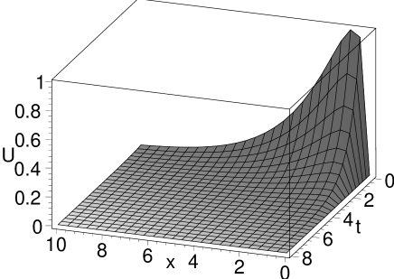
Figure 1: Exact solution (8) with $m=1,\ \lambda=3,\ \lambda_{1}=-1,\ \lambda_{2}=0,\ c_{1}=-c_{2}=4$

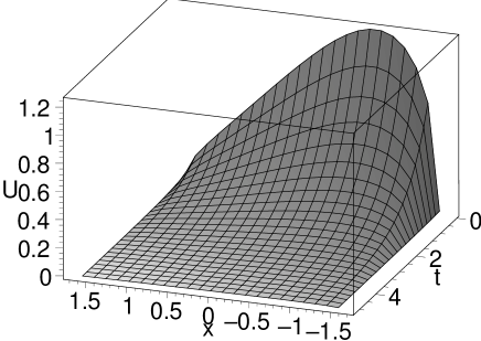
Figure 2: Exact solution (9) with $m=1,\ \lambda=2,\ \lambda_{1}=-1,\ \lambda_{2}=0,\ c_{1}=1,\ c_{2}=0$

Consider the Murray equation with the fast diffusion

$$U_{t}=\ [U^{-2}U_{x}]_{x}+\lambda U^{-2}U_{x}+\lambda_{1}U(1-U).$$ (12)

Since $\delta=\lambda^{2}>0$ solution (8) takes the form

$$U=\left[1+\exp(-\lambda_{1}t)\left(c_{1}+c_{2}\exp(-\lambda x)\right)\right]^{-1},$$ (13)

which possesses attractive properties. Assuming $c_{1}>0$ and $c_{2}>0$, one sees that this solution is positive and bounded for arbitrary $(t,x)\in\mathbb{R^{+}}\times\mathbb{R}$. Moreover solution tends either to zero ($\lambda_{1}<0$) or to 1 ($\lambda_{1}>0$) if $t\to\infty$. Both values, $U=0$ and $U=1$ are steady-state points of (12). Solution (13) tends to the steady-state point $U=0$ if $\lambda x\to-\infty$, while $U=[1+c_{1}\exp(-\lambda_{1}t)]^{-1}$ if $\lambda x\to\infty$. An example of solution (13) is presented on Fig.3 It should be also noted that (13) with $c_{1}=0$ is a travelling wave solution with the same structure as one for the Murray equation (see formula (90) in [6]).

Consider the case $(ii)$ of Theorem 1 [1]. Equation

$$\ \ \ U_{t}=\ [U^{-1}U_{x}]_{x}+\lambda U^{-1}U_{x}+(\lambda_{1}\ln U+\lambda_{2})(U-\lambda_{3}),\ \lambda_{1}\not=0,$$ (14)

and operator

$${Q}=\ \partial_{t}\ +(\lambda_{1}\ln U+\lambda_{2})U\partial_{U},$$

are transformed by the substitution (1) to the forms

$$V_{xx}=e^{V}V_{t}-\lambda V_{x}+(\lambda_{1}V+\lambda_{2})(\lambda_{3}-e^{V}),$$ (15)

and

$$Q=\partial_{t}+(\lambda_{1}V+\lambda_{2})\partial_{V},$$ (16)

respectively. Using operator (16) we obtain the ansatz

$$V=\cases{\lambda_{2}t+\varphi(x),\ \quad\lambda_{1}=0,\cr\varphi(x)e^{\lambda_{1}t}-{\lambda_{2}\over\lambda_{1}},\,\lambda_{1}\neq 0,}$$ (17)

which has the same structure as (5). Substituting (17) into (15), one again obtains integrable second-order ODEs and easily constructs the relevant exact solutions of the RDC equation (14). In the case $\lambda_{1}=0$, the solution is

$$U=\exp\left[\lambda_{2}t+c_{1}+c_{2}e^{-\lambda x}+{\lambda_{2}\lambda_{3}\over\lambda}x\right],$$ (18)

while the case $\lambda_{1}\not=0$ produces three solutions depending on $\delta=\lambda^{2}+4\lambda_{1}\lambda_{3}$:

$$U=\exp\left[\exp\left(\lambda_{1}t-{\lambda\over 2}x\right)\left(c_{1}\exp\biggr{(}\frac{\sqrt{\delta}}{2}x\biggr{)}+c_{2}\exp\biggr{(}\frac{-\sqrt{\delta}}{2}x\biggr{)}\right)-{\lambda_{2}\over\lambda_{1}}\right],\,\delta>0,$$ (19)

$$U=\exp\left[\exp\left(-\frac{\lambda}{2}x+\lambda_{1}t\right)(c_{1}+c_{2}x)-{\lambda_{2}\over\lambda_{1}}\right],\,\delta=0$$

and

$$U=\exp\left[\exp\left(-\frac{\lambda}{2}x+\lambda_{1}t\right)\left(c_{1}\cos\frac{\sqrt{-\delta}}{2}x+c_{2}\sin\frac{\sqrt{-\delta}}{2}x\right)-{\lambda_{2}\over\lambda_{1}}\right],\,\delta<0.$$ (20)

Note that properties of solutions (18)-(20) depend essentially on values of $c_{1}$ and $c_{2}$. For example, solution (19) with negative $c_{1}$ and $c_{2}$ tends to zero if $x\to\pm\infty$, while this solution infinitely increases if those constants are positive. An example of solution (19) is presented on Fig.4.

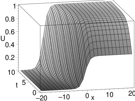
Figure 3: Exact solution (13) with $\lambda=1,\ \lambda_{1}=1,\ c_{1}=1,\ c_{2}=1$

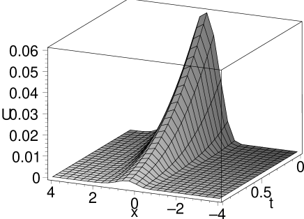
Figure 4: Exact solution (19) with $\lambda=1,\ \lambda_{1}=1,\ \lambda_{2}=1,\ \lambda_{3}=1,\ c_{1}=-1,\ c_{2}=-1$

Consider the case $(iii)$ of Theorem 1 [1]. Since we were unable to solve the overdetermined system

$$\begin{array}[]{l}\vskip 6.0pt plus 2.0pt minus 2.0pt2ff_{x}+f_{t}+fg=0,\\ \vskip 6.0pt plus 2.0pt minus 2.0ptf_{xx}-\lambda f_{x}-2g_{x}-fh=0,\\ \vskip 6.0pt plus 2.0pt minus 2.0pt(g-\frac{\lambda_{1}}{2})(g+2f_{x})+g_{t}=0,\\ \vskip 6.0pt plus 2.0pt minus 2.0pt2gh-\lambda_{1}h+2f_{x}h-\lambda_{2}f_{x}+h_{t}-\lambda g_{x}-g_{xx}=0,\\ \vskip 6.0pt plus 2.0pt minus 2.0pth^{2}-\frac{\lambda_{2}}{2}h-\lambda_{3}f_{x}+\frac{\lambda_{3}}{2}g-\lambda h_{x}-h_{xx}=0,\end{array}$$

we used the particular solution producing the $Q$-conditional operator

$${Q}=\ \partial_{t}\ +2h(x)U^{\frac{1}{2}}\partial_{U}.$$

Application of this operator leads to a solution in the implicit form

$$U=(h(x)t+\varphi(x))^{2}$$ (21)

to the nonlinear RDC equation

$$U_{t}=\ [U^{-\frac{1}{2}}U_{x}]_{x}+\lambda U^{-\frac{1}{2}}U_{x}+\lambda_{2}U^{\frac{1}{2}}\ +\lambda_{3}.$$

The functions $h$ and $\varphi$ arising in (21) satisfy the ODE system

$$\begin{array}[]{l}\vskip 6.0pt plus 2.0pt minus 2.0pth_{xx}+\lambda h_{x}-h^{2}+\frac{\lambda_{2}}{2}h=0,\\ \varphi_{xx}+\lambda\varphi_{x}-h\varphi+\frac{\lambda_{2}}{2}\varphi+\frac{\lambda_{3}}{2}=0,\end{array}$$

which is not integrable. Moreover, there are no any particular solutions of this system in the known books [7, 8]. The trivial solution of the first equation $h=\frac{\lambda_{2}}{2}$ leads to a particular case of solution (6).

Thus, we have constructed all possible exact solutions, which can be obtained by application of the $Q$-conditional symmetry operators arising in Theorem 1 [1].

Now we apply the operators arising in Theorem 2 [1] to construct exact solutions. First of all we note that the cases $(i)$ and $(ii)$ only should be considered because for cases $(iv)$ and $(v)$ the relevant work has been done in the recent paper [6]. The case $(iii)$, of course, cannot produce any new results because the Burgers equation is linearizable by the Cole-Hopf substitution.

Consider the case $(i)$ of Theorem 2 [1]. The operator

$${Q}=\ \partial_{t}-\lambda U^{m+1}\partial_{x}+(\lambda_{1}U+\lambda_{2}U^{-m})\partial_{U},$$

arising in this case can be successfully applied to construct exact solutions in the explicit form. Omitting rather trivial computations we present the final result: equation

$$U_{t}=\ [U^{m}U_{x}]_{x}+\lambda U^{m+1}U_{x}+\lambda_{2}U^{-m},\ m\neq-1;$$

possesses the solution

$$U=\left[{1\over{\lambda t+c_{1}}}\biggr{(}-x+\lambda_{2}(m+1)\left(\lambda\frac{t^{2}}{2}+c_{1}t\right)+c_{2}\biggl{)}\right]^{1\over{m+1}},$$

while

$$U=\left[{1\over{1+c_{1}e^{-\lambda_{1}(m+1)t}}}\left((m+1)\left(-{\lambda_{1}\over\lambda}x+\lambda_{2}t-{c_{1}\lambda_{2}\over\lambda_{1}(m+1)}e^{-\lambda_{1}(m+1)t}\right)+c_{2}\right)\right]^{1\over{m+1}},$$

is the exact solution of the nonlinear RDC

$$U_{t}=\ [U^{m}U_{x}]_{x}+\lambda U^{m+1}U_{x}+\lambda_{1}U+\lambda_{2}U^{-m},$$

with $\ m\neq-1,\ \lambda_{1}\neq 0$.

The most cumbersome structure of the conditional symmetry operator occurs in case $(ii)$ of Theorem 2 [1]. As consequence essential difficulties arise if one applies operator

$${Q}=\ \partial_{t}+\left(-\lambda U^{1\over 2}+{3\lambda_{1}\over 2\lambda}\right)\partial_{x}+(\lambda_{1}U^{3\over 2}+\lambda_{2}U^{1\over 2}+\lambda_{3})\partial_{U},$$ (22)

for finding exact solutions. On the other hand it will be shown that many of the exact solutions obtained possess nice properties.

Equation

$$U_{t}=\ [U^{-{1\over{2}}}U_{x}]_{x}+\lambda U^{1\over{2}}U_{x}+(\lambda_{1}U^{3\over 2}+\lambda_{2}U^{1\over 2}+\lambda_{3})\left({\lambda_{1}\over{2\lambda^{2}}}+U^{1\over 2}\right),$$ (23)

and operator (22) by the substitution (1) with $m=-1/2$ are transformed to the forms

$$V_{xx}=VV_{t}-\lambda V^{2}V_{x}-\frac{\lambda_{1}^{*}+3\lambda V}{3\lambda}\left({1\over 3}\lambda_{1}^{*}\lambda V^{3}+\lambda_{2}^{*}V+\lambda_{3}^{*}\right)$$ (24)

and

$$Q=\partial_{t}+(-\lambda V+\lambda_{1}^{*})\partial_{x}+\left({1\over 3}\lambda_{1}^{*}\lambda V^{3}+\lambda_{2}^{*}V+\lambda_{3}^{*}\right)\partial_{V},$$ (25)

respectively. Hereafter $\lambda_{1}^{*}=\frac{3\lambda_{1}}{2\lambda}\neq 0,\ \lambda_{2}^{*}={\lambda_{2}\over 2},\ \lambda_{3}^{*}={\lambda_{3}\over 2}$ and $V>0$ is assumed since (23) contains terms $U^{\frac{1}{2}}$ and $U^{-\frac{1}{2}}$. Instead of construction of a non-Lie ansatz using operator (25) (in this case it is a cumbersome procedure), one can use the equation $Q(V)=0$, i.e.

$$V_{t}=(\lambda V-\lambda_{1}^{*})V_{x}+{1\over 3}\lambda\lambda_{1}^{*}V^{3}+\lambda_{2}^{*}V+\lambda_{3}^{*},$$ (26)

to eliminate $V_{t}$ from (24). In fact, substituting the right-hand-side of (26) into (24), one arrives at

$$V_{xx}+\lambda_{1}^{*}VV_{x}+{1\over 9}{\lambda_{1}^{*}}^{2}V^{3}+{1\over 3\lambda}\lambda_{1}^{*}\lambda_{2}^{*}+{1\over 3\lambda}\lambda_{1}^{*}\lambda_{3}^{*}=0,$$ (27)

which is the non-linear ODE containing variable $t$ as a parameter. Equation (27) is reduced to the form

$$V_{yy}+3VV_{y}+V^{3}+{{3\lambda_{2}^{*}}\over{\lambda_{1}^{*}\lambda}}V+{{3\lambda_{3}^{*}}\over{\lambda_{1}^{*}\lambda}}=0$$ (28)

by the simple substitution

$$y={\lambda_{1}^{*}\over 3}x.$$ (29)

Equation (28) can be transformed into the linear third-order ODE

$$W_{yyy}+3pW_{y}+2qW=0,$$ (30)

where ${{\lambda_{2}^{*}}\over{\lambda_{1}^{*}\lambda}}=p$, ${{3\lambda_{3}^{*}}\over{\lambda_{1}^{*}\lambda}}=2q$, by the known substitution [7](see item (6.38))

$$V={W_{y}\over W}.$$ (31)

According to the classical theory of linear ODE one needs to solve the algebraic equation

$$k^{3}+3pk+2q=0,$$ (32)

which corresponds to (30). Hence four different subcases depending on the values of $p$ and $q$ should be separately considered.

Subcase 1. If $p=q=0$ then $k_{1}=k_{2}=k_{3}=0$. The general solution of (30) has the form $W=f+gy+hy^{2}$ and we arrive at the expression

$$V=\frac{g+2hy}{f+gy+hy^{2}},$$ (33)

giving the general solution of the non-linear ODE (28). Hereafter $f=f(t),\ g=g(t),\ h=h(t)$ are arbitrary (at the moment) smooth function and at least one of them must be non-zero. So (33) with (29) generates the general solution of (27) with $\lambda_{1}^{*}\neq 0.$ Finally, to obtain the general solution of system (24) and (26), it is sufficiently to substitute (33) with $y={\lambda_{1}^{*}\over 3}x$ into the second equation of this system. After the relevant calculations a cumbersome expression is obtained, however, one splits into separate parts for $x^{n},n=0,1,2$ and we arrive at the ODE system

$$\begin{array}[]{l}\vskip 6.0pt plus 2.0pt minus 2.0ptgh_{t}-g_{t}h={2\over 3}{\lambda_{1}^{*}}^{2}h^{2},\\ fh_{t}-f_{t}h={1\over 3}\lambda_{1}^{*}h(2\lambda h+\lambda_{1}^{*}g),\vskip 6.0pt plus 2.0pt minus 2.0pt\\ fg_{t}-f_{t}g={1\over 3}\lambda_{1}^{*}(2\lambda gh-2\lambda_{1}^{*}fh+\lambda_{1}^{*}g^{2}).\end{array}$$ (34)

System (34) has the similar structure to one from [6] (see formula (60)) and can be solved in a similar way. Substituting the general solution of (34) into (33) and using (29), we find the exact solutions

$$V=\frac{3}{-{\lambda_{1}^{*}}^{2}t+\lambda_{1}^{*}x+3c_{1}}$$ (35)

and

$$V=\frac{{2\lambda_{1}^{*}}(x-\lambda_{1}^{*}t)+3c_{1}}{{{\lambda_{1}^{*}}^{2}\over 3}(x-\lambda_{1}^{*}t)^{2}+c_{1}\lambda_{1}^{*}(x-\lambda_{1}^{*}t)-2\lambda\lambda_{1}^{*}t+c_{2}\lambda_{1}^{*}},$$ (36)

of the equation

$$V_{xx}=VV_{t}-\lambda V^{2}V_{x}-{\lambda_{1}^{*}\over 3}\lambda V^{4}-{{\lambda_{1}^{*}}^{2}\over 9}V^{3}.$$ (37)

Applying substitution (1) with $m=-1/2$ to (35)–(37) and renaming parameters, we arrive at the exact solutions

$$U=\left[\frac{1}{-{3\lambda_{1}^{2}\over{4\lambda^{2}}}t+{\lambda_{1}\over{2\lambda}}x+c_{1}}\right]^{2}$$

and

$$U=\left[\frac{2(x-3{\lambda_{1}\over{2\lambda}}t)+{2\lambda c_{1}\over\lambda_{1}}}{{\lambda_{1}\over{2\lambda}}(x-{3\lambda_{1}\over{2\lambda}}t)^{2}+c_{1}(x-{3\lambda_{1}\over{2\lambda}}t)-2\lambda t+c_{2}}\right]^{2}$$

of the nonlinear RDC equation

$$U_{t}=[U^{-{1\over 2}}U_{x}]_{x}+\lambda U^{1\over 2}U_{x}+\lambda_{1}U^{2}+\frac{\lambda_{1}^{2}}{2\lambda}U^{3\over 2}.$$

Subcase 2. If $p^{3}=-q^{2}\neq 0$ then $k_{1}=\alpha_{1}=-2\sqrt[3]{q}$ and $k_{2}=k_{3}=\alpha_{2}=\sqrt[3]{q}$. The general solution of (30) is

$$W=f\exp(\alpha_{1}y)+(g+yh)\exp(\alpha_{2}y),\quad\alpha_{1}=-2\alpha_{2}$$

so that the expression

$$V=\frac{\alpha_{1}f\exp(\alpha_{1}y)+(\alpha_{2}g+h(\alpha_{2}y+1))\exp(\alpha_{2}y)}{f\exp(\alpha_{1}y)+(g+yh)\exp(\alpha_{2}y)}$$

presents the general solution of the non-linear ODE (28). Dealing in quite similar way to the subcase 1, one easily obtains the ODE system

$$\begin{array}[]{l}\vskip 6.0pt plus 2.0pt minus 2.0ptgh_{t}-g_{t}h={{\lambda_{1}^{*}}\over 3}h^{2}(2\lambda\alpha_{2}+\lambda_{1}^{*}),\\ \vskip 6.0pt plus 2.0pt minus 2.0ptfh_{t}-f_{t}h=\lambda_{1}^{*}\alpha_{2}fh(\lambda\alpha_{2}-\lambda_{1}^{*}),\\ 3\alpha_{2}(fg_{t}-f_{t}g)+fh_{t}-f_{t}h=\lambda_{1}^{*}\alpha_{2}f\left(g({2\over 3}\lambda\alpha_{2}^{2}-3\alpha_{2}\lambda_{1}^{*}-{5\over 3})-h(\lambda\alpha_{2}+2\lambda_{1}^{*})\right)\end{array}$$ (38)

to find the unknown functions $f(t),\ g(t)$ and $h=h(t).$ It turns out system (38) has the same structure as one (67) from [6] and its general solution can be constructed. Finally, we find the exact solutions

$$U=\left[\frac{-2c_{1}\alpha_{2}\exp(\beta_{0}t-\beta_{1}x)+\alpha_{2}c_{2}}{c_{1}\exp(\beta_{0}t-\beta_{1}x)+c_{2}}\right]^{2},$$

and

$$U=\left[\frac{-2c_{1}\alpha_{2}\exp(\beta_{0}t-\beta_{1}x)+c_{2}\alpha_{2}(\beta_{2}t-\beta_{3}x+c_{3}+{1\over\alpha_{2}})}{c_{1}\exp(\beta_{0}t-\beta_{1}x)+c_{2}(\beta_{2}t-\beta_{3}x+c_{3})}\right]^{2}$$

of the nonlinear RDC equation

$$U_{t}=\ [U^{-{1\over{2}}}U_{x}]_{x}+\lambda U^{1\over{2}}U_{x}+(\lambda_{1}U^{3\over 2}-3\sqrt[3]{\lambda_{1}\lambda_{3}^{2}\over 4}U^{1\over 2}+\lambda_{3})\left({\lambda_{1}\over{2\lambda^{2}}}+U^{1\over 2}\right),$$

where $\beta_{0}={3\lambda_{1}\over 2\lambda}\alpha_{2}({3\lambda_{1}\over 2\lambda}-\lambda\alpha_{2}),\ \beta_{1}={3\lambda_{1}\over 2\lambda}\alpha_{2},\ \beta_{2}=-{\lambda_{1}\over 2\lambda}({3\lambda_{1}\over 2\lambda}+2\lambda\alpha_{2}),\ \beta_{3}=-{\lambda_{1}\over 2\lambda},\ \alpha_{2}=\sqrt[3]{\lambda_{3}\over 2\lambda_{1}}\not=0.$

Subcase 3. If $p^{3}+q^{2}<0$ then three roots of (32) are different and real. This case is the most cumbersome because the known Cardano formulae must be used. Let us set $k_{1}=\alpha_{1},$ $k_{2}=\alpha_{2}$ and $\ k_{3}=\alpha_{3},$ where $\alpha_{i},i=1,2,3$ are different real numbers, which are calculated by the Cardano formulae

$$\begin{array}[]{l}\alpha_{1}=-2\sqrt[6]{-p^{3}}\cos\left({1\over 3}\arctan\left({\sqrt{-p^{3}-q^{2}}\over q}\right)\right),\\ \alpha_{2}=2\sqrt[6]{-p^{3}}\cos\left({1\over 3}\arctan\left({\sqrt{-p^{3}-q^{2}}\over q}\right)-{\pi\over 3}\right),\\ \alpha_{3}=2\sqrt[6]{-p^{3}}\cos\left({1\over 3}\arctan\left({\sqrt{-p^{3}-q^{2}}\over q}\right)+{\pi\over 3}\right),\end{array}$$ (39)

if $q>0$, by the formulae

$$\begin{array}[]{l}\alpha_{1}=2\sqrt[6]{-p^{3}}\cos\left({1\over 3}\arctan\left({\sqrt{-p^{3}-q^{2}}\over q}\right)\right),\\ \alpha_{2}=-2\sqrt[6]{-p^{3}}\cos\left({1\over 3}\arctan\left({\sqrt{-p^{3}-q^{2}}\over q}\right)-{\pi\over 3}\right),\\ \alpha_{3}=-2\sqrt[6]{-p^{3}}\cos\left({1\over 3}\arctan\left({\sqrt{-p^{3}-q^{2}}\over q}\right)+{\pi\over 3}\right),\end{array}$$ (40)

if $q<0$ and by the formulae

$$\begin{array}[]{l}\alpha_{1}=0,\\ \alpha_{2}=\sqrt{-3p},\\ \alpha_{3}=-\sqrt{-3p},\end{array}$$ (41)

if $q=0$. The general solution of (30) is

$$W=f\exp(\alpha_{1}y)+g\exp(\alpha_{2}y)+h\exp(\alpha_{3}y),$$

and it leads to the general solution

$$V=\frac{\alpha_{1}f\exp(\alpha_{1}y)+\alpha_{2}g\exp(\alpha_{2}y)+\alpha_{3}h\exp(\alpha_{3}y)}{f\exp(\alpha_{1}y)+g\exp(\alpha_{2}y)+h\exp(\alpha_{3}y)}$$ (42)

of the non-linear ODE (28).

Substituting (42) with $y={\lambda_{1}^{*}\over 3}x$ into (26) and conducting the relevant calculations and splits we again arrive at the ODE system to find the unknown functions $f(t),\ g(t)$ and $h=h(t).$ This system has the form

$$\begin{array}[]{l}\vskip 6.0pt plus 2.0pt minus 2.0ptf_{t}g-fg_{t}=-{\lambda_{1}^{*}\over 3}fg(\lambda(\alpha_{1}^{2}-\alpha_{2}^{2})+\lambda_{2}(\alpha_{1}-\alpha_{2})),\\ \vskip 6.0pt plus 2.0pt minus 2.0ptf_{t}h-fh_{t}=-{\lambda_{1}^{*}\over 3}fh(\lambda(\alpha_{1}^{2}-\alpha_{3}^{2})+\lambda_{2}(\alpha_{1}-\alpha_{3})),\\ g_{t}h-gh_{t}=-{\lambda_{1}^{*}\over 3}gh(\lambda(\alpha_{2}^{2}-\alpha_{3}^{2})+\lambda_{2}(\alpha_{2}-\alpha_{3}))\end{array}$$ (43)

and is fully integrable [6]. Its general solution leads to the exact solution

$$U=\left[\frac{\alpha_{1}c_{1}\exp(\beta_{1}t+\gamma_{1}x)+\alpha_{2}c_{2}\exp(\beta_{2}t+\gamma_{2}x)+\alpha_{3}c_{3}\exp(\beta_{3}t+\gamma_{3}x)}{c_{1}\exp(\beta_{1}t+\gamma_{1}x)+c_{2}\exp(\beta_{2}t+\gamma_{2}x)+c_{3}\exp(\beta_{3}t+\gamma_{3}x)}\right]^{2}$$ (44)

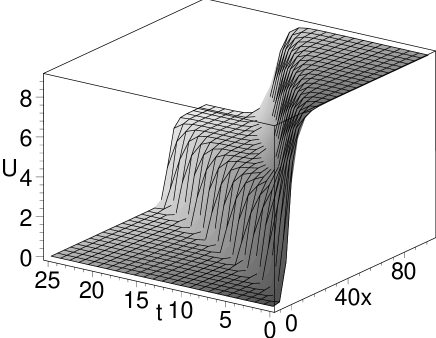
Figure 5: Exact solution (44) with $\lambda=1,\ \lambda_{1}=0.5,\ \ c_{1}=c_{2}=c_{3}=1,\ \alpha_{1}=0.1,\ \alpha_{2}=2,\ \alpha_{3}=3$

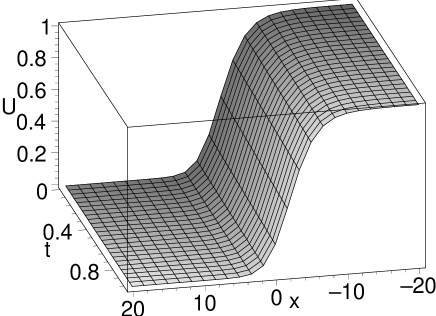
Figure 6: Exact solution (46) with $\lambda=1,\ \lambda_{2}=1,\ c_{1}=1,\ c_{2}=1,\ c_{3}=1,\ \alpha_{2}=1,\ \alpha_{3}=-1$

of the nonlinear RDC equation (23) with $\lambda_{1}\not=0$. Here $\beta_{i}=-{\lambda_{1}\over 2\lambda}(\lambda\alpha_{i}^{2}+{3\lambda_{1}\over 2\lambda}\alpha_{i}),\ \gamma_{i}={\lambda_{1}\over 2\lambda}\alpha_{i},\ i=1,2,3,$ and the roots $\alpha_{i},\ i=1,2,3$ are determined by the formulae (39)–(41) depending on the $q$ sign. In the case $c_{i}>0,i=1,2,3$, this type of exact solutions is known in applications as two-shock waves (see, e.g., [9]). An example of such solution is presented on Fig.5.

Consider the generalized FN equation with the fast diffusion

$$U_{t}=\ (U^{-\frac{1}{2}}U_{x})_{x}+\lambda U^{\frac{1}{2}}U_{x}+\lambda_{2}U^{\frac{1}{2}}(U^{\frac{1}{2}}-\delta)(1-U),\ \delta=\frac{\lambda_{2}}{2\lambda^{2}}.$$ (45)

In the case $\lambda_{2}\not=0$ and $\lambda_{3}=0$, we immediately obtain $p<0$ and $q=0$, therefore formulae (41) and (44) give the solution

$$U=\left[\frac{\alpha_{2}c_{2}\exp({\lambda_{2}\over 2\lambda}(\lambda\alpha_{2}^{2}-{3\lambda_{2}\over 2\lambda}\alpha_{2})t-{\lambda_{2}\over 2\lambda}\alpha_{2}x)+\alpha_{3}c_{3}\exp({\lambda_{2}\over 2\lambda}(\lambda\alpha_{3}^{2}-{3\lambda_{2}\over 2\lambda}\alpha_{3})t-{\lambda_{2}\over 2\lambda}\alpha_{3}x)}{c_{1}+c_{2}\exp({\lambda_{2}\over 2\lambda}(\lambda\alpha_{2}^{2}-{3\lambda_{2}\over 2\lambda}\alpha_{2})t-{\lambda_{2}\over 2\lambda}\alpha_{2}x)+c_{3}\exp({\lambda_{2}\over 2\lambda}(\lambda\alpha_{3}^{2}-{3\lambda_{2}\over 2\lambda}\alpha_{3})t-{\lambda_{2}\over 2\lambda}\alpha_{3}x)}\right]^{2}.$$ (46)

Taking into account formula (1) with $m=-1/2$, we note that solution (46) with arbitrary $c_{1},c_{2}$ and $c_{3}$ is not valid in the domain $(t,x)\in\mathbb{R^{+}}\times\mathbb{R}$. However, setting, for example, $c_{1}=0$ we obtain travelling wave solution, which is valid in this domain. An example of such solution is presented on Fig.6. It should be stressed that similar solutions possesses also the classical FN equation [10] and the generalized FN equation [6]

$$U_{t}=U_{xx}+\lambda UU_{x}+\lambda_{3}U(U-\delta)(1-U),\quad 0<\delta<1.$$

Subcase 4. If $p^{3}+q^{2}>0$ then three roots of (32) are different and two of them are complex conjugate. The Cardano formulae should be again applied. Setting $k_{1}=\alpha,$ $k_{2,3}=a\pm ib,$ where

$$\begin{array}[]{l}\alpha=\sqrt[3]{-q+\sqrt{p^{3}+q^{2}}}-\sqrt[3]{q+\sqrt{p^{3}+q^{2}}},\\ a=-{1\over 2}\left(\sqrt[3]{-q+\sqrt{p^{3}+q^{2}}}-\sqrt[3]{q+\sqrt{p^{3}+q^{2}}}\right),\\ b={\sqrt{3}\over 2}\left(\sqrt[3]{-q+\sqrt{p^{3}+q^{2}}}+\sqrt[3]{q+\sqrt{p^{3}+q^{2}}}\right),\end{array}$$ (47)

the general solution of (30) may be presented in the form

$$W=f\exp(\alpha y)+\biggr{(}g\cos(by)+h\sin(by)\biggl{)}\exp(ay),\quad\alpha=-2a.$$

Using (31) one arrives at the general solution

$$V=\frac{\alpha f\exp(\alpha y)+\biggr{(}g(a\cos(by)-b\sin(by))+h(b\cos(by)+a\sin(by))\biggl{)}\exp(ay)}{f\exp(\alpha y)+\biggr{(}g\cos(by)+h\sin(by)\biggl{)}\exp(ay)}$$

of the non-linear ODE (28). The analog of (43) in this case takes the form

$$\begin{array}[]{l}-3a(f_{t}g-fg_{t})+b(fh_{t}-f_{t}h)=bfh(\lambda_{2}^{*}-2{\lambda_{1}^{*}}^{2}a)+\\ \vskip 6.0pt plus 2.0pt minus 2.0pt+{\lambda_{1}^{*}\over 3}\lambda afg(2a^{2}+2b^{2}+5a^{3}+ab^{2}),\\ -3a(f_{t}h-fh_{t})+b(f_{t}g-fg_{t})=-bfg(\lambda_{2}^{*}-2{\lambda_{1}^{*}}^{2}a)+\\ \vskip 6.0pt plus 2.0pt minus 2.0pt{\lambda_{1}^{*}\over 3}\lambda afh(2a^{2}+2b^{2}+5a^{3}+ab^{2}),\\ gh_{t}-g_{t}h={\lambda_{1}^{*}\over 3}b(2\lambda a+\lambda_{2})(g^{2}+h^{2}).\end{array}$$ (48)

It should be stressed that the ODE system (48) has essentially different structure from those presented above and its solving takes a lot efforts. We were able to realize all necessary computations, which are omitting here, and to check the result using the program package MATHEMATICA 5.0. Finally, the exact solution

$$U=\left[\frac{-2c_{1}a\exp\left(\beta_{0}x+\beta_{1}t\right)+c_{2}\biggr{(}a\cos\left(\beta_{2}x+\beta_{3}t-c_{3}\right)-b\sin\left(\beta_{2}x+\beta_{3}t-c_{3}\right)\biggl{)}}{b_{1}\exp\left(\beta_{0}x+\beta_{1}t\right)+b_{2}\cos\left(\beta_{2}x+\beta_{3}t-c_{3}\right)}\right]^{2}$$ (49)

of the nonlinear RDC equation (23) with $\lambda_{1}\not=0$ has been found. Here $\beta_{0}=-{3\lambda_{1}\over 2\lambda}a,\ \beta_{1}=-{\lambda_{1}\over 2\lambda}(\lambda(b^{2}+3a^{2})-{9\lambda_{1}\over 2\lambda}a),\ \beta_{2}={\lambda_{1}\over 2\lambda}b,\ \beta_{3}=-{\lambda_{1}\over 2\lambda}b(2\lambda a+{3\lambda_{1}\over 2\lambda}),$ and $a$ and $b$ are determined by the formulae (47). Note that quasi-periodic periodic solutions of the similar form were also obtained for the reaction-diffusion equation

$$W_{t}=W_{yy}+\lambda WW_{y}+\lambda_{0}+\lambda_{1}W-\lambda_{3}W^{3}$$

with $\lambda=0$ [11, 12].

3. Conclusions.

In the first part of this paper [1], Theorems 1 and 2 giving a complete description of $Q$-conditional symmetries of the nonlinear RDC equations (2) – (3) are proved. It should be stressed that all $Q$-conditional symmetry operators listed in Theorems 1–2 [1] contains the same nonlinearities with respect to the dependent variable $U$ as the relevant RDC equations. Analogous results were earlier obtained for single reaction-diffusion equations [11], [13], [14], [15].

However, we note that there is the essential difference between RDC equations (2) – (3) and the relevant RD equation

$$U_{t}=[U^{m}U_{x}]_{x}+C(U).$$

For example, the Murray type equation

$$U_{t}=U_{xx}+\lambda UU_{x}+\lambda_{0}+\lambda_{2}U^{2},\quad\lambda_{2}\not=0,$$

admits the $Q$-conditional symmetry

$$\quad\quad\quad Q=\partial_{t}+\left(-\lambda U+{\lambda_{2}\over\lambda}\right)\partial_{x}+(\lambda_{0}+\lambda_{2}U^{2})\partial_{U},$$

while the RD equation with this term, i.e. the Fisher type equation

$$U_{t}=U_{xx}+\lambda_{0}+\lambda_{1}U+\lambda_{2}U^{2},\quad\lambda_{2}\not=0$$

does not possess one. Similarly, the RDC equation (23) possessing the $Q$-conditional symmetry (22) has no analog among reaction-diffusion equations with the diffusivity $U^{-{1\over 2}}$.

The RDC equations listed in Theorems 1 and 2 [1] contain several well-known equations arising in applications and their direct generalizations. In the particular case, the Murray equation, its porous analog (11) and its analog with the fast diffusion

$$U_{t}=\ [U^{-2}U_{x}]_{x}+\lambda U^{-2}U_{x}+\lambda_{1}U(1-U);$$

the Fitzhugh-Nagumo equation [16] with the convective term

$$U_{t}=U_{xx}+\lambda UU_{x}+\lambda_{3}U(U-\delta)(1-U),\quad 0<\delta<1$$

and its analog (45) with the fast diffusion; the Kolmogorov-Petrovskii-Piskunov equation [17] with the convective term

$$U_{t}=U_{xx}+\lambda UU_{x}+\lambda_{3}U(1-U)^{2},$$

and the Newell-Whitehead equation [18] with the convective term

$$U_{t}=U_{xx}+\lambda UU_{x}+\lambda_{3}U^{3}-\lambda_{1}U.$$

A further generalization of the RDC equations (2) and (3) reads as

$$U_{t}=[U^{m}U_{x}]_{x}+\lambda U^{n}U_{x}+C(U),\quad\lambda\not=0,$$ (50)

where $m$ and $n$ are arbitrary constants. The work is in progress on the complete description of $Q$-conditional symmetry of (50) and the RDC equation with exponential nonlinearities

$$U_{t}=[\exp(mU)U_{x}]_{x}+\lambda\exp(nU)U_{x}+C(U),\quad\lambda\not=0.$$

It is well-known that new $Q$-conditional symmetries don’t guarantee the construction of exact solutions, which cannot be obtained by the Lie machinery (see non-trivial examples in [2, 3]). In this paper, several exact solutions were constructed using the conditional symmetries arising in Theorem 1 and 2 [1]. It was shown that these solutions are not obtainable by Lie symmetries, however, they contain the known plane wave solutions as particular cases. Many of the solutions obtained possess attractive properties and can be used for further investigation of the relevant boundary-value problems. In the particular case, we established that the zero Dirichlet and Neumann conditions, i.e. typical boundary conditions for mathematical models arising in physics and biology, can be satisfied by the relevant fitting of constants $c_{1},\ c_{2}$ and $c_{3}$ (see the solutions presented on Fig.1-2, 4-6).

To our best knowledge many of the solutions presented above are new. However, we noted that some of them can be derived from the recent paper [19]. In fact, if one applies substitution (1) to the RDC equation (10) and its solutions (8)-(9), then equation (54)[19] with (65)-(66) [19] and $\alpha(s)=s^{n},$ and solutions (69)-(71) [19] are exactly obtained. Nevertheless the authors of that paper don’t use any symmetries to construct exact solutions, formula (72) [19] is nothing else but the equation $Q(V)=0,$ where $Q$ is the conditional symmetry operator

$$Q=\partial_{t}+(\lambda_{1}^{*}V+\lambda_{2}^{*})\partial_{V}$$

of

$$V_{xx}=V^{n}V_{t}-\lambda V_{x}+(\lambda_{1}^{*}V+\lambda_{2}^{*})(\lambda_{3}-V^{n}).$$

Thus, we obtain new confirmation of the known idea (see, i.e. [13], [20]) that any exact solution can be obtained by the relevant Lie or conditional symmetry operator.

References

[1] Cherniha R, Pliukhin O 2006 New conditional symmetries and exact solutions of nonlinear
reaction-diffusion-convection equations. I (math-ph/0612078)
[2] Cherniha R 1996
A constructive method for construction of new exact solutions of
nonlinear evolution equations. Rep. Math. Phys.38
301-312
[3] Cherniha R 1998
New Non-Lie Ansätze and Exact Solutions of Nonlinear
Reaction-Diffusion-Convection Equations J. Phys. A: Math.Gen.31 8179-8198
[4] Cherniha R, Serov M 1998
Symmetries, Ansätze and Exact Solutions of Nonlinear
Second-order Evolution Equations with Convection Term Euro. J. Appl. Math.9 527–542
[5] Cherniha R, Serov M 2006
Symmetries, Ansätze and Exact Solutions of Nonlinear
Second-order Evolution Equations with Convection Term II Euro. J. Appl. Math.17 597-605.
[6] Cherniha R 2007 New -conditional Symmetries and Exact Solutions
of Some Reaction-Diffusion-Convection Equations
Arising in Mathematical Biology J. Math. Anal. Appl.326 783–799
[7] Kamke E 1959 Differentialgleichungen.
Lösungmethoden and Lösungen (6-th Ed. Leipzig)
(in German).
[8] Polyanin A D, Zaitsev V F 2003 Handbook of
exact solutions for ordinary differential equations (CRC Press
Company)
[9] Liu Q M Fokas A S 1996
Exact interaction of solitary waves for certain nonintegrable
equations J. Math. Phys.37 324–345.
[10] Kawahara T, Tanaka M 1983
Interactions of traveling fronts: an exact solution of a nonlinear
diffusion equation
Phys. Lett. A97 311–314.
[11] Clarkson P A and Mansfield E L 1993
Symmetry reductions and exact solutions of a class of nonlinear heat
equations Physica D 70 250-288
[12] Dixon J M, Tuszynski J A, Clarkson P A 1997
From Nonlinearity to Coherence (Oxford: Clarendon Press)
[13] Fushchych W I, Shtelen W M, Serov M I 1993
Symmetry analysis and exact solutions of equations of nonlinear
mathematical physics (Dordrecht: Kluwer)
[14] Serov M I 1990
Conditional invariance and exact solutions of non-linear heat
equation Ukrainian Math. J.42 1370–76
[15] Nucci M C 1992
Symmetries of linear, -integrable, -integrable and
nonintegrable equations and dynamical systems Nonlinear
evolution equations and dynamical systems (River Edge: World Sci.
Publ. (USA)) 374-381
[16] Fitzhugh R 1961
Impulse and physiological states in models of nerve membrane Biophys. J.1 445–466
[17] Kolmogoroff A, Petrovsky I, Piskounoff N 1937
Étude de l’équation de la diffusion avec croissance de la
quantité de matière et son application à un problème
biologique Moscow Univ. Bull. Math.1 1–25 (in
French)
[18] Newell A C, Whitehead J A 1969
Finite bandwidth, finite amplitude convection J. Fluid Mech.38 279-303
[19] Carini M, Fusco D, Manganaro N 2003 Wave-Like
Solutions for a Class of Parabolic Models Nonlinear Dynamics32 211-222
[20] Bluman G W and Cole I D 1969
The general similarity solution of the heat equation
J. Math. Mech.18 1025-42