Non-perturbative embedding of local defects in crystalline materials

Abstract

We present a new variational model for computing the electronic first-order density matrix of a crystalline material in presence of a local defect. A natural way to obtain variational discretizations of this model is to expand the difference $Q$ between the density matrix of the defective crystal and the density matrix of the perfect crystal, in a basis of precomputed maximally localized Wannier functions of the reference perfect crystal. This approach can be used within any semi-empirical or Density Functional Theory framework.

Describing the electronic state of crystals with local defects is a major issue in solid-state physics, materials science and nano-electronics [1, 2, 3]. The first self-consistent electronic structure calculations for defective crystals were performed in the late 70’, by means of nonlinear Green functions methods [4, 5, 6]. In the 90’, it became possible to solve the Kohn-Sham equations [7] for systems with several hundreds of electrons, and Green function methods were superseded by supercell methods [8, 9]. However, supercell methods have several drawbacks. First, the defect interacts with its periodic images. Second, the supercell must have a neutral total charge, so that in the simulation of charged defects, an artificial charge distribution (a jellium for instance) needs to be introduced to counterbalance the charge of the defect. These two drawbacks may lead to large, uncontrolled errors in the estimation of the energy of the defect. In practice, ad hoc correction terms are introduced to account for these errors [10]. A refinement of the supercell approach, based on a more careful treatment of the Coulomb interaction, has also been proposed in [11].

In a recent article [12], we have used rigorous thermodynamic limit arguments to derive a variational model allowing to directly compute the modification of the electronic first order density matrix generated by a (neutral or charged) local defect, when the host crystal is an insulator (or a semi-conductor). This model has a structure similar to the Chaix-Iracane model in quantum electrodynamics [13, 14]. This similarity originates from formal analogies between the Fermi sea of a defective crystal and the Dirac sea in presence of atomic nuclei. For technical reasons, the reference model considered in [12] was the reduced Hartree-Fock model, or in other words, a Kohn-Sham model with fractional occupancies and exchange-correlation energy set to zero.

The purpose of the present article is twofold. First, the extension of our model to a generic exchange-correlation functional is discussed. Second, a rigorous justification of the numerical method consisting in expanding the difference between the density matrix of the defective crystal and the density matrix of the perfect crystal, in a basis of well-chosen Wannier functions of the reference perfect crystal, is provided: this method can be seen as a variational approximation of our model.

1 Derivation of the model

We consider a generic Kohn-Sham model (or rather a generic extended Kohn-Sham model in which fractional occupancies are allowed) with exchange correlation energy functional $E^{\rm xc}(\rho)$. For the sake of simplicity, we omit the spin variable. The ground state of a molecular system with nuclear charge density $\rho^{\rm nuc}$ and ${\mathcal{N}}$ electrons is obtained by solving

$$\inf\left\{E^{\rm KS}_{\rho^{\rm nuc}}(\gamma),\;0\leq\gamma\leq 1,\;\Tr(\gamma)={\mathcal{N}}\right\},$$ (1)

$$E^{\rm KS}_{\rho^{\rm nuc}}(\gamma)=\Tr\left(-\frac{1}{2}\Delta\gamma\right)-D(\rho^{\rm nuc},\rho_{\gamma})+\frac{1}{2}D(\rho_{\gamma},\rho_{\gamma})+E^{\rm xc}(\rho_{\gamma}),$$ (2)

where $\rho_{\gamma}(\mathbb{r})=\gamma(\mathbb{r},\mathbb{r})$ and where

$$D(f,g)=\int_{\mathbb{R}^{3}}\int_{\mathbb{R}^{3}}\frac{f(\mathbb{r})\,g(\mathbb{r}^{\prime})}{|\mathbb{r}-\mathbb{r}^{\prime}|}\,d\mathbb{r}\,d\mathbb{r}^{\prime}$$

is the Coulomb interaction. Still for simplicity, we detail the case of the X$\alpha$ exchange-correlation functional

$$E^{\rm xc}(\rho)=-C_{{\rm X}\alpha}\int_{\mathbb{R}^{3}}\rho^{4/3},$$

the extension to more accurate LDA functionals being straightforward. Likewise, replacing the all electron model considered here with a valence electron model with pseudopotentials does not bring any additional difficulty.

The above model describes a finite system of $\mathcal{N}$ electrons in the electrostatic field created by the density $\rho^{\rm nuc}$. Our goal is to describe an infinite crystalline material obtained in the thermodynamic limit $\mathcal{N}\to\infty$. In fact we shall consider two such systems. The first one is the periodic crystal obtained when, in the thermodynamic limit, the nuclear density approaches the periodic nuclear distribution of the perfect crystal:

$$\rho^{\rm nuc}\rightarrow\rho_{\rm per}^{\rm nuc},$$ (3)

$\rho^{\rm nuc}_{\rm per}$ being a periodic distribution. The second system is the previous crystal in presence of a local defect:

$$\rho^{\rm nuc}\rightarrow\rho_{\rm per}^{\rm nuc}+\nu.$$ (4)

Typically, $\nu$ describes nuclear vacancies, interstitial nuclei, or impurities together with possible local rearrangement of the nuclei of the host crystal in the vicinity of the defect. In the simple case of a reference perfect crystal with a single atom per unit cell

$$\rho^{\rm nuc}_{\rm per}=\sum_{\mathbb{R}\in{\cal R}}z\delta_{\mathbb{R}}$$

where $\cal R$ is the Bravais lattice of the host crystal and $\delta_{\mathbb{R}}$ is the Dirac delta measure at $\mathbb{R}$. If the defect consists in a impurity (the nucleus of charge $z$ at $\mathbb{R}={\mathbb{0}}$ being replaced with a nucleus of charge $z^{\prime}$), the charge distribution $\nu$ reads

$$\nu=z^{\prime}\delta_{\mathbb{U}({\mathbb{0}})}-z\delta_{\mathbb{0}}+\sum_{\mathbb{R}\in{\cal R}\setminus\left\{0\right\}}z\left(\delta_{\mathbb{R}+\mathbb{U}(\mathbb{R})}-\delta_{\mathbb{R}}\right),$$

where $\mathbb{U}$ is the displacement field of the nuclei generated by the relaxation of the crystal. It is therefore composed of nuclei of positive charges and of “ghost nuclei” of negative charges. In this article, we assume that $\nu$ is given, and we focus on the calculation of the electronic density matrix.

The form of the density matrix $\gamma^{0}_{\rm per}$ of the perfect crystal obtained in the thermodynamic limit (3) is well-known. The matrix $\gamma^{0}_{\rm per}$ is a solution to the self-consistent equation

$$\gamma^{0}_{\rm per}=\chi_{(-\infty;\epsilon_{F}]}(H^{0}_{\rm per})$$ (5)

$$H^{0}_{\rm per}=-\frac{1}{2}\Delta+\Phi_{\rm per}-\frac{4}{3}C_{{\rm X}\alpha}\,{\rho^{0}_{\rm per}}^{\!\!\!\!\!1/3},$$ (6)

$$-\Delta\Phi_{\rm per}=4\pi\left(\rho_{\rm per}^{0}-\rho_{\rm per}^{\rm nuc}\right),\quad\Phi_{\rm per}\mbox{ ${\mathcal{R}}$-periodic}.$$

The notation $P=\chi_{(-\infty;\epsilon_{\rm F}]}(A)$ means that $P$ is the spectral orthogonal projector of the self-adjoint operator $A$ corresponding to filling all the energies up to the Fermi level $\epsilon_{\rm F}$ (see for instance [15]). In our case, (5) means that $\gamma^{0}_{\rm per}$ is the spectral projector which fills all the energies of $H^{0}_{\rm per}$ up to the Fermi level $\epsilon_{\rm F}$, see Figure 1.

Figure 1: Spectrum of $H^{0}_{\rm per}$.

The density of the periodic Fermi sea is $\rho^{0}_{\rm per}(\mathbb{r})=\gamma^{0}_{\rm per}(\mathbb{r},\mathbb{r})$. Note that the system is locally neutral:

$$\int_{\Omega}\rho^{0}_{\rm per}=\int_{\Omega}\rho^{\rm nuc}_{\rm per},$$

where $\Omega$ is a reference unit cell, the Fermi level $\epsilon_{\rm F}$ being chosen to ensure this equality. For the rest of the article, we assume that the host crystal is an insulator (or a semi-conductor), i.e. that there is a gap $g=\Sigma^{+}-\Sigma^{-}>0$ between the highest occupied and the lowest virtual bands. Then the Fermi level can be any number $\Sigma^{-}\leq\epsilon_{\rm F}<\Sigma^{+}$.

Now we consider the system obtained in the thermodynamic limit (4) when there is a defect $\nu$ and derive a nonlinear variational model for it. We shall describe the variations of the Fermi sea with respect to the periodic state $\gamma^{0}_{\rm per}$. The relevent variable therefore is

$$Q=\gamma-\gamma^{0}_{\rm per}$$

where $\gamma$ is the density matrix of the defective Fermi sea. Notice that the constraint that $\gamma$ is a density matrix ($0\leq\gamma\leq 1$) translates into $-\gamma^{0}_{\rm per}\leq Q\leq 1-\gamma^{0}_{\rm per}$ for the new variable $Q$.

The energy of $Q$ is by definition the difference of two infinite quantities: the energy of the state $\gamma$ and the energy of the periodic Fermi sea $\gamma^{0}_{\rm per}$. Using (2), one obtains:

$$\mathcal{E}^{\nu}(Q)=\Tr(H^{0}_{\rm per}Q)-D(\nu,\rho_{Q})+\frac{1}{2}D(\rho_{Q},\rho_{Q})+\epsilon^{\rm xc}(\rho_{Q})$$ (7)

where

$$\epsilon^{\rm xc}(\rho_{Q})=-C_{{\rm X}\alpha}\int_{\mathbb{R}^{3}}(\rho^{0}_{\rm per}+\rho_{Q})^{4/3}-{\rho^{0}_{\rm per}}^{\!\!\!\!\!4/3}-\frac{4}{3}{\rho^{0}_{\rm per}}^{\!\!\!\!\!1/3}\rho_{Q}.$$

If we want to describe a defective crystal of electronic charge $q$ ($q$ electrons in excess with respect to the perfect crystal if $q>0$, or $-q$ holes if $q<0$) interacting with the self-consistent Fermi sea in the presence of the defect, we have to consider the minimization principle

$$E^{\nu}(q)=\inf\left\{\mathcal{E}^{\nu}(Q),\,-\gamma^{0}_{\rm per}\leq Q\leq 1-\gamma^{0}_{\rm per},\;\Tr(Q)=q\right\}.$$ (8)

We obtain in this way a model which apparently renders possible the direct calculation of the defective Fermi sea in presence of the nuclear charge defect $\nu$, when $q$ electrons (or $-q$ holes) are trapped by the defect. A globally neutral system would correspond to $q=\int_{\mathbb{R}^{3}}\nu$ but there is no obstacle in applying (8) to charged defects.

Alternatively, one can, instead of imposing a priori the total charge $q$ of the system (microcanonical viewpoint), rather fix the Fermi level $\epsilon_{\rm F}\in(\Sigma^{-},\Sigma^{+})$ (grand-canonical viewpoint). This amounts to considering the Legendre transform of (8):

$$E^{\nu}_{\epsilon_{\rm F}}=\inf\left\{\mathcal{E}^{\nu}(Q)-\epsilon_{\rm F}\Tr(Q),\,-\gamma^{0}_{\rm per}\leq Q\leq 1-\gamma^{0}_{\rm per}\right\}.$$ (9)

Any solution of (8) or (9) satisfies the SCF equation

$$Q=\chi_{(-\infty,\epsilon_{\rm F})}\left(H_{Q}\right)-\gamma^{0}_{\rm per}+\delta,$$ (10)

where

$$H_{Q}=-\frac{\Delta}{2}+\Phi_{\rm per}+(\rho_{Q}-\nu)\ast\frac{1}{|x|}-\frac{4}{3}C_{{\rm X}\alpha}(\rho^{0}_{\rm per}+\rho_{Q})^{1/3}$$

and where $0\leq\delta\leq 1$ is a finite-rank self-adjoint operator on $L^{2}(\mathbb{R}^{3})$ such that $\mbox{Ran}(\delta)\subset\mbox{Ker}(H_{Q}-\epsilon_{\rm F})$. In the case of (8), the Fermi level $\epsilon_{\rm F}$ is the Lagrange multiplier associated with the constraint $\Tr(Q)=q$. The essential spectrum of $H_{Q}$ is the same as the one of $H^{0}_{\rm per}$ and is therefore composed of bands. On the other hand, the discrete spectrum of $H^{0}_{\rm per}$ is empty, while the discrete spectrum of $H_{Q}$ may contain isolated eigenvalues of finite multiplicities located below the essential spectrum and between the bands. Each filled (or unfilled) eigenvalue may correspond to electrons (or holes) which are trapped by the defect.

Figure 2: Spectrum of $H_{Q}$.

The SCF equation (10) is equivalent to the usual Dyson equation, which is at the basis of Green function methods.

2 Proper definition of the variational set

The variational models (8) and (9) may look similar to the usual Kohn-Sham models for molecules and perfect crystals. Their mathematical structure is however dramatically more complex. To design consistent numerical methods for solving (8) and (9), a deeper understanding of the mathematical setting is needed.

The biggest issue with problems (8) and (9) is to properly define the variational set, that is the set of all $Q$’s on which one has to minimize the energy functional ${\mathcal{E}}^{\nu}(Q)$ or the free energy functional ${\mathcal{E}}^{\nu}(Q)-\epsilon_{\rm F}\Tr(Q)$. For usual Kohn-Sham models, the variational set is very simple: it is the largest set of density matrices for which each term of the energy functional is a well-defined number and the constraints are satisfied. This is the reason why it is not a problem to omit the precise definition of the variational set when dealing with usual Kohn-Sham models. For instance, the variational set for (1) is

$$\left\{\gamma\;|\;0\leq\gamma\leq 1,\;\Tr(\gamma)={\mathcal{N}},\;\Tr(|\nabla|\gamma|\nabla|)<\infty\right\}.$$ (11)

Let us recall (see [15] for instance) that if $B$ is a non-negative self-adjoint operator on $L^{2}(\mathbb{R}^{3})$ and if $(\psi_{i})_{i\in\mathbb{N}}$ is an orthonormal basis of $L^{2}(\mathbb{R}^{3})$, the series of non-negative numbers $\sum_{i=0}^{+\infty}\langle\psi_{i}|B|\psi_{i}\rangle$ converges in $\mathbb{R}_{+}\cup\left\{+\infty\right\}$ towards a limit denoted by $\Tr(B)$, which does not depend on the chosen basis. The operator $B$ is said to be trace-class if $\Tr(B)<\infty$. A bounded operator $A$ on $L^{2}(\mathbb{R}^{3})$ is trace-class if $\sqrt{A^{\ast}A}$ is trace-class. In this case, the scalar $\Tr(A)=\sum_{i=0}^{+\infty}\langle\psi_{i}|A|\psi_{i}\rangle$ is well-defined and does not depend on the chosen basis. On the other hand, if $A$ is not trace-class, the series $\sum_{i=0}^{+\infty}\langle\psi_{i}|A|\psi_{i}\rangle$ may converge for one specific basis and diverge (or converge to a different limit) in another basis.

The condition $\Tr(|\nabla|\gamma|\nabla|)<\infty$ in (11) is a necessary and sufficient condition for each term of (2) being well-defined. In terms of Kohn-Sham orbitals, this conditions means that each orbital $\phi_{i}$ is in the Sobolev space $H^{1}(\mathbb{R}^{3})=\left\{\phi\in L^{2}(\mathbb{R}^{3})\;|\;\nabla\phi\in(L^{2}(\mathbb{R}^{3}))^{3}\right\}$.

The difficulty with the variational models (8) and (9) is that the variational set has not so simple a structure. It was shown in [12] that an appropriate variational set is the convex set

$${\mathcal{K}}=\big{\{}Q\ |\ -\gamma^{0}_{\rm per}\leq Q\leq 1-\gamma^{0}_{\rm per},\ \Tr(1+|\nabla|)Q^{2}(1+|\nabla|)\\ +\Tr(1+|\nabla|)(Q^{++}-Q^{--})(1+|\nabla|)<\infty\big{\}}.$$

In the above expression, we have used the notation

$$Q=\quad\left(\begin{array}[]{c||c}Q^{--}&Q^{-+}\\ \hline\cr\hline\cr Q^{+-}&Q^{++}\\ \end{array}\right)$$

with

$$Q^{--}=\gamma^{0}_{\rm per}Q\gamma^{0}_{\rm per},\;\;Q^{-+}=\gamma^{0}_{\rm per}Q(1-\gamma^{0}_{\rm per}),$$

$$Q^{+-}=(1-\gamma^{0}_{\rm per})Q\gamma^{0}_{\rm per},\;\;Q^{++}=(1-\gamma^{0}_{\rm per})Q(1-\gamma^{0}_{\rm per}),$$

corresponding to the decomposition

$$L^{2}(\mathbb{R}^{3})={\cal H}_{-}\oplus{\cal H}_{+},$$ (12)

where ${\mathcal{H}}_{-}=\gamma^{0}_{\rm per}L^{2}(\mathbb{R}^{3})$ and ${\mathcal{H}}_{+}=(1-\gamma^{0}_{\rm per})L^{2}(\mathbb{R}^{3})$ are respectively the occupied and virtual spaces of the reference perfect crystal.

Notice that when $Q$ satisfies the constraint $-\gamma^{0}_{\rm per}\leq Q\leq 1-\gamma^{0}_{\rm per}$, one has $Q^{++}\geq 0$ and $Q^{--}\leq 0$. A remarkable point, proved in [12], is that the density $\rho_{Q}$ of any operator $Q\in\mathcal{K}$ is a well-defined function which satisfies

$$\int_{\mathbb{R}^{3}}\rho_{Q}^{2}+D(\rho_{Q},\rho_{Q})<\infty.$$

This shows that the electrostatic components of the energy ${\mathcal{E}}^{\nu}(\gamma)$ are well-defined and that so is the exchange-correlation contribution: as $\rho^{0}_{\rm per}$ is periodic, continuous and positive on $\mathbb{R}^{3}$ and as $\rho_{Q}\in L^{2}(\mathbb{R}^{3})$, the fifth term of (7) which was not considered in [12] is also well-defined. Finally, following [16], the generalized trace of an operator $Q\in\mathcal{K}$ is defined by

$$\Tr(Q)=\Tr(Q^{++})+\Tr(Q^{--}),$$ (13)

and for any $Q\in\mathcal{K}$, one sets

$$\Tr(H^{0}_{\rm per}Q)=\Tr([H^{0}_{\rm per}]^{++}Q^{++})+\Tr([H^{0}_{\rm per}]^{--}Q^{--}),$$

where $[H^{0}_{\rm per}]^{--}$ and $[H^{0}_{\rm per}]^{++}$ are respectively the restrictions to the occupied and virtual spaces of the periodic Kohn-Sham hamiltonian of the perfect crystal. Note that $H^{0}_{\rm per}$ is block diagonal in the decomposition (12):

$$H^{0}_{\rm per}=\quad\left(\begin{array}[]{c||c}[H^{0}_{\rm per}]^{--}&0\\ \hline\cr\hline\cr 0&[H^{0}_{\rm per}]^{++}\\ \end{array}\right).$$

The definition (13) of the trace function is an extension of the standard trace function defined on the set of trace-class operators. Note that this extension depends of $\gamma^{0}_{\rm per}$ through the decomposition (12) of the $L^{2}$ space. In the Quantum Electrodynamical model studied in [16, 17, 18, 14, 19], minimizers are never trace-class (this property being related to renormalization). Whether or not the minimizers of  (8) and (9) are trace-class still is an open question.

To our knowledge, the variational interpretation of the ground state solutions of the self-consistent equation (10) as minimizers of the energy (7) on the set ${\cal K}$ with a constraint on the generalized trace (13), is new. This interpretation allows to rigorously justify the numerical method described in Section 4.

3 Interpretation in terms of Bogoliubov states

The density matrix formalism used in the previous section can be reinterpreted in terms of Bogoliubov states, following [13].

Let $\gamma$ be an orthogonal projector acting on $L^{2}(\mathbb{R}^{3})$ such that $Q=\gamma-\gamma^{0}_{\rm per}\in{\mathcal{K}}$. It can be proved [18] that there exists an orthonormal basis $(\phi_{i}^{-})_{i\geq-N_{-}}$ of ${\cal H}_{-}$ and an orthonormal basis $(\phi_{i}^{+})_{i\geq-N_{+}}$ of ${\cal H}_{+}$ such that in this basis

$$Q=\quad\left(\begin{array}[]{c|c||c|c}-I_{N_{-}}&0&0&0\\ \hline\cr 0&\mbox{diag}(-p_{i})&0&\mbox{diag}(p_{i}^{\prime})\\ \hline\cr\hline\cr 0&0&I_{N_{+}}&0\\ \hline\cr 0&\mbox{diag}(p_{i}^{\prime})&0&\mbox{diag}(p_{i})\\ \end{array}\right)$$ (14)

with $0\leq p_{i}<1$, $\sum_{i=0}^{+\infty}p_{i}<\infty$, $p_{i}^{\prime}=\sqrt{p_{i}(1-p_{i})}$. Notice that $Q$ is a trace-class operator if and only if $\sum_{i=0}^{+\infty}\sqrt{p_{i}}<\infty$. Let us assume for simplicity that in equation (10), the Fermi level $\epsilon_{\rm F}$ is either empty or fully occupied. In this case, $\chi_{(-\infty,\epsilon_{\rm F})}\left(H_{Q}\right)+\delta$ is an orthogonal projector, which implies that $Q$ can be decomposed as in (14). It is important to mention that in this case, the generalized trace of $Q$ is the integer $N_{+}-N_{-}$.

Formula (14) can be interpreted in terms of Bogoliubov states. The orbitals $\phi_{-N_{+}}^{+},\cdots,\phi_{-1}^{+}$ describe bound electrons in the virtual bands of the reference perfect crystal, while the orbitals $\phi_{-N_{-}}^{-},\cdots,\phi_{-1}^{-}$ represent bound holes in the occupied bands. Likewise, each pair $(\phi_{i}^{+},\phi_{i}^{-})$ with $i\geq 0$ and $0<p_{i}<1$ is a virtual electron-hole pair, and $\phi_{i}^{+}$ and $\phi_{i}^{-}$ are the states of the corresponding Bogoliubov quasiparticles. The angle $\theta_{i}=\mbox{asin}(p_{i})$ is then called the Bogoliubov angle of the virtual pair.

Formula (14) can itself be rewritten in a second quantized form, using the Fock space built upon the decomposition (12). Let us introduce the $N$-electron sector $\mathcal{F}_{+}^{N}:=\bigwedge_{1}^{N}\mathcal{H}_{+}$ and the $M$-hole sector $\mathcal{F}_{-}^{M}:=\bigwedge_{1}^{M}\mathcal{H}_{-}$. The electron-hole Fock space is defined as

$$\mathcal{F}:=\bigoplus_{N,M\geq 0}\mathcal{F}_{+}^{N}\otimes\mathcal{F}_{-}^{M}.$$

We denote by $a_{i}^{\dagger}$ the creation operator of an electron in the state $\phi^{+}_{i}$ and by $b_{i}^{\dagger}$ the creation operator of a hole in the state $\phi^{-}_{i}$. In this formalism, the vacuum state $\Omega_{0}=1\otimes 1\in\mathcal{F}_{+}^{0}\otimes\mathcal{F}^{0}_{-}$ corresponds to the periodic Fermi sea of the perfect crystal, represented by the density matrix $\gamma^{0}_{\rm per}$ in the usual Kohn-Sham description. We may also define the charge operator acting on the Fock space $\mathcal{F}$ by

$${\cal Q}=\sum_{i\geq-N_{+}}a_{i}^{\dagger}a_{i}-\sum_{i\geq-N_{-}}b_{i}^{\dagger}b_{i}.$$

There is a special subclass of states in $\mathcal{F}$ called Bogoliubov states [13, 16, 20, 21]. Each Bogoliubov state $\Omega_{\gamma}\in\mathcal{F}$ is completely characterized by its one-body density matrix $\gamma$, an orthogonal projector acting on $L^{2}(\mathbb{R}^{3})$. Conversely, any projector $\gamma$ gives rise to a Bogoliubov state under the Shale-Stinespring [22, 23] condition that $Q=\gamma-\gamma^{0}_{\rm per}$ is a Hilbert-Schmidt operator (which means $\Tr(Q^{2})<\infty$). The role of the Shale-Stinespring condition is to ensure that $\Omega_{\gamma}$ is a well-defined state in the same Fock space as the vacuum state $\Omega_{0}$. Saying differently, this ensures that the Fock space representation associated with the splitting $L^{2}(\mathbb{R}^{3})=\gamma L^{2}(\mathbb{R}^{3})\oplus(1-\gamma)L^{2}(\mathbb{R}^{3})$ is equivalent to the one induced by (12) (i.e. $L^{2}(\mathbb{R}^{3})=\gamma^{0}_{\rm per}L^{2}(\mathbb{R}^{3})\oplus(1-\gamma^{0}_{\rm per})L^{2}(\mathbb{R}^{3})$). Notice the Hilbert-Schmidt condition $\Tr(Q^{2})<\infty$ is satisfied for any $Q=\gamma-\gamma^{0}_{\rm per}$ in $\mathcal{K}$. Hence the variational set $\cal K$ can be identified with a variational set of Bogoliubov states $\{\Omega_{\gamma}\}_{\gamma\in\cal K}$ in the Fock space $\cal F$.

The expression of the Bogoliubov state $\Omega_{\gamma}$ in the Fock space $\mathcal{F}$ is given by [21, 22, 24]

$$\Omega_{\gamma}=c\;a^{\dagger}_{-N_{+}}\cdots a^{\dagger}_{-1}b^{\dagger}_{-N_{-}}\cdots b^{\dagger}_{-1}\exp\left(\sum_{i\geq 0}\lambda_{i}a^{\dagger}_{i}b^{\dagger}_{i}\right)\Omega_{0}$$

where $\lambda_{i}=\tan(\theta_{i})$, and where $c$ is a normalization constant. The above expression can be considered as the second-quantized formulation of (14). It can then easily be checked [16] that the charge of each Bogoliubov state $\Omega_{\gamma}$ (counted relatively to that of the vacuum $\Omega_{0}$) is actually given by (13):

$${\langle\Omega_{\gamma}|{\cal Q}|\Omega_{\gamma}\rangle}=\Tr(Q^{++})+\Tr(Q^{--})=N_{+}-N_{-}$$

where $Q=\gamma-\gamma^{0}_{\rm per}$.

4 Variational approximation

Let us now come to the discretization of problem (8).

If one discretizes (8) in a local basis without taking care of the constraint $Q\in{\cal K}$, there is a risk to obtain meaningless numerical results. On the other hand, selecting a basis set which respects the decomposition (12), will lead to a well-behaved variational approximation of (8) (the constraint $Q\in{\cal K}$ will be implicitly taken into acount). Let $V_{\pm}^{h}$ be finite-dimensional subspaces of the occupied and virtual spaces ${\cal H}_{\pm}$ of the reference perfect crystal. Consider the finite-dimensional subspace $V^{h}=V^{h}_{-}\oplus V^{h}_{+}$ of $L^{2}(\mathbb{R}^{3})$, the latter decomposition being the finite-dimensional counterpart of (12). Let $(\phi_{1},\cdots,\phi_{m_{-}})$ (resp. $(\phi_{m_{-}+1},\cdots,\phi_{N_{b}})$) be an orthonormal basis of $V_{-}^{h}$ (resp. of $V_{+}^{h}$). We denote for simplicity $m_{+}:=N_{b}-m_{-}$. The approximation set for $Q$ consists of the finite-rank operators

$$Q=\sum_{i,j=1}^{N_{b}}Q_{ij}^{h}|\phi_{i}\rangle\langle\phi_{j}|$$ (15)

with $Q^{h}\in\mathcal{K}^{h}=\big{\{}Q^{h}=[Q^{h}]^{T},\ 0\leq{\mathcal{I}}+Q^{h}\leq 1\big{\}}$, where ${\mathcal{I}}$ is the $N_{b}\times N_{b}$ block diagonal matrix

$${\mathcal{I}}=\left[\begin{array}[]{cc}1_{m_{-}}&0\\ 0&0_{m_{+}}\end{array}\right].$$

The matrix of $H^{0}_{\rm per}$ in the basis $(\phi_{i})$ is of the form

$$H^{h}=\left[\begin{array}[]{cc}H^{--}&0\\ 0&H^{++}\end{array}\right].$$

For $Q$ of the form (15), it holds

$$\mathcal{E}^{\nu}(Q)=\mathcal{E}^{\nu}_{h}(Q^{h})$$

with

$$\rho_{Q^{h}}(r)=\sum_{i,j=1}^{N_{b}}Q^{h}_{ij}\phi_{i}(r)\,\phi_{j}(r)$$

and

$$\mathcal{E}^{\nu}_{h}(Q^{h})=\Tr(H^{h}Q^{h})-D(\nu,\rho_{Q^{h}})+\frac{1}{2}D(\rho_{Q^{h}},\rho_{Q^{h}})+\epsilon^{\rm xc}(\rho_{Q^{h}}).$$

We then end up with the finite-dimensional optimization problem

$$E^{\nu}_{h}(q)=\inf\left\{\mathcal{E}^{\nu}_{h}(Q^{h}),\;Q^{h}\in{\mathcal{K}}^{h},\;\Tr(Q^{h})=q\right\}$$ (16)

which is a variational approximation of (8):

$$E^{\nu}_{h}(q)\geq E^{\nu}(q).$$

As $Q^{h}\in{\mathcal{K}}^{h}$ with $\Tr(Q^{h})=q$ if and only if

$${\mathcal{I}}+Q^{h}\in\left\{D=D^{T}\in\mathbb{R}^{2N_{b}},\,D^{2}\leq D,\,\Tr(D)=q+N_{-}\right\},$$

problem (16) can be solved using relaxed constrained algorithms [25, 26].

The question is now to build spaces $V_{-}^{h}$ and $V_{+}^{h}$ that provide good approximations to (8) and (9). A natural choice is to use the maximally localized (generalized) Wannier functions [27] (MLWFs) of the reference perfect crystal. A very interesting feature of these basis functions is that they can be precalculated once and for all for a given host crystal, independently of the local defect under consideration. To construct $V_{-}^{h}$, one can select the maximally localized (generalized) Wannier functions of the occupied bands, that overlap with e.g. some ball $B_{R_{c}}$ of radius $R_{c}$ centered on the nuclear charge defect. Note that due to the variational nature of the approximation scheme, enlarging the radius $R_{c}$ systematically improves the quality of the approximation. To obtain a basis set for $V_{+}^{h}$, one can select a number of active (unoccupied) bands using an energy cut-off and retain the maximally localized (generalized) Wannier functions of the active bands that overlap with the same ball $B_{R_{c}}$. The so-obtained basis set of the virtual space can be enriched by adding projected atomic orbitals of the atoms and ghost atoms involved in $\nu$ (using the localized Wannier functions of the occupied bands to project out the ${\cal H}_{-}$ component of atomic orbitals preserves the locality of these orbitals).

5 Numerical results

In order to illustrate the efficiency of the variational approximation presented above, we take the example of a one-dimensional (1D) model with Yukawa interaction potential, for which the energy functional reads

$$E_{\rm 1D}(\gamma)=\Tr\left(-\frac{1}{2}\,\frac{d^{2}\gamma}{dx^{2}}\right)-D_{\kappa}(\rho_{\rm nuc},\rho_{\gamma})+\frac{1}{2}D_{\kappa}(\rho_{\gamma},\rho_{\gamma})$$

with

$$D_{\kappa}(f,g)=(A/2\kappa)\,\int_{\mathbb{R}}\int_{\mathbb{R}}f(x)\,{e^{-\kappa\,|x-x^{\prime}|}}\,g(x^{\prime})\,dx\,dx^{\prime}.$$

In the numerical examples reported below, the host crystal is $\mathbb{Z}$-periodic and the nuclear density is a Dirac comb, i.e.

$$\rho_{\rm nuc}=Z\sum_{j\in\mathbb{Z}}\delta_{j},$$

with $Z$ a positive integer. The values of the parameters ($A=10$ and $\kappa=5$) have been chosen in such a way that the ground state kinetic and potential energies are of the same order of magnitude.

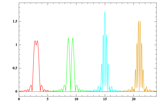
Figure 3: Modulus of MLWFs associated with the two occupied bands (left) and with the lowest two virtual bands (right).

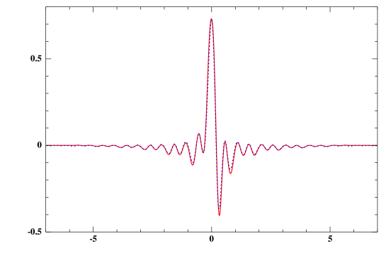
Figure 4: Density $\rho_{Q^{h}}$ obtained with 28 MLWFs (line in red). The reference is a supercell calculation in a basis set of size 1224 (dashed line in blue).

The nuclear local defect is taken of the form

$$\nu=(Z-1)\delta_{0.25}-Z\delta_{0}.$$

This corresponds to moving one nucleus and lowering its charge by one unit.

The first stage of the calculation consists in solving the cell problem. For simplicity, we use a uniform discretization of the Brillouin zone $(-\pi,\pi]$, and a plane wave expansion of the crystalline orbitals.

The second stage is the construction of MLWFs. For this purpose, we make use of an argument specific to the one-dimensional case [28]: the MLWFs associated with the spectral projector $\gamma$ are the eigenfunctions of the operator $\gamma x\gamma$. One first constructs $N_{e}$ mother MLWFs (taking $\gamma=\gamma^{0}_{\rm per}$), then $N_{a}$ mother MLWFs corresponding to the lowest $N_{a}$ virtual bands (taking for $\gamma$ the spectral projector associated with the lowest $N_{a}$ virtual bands). The so-obtained mother MLWFs are represented on Fig. 3.

The third stage consists in constructing a basis set $(\phi_{j})_{1\leq j\leq N_{b}}$ of $N_{b}=N_{v}(N_{e}+N_{a})$ MLWFs by selecting the $N_{v}$ translations of the $(N_{e}+N_{a})$ mother MLWFs that are closest to the local defect, and in computing the first-order density matrix of the form (15) which satisfies the constraints and minimizes the energy. The profile of the density $\rho_{Q^{h}}$ obtained with $Z=2$, $N_{e}=2$, $N_{a}=2$ and $N_{b}=28$ is displayed on Fig. 4. It is compared with a reference supercell calculation with 1224 plane wave basis functions. A fairly good agreement is obtained with very few MLWFs.

The implementation of our method in the Quantum Espresso suite of programs [29], in the true 3D Kohn-Sham setting, is work in progress [30].

References

References

- [1] Pisani C 1994 Phase Transitions 52 123
- [2] Kittel Ch 1987 Quantum Theory of Solids, Second Edition, Wiley
- [3] Stoneham A M 2001 Theory of Defects in Solids - Electronic Structure of Defects in Insulators and Semiconductors, Oxford University Press
- [4] Bernholc J, Ligari N O and Pantelides S T 1978 Phys. Rev. Lett. 41 895
- [5] Baraff G A and Schlüter M 1979 Phys. Rev. B 19 4965
- [6] Zeller R and Dederichs P H 1979 Phys. Rev. Lett. 42 1713
- [7] Kohn W and Sham L J 1965 Phys. Rev. 140 A1133
- [8] Pisani C (Ed.) 1996, Quantum-mechanical ab-initio calculation of the properties of crystalline materials, Lecture Notes in Chemistry, Springer
- [9] Probert M I J and Payne M C 2003 Phys. Rev. B 67 075204
- [10] Makov G and Payne M C 1995 Phys. Rev. B 51 4014
- [11] Schultz P A 2000 Phys. Rev. Lett. 84 1942
- [12] Cancès E, Deleurence A and Lewin M 2007 arXiv: math-ph/0702071
- [13] Chaix P and Iracane D 1989 J. Phys. B. 22 3791
- [14] Hainzl Ch, Lewin M, Séré E and Solovej J-P 2007 Phys. Rev. A 76 052104
- [15] Reed M and Simon B 1980 Methods of Modern Mathematical Physics, Vol I, Functional Analysis, Second Ed. Academic Press, New York
- [16] Hainzl Ch, Lewin M and Séré E 2005 Comm. Math. Phys. 257 515
- [17] Hainzl Ch, Lewin M and Séré E 2005 J. Phys. A: Math & Gen. 38 4483
- [18] Hainzl Ch, Lewin M and Séré E 2006 ArXiv:math-ph/0606001
- [19] Hainzl Ch, Lewin M and Solovej J-P 2007 Comm. Pure Applied Math. 60 546
- [20] Berezin F A 1966 The method of second quantization, Academic Press
- [21] Bach V, Lieb E H and Solovej J-P 1994, J. Statist. Phys. 76 3
- [22] Ruijsenaars S N M 1977 J. Math. Phys. 18 517
- [23] Shale D and Stinespring W F 1965 J. Math. and Mech. 14 315
- [24] Scharf G and Seipp H P 1982 Phys. Lett. 108B 196
- [25] Cancès E 2001 J. Chem. Phys. 114 10616
- [26] Kudin K N, Scuseria G E and Cancès E 2002 J. Chem. Phys. 116 8255
- [27] Marzari N and Vanderbilt D 1997 Phys. Rev. B 56 12847
- [28] Sgiarovello C, Peressi M and Resta R 2001 Phys. Rev. B 64 115202
- [29] http://www.quantum-espresso.org/
- [30] Dabo I, Cancès E and Lewin M, in preparation