Limit Laws for $k$-Coverage of Paths by a Markov-Poisson-Boolean Model

Srikanth K. Iyer ^,

Department of Mathematics, Indian Institute of Science, Bangalore, India.

D. Manjunath

Department of Electrical Engineering, Indian Institute of Technology Bombay, Mumbai, India.

D. Yogeshwaran

INRIA/ENS TREC, Ecole Normale Superieure, Paris, France.

Abstract

Let $P:=\{X_{i}\}_{i\geq 1}$ be a stationary Poisson point process in $\Re^{d},$ $\{C_{i}\}_{i\geq 1}$ be a sequence of i.i.d. random sets in $\Re^{d},$ and $\{Y_{i}^{t};\;t\geq 0\}_{i\geq 1}$ be i.i.d. $\{0,1\}$-valued continuous time stationary Markov chains. We define the Markov-Poisson-Boolean model ${\mathcal{C}}_{t}:=\{Y_{i}^{t}(X_{i}+C_{i}),i\geq 1\}.$ ${\mathcal{C}}_{t}$ represents the coverage process at time $t.$ We first obtain limit laws for $k$-coverage of an area at an arbitrary instant. We then obtain the limit laws for the $k$-coverage seen by a particle as it moves along a one-dimensional path.

AMS 1991 subject classifications:
            Primary: 60D05, 60G70
            Secondary: 05C05, 90C27
Keywords: Poisson-Boolean model, coverage, Markov process, sensor networks, target tracking.

1 Introduction

1.1 Motivation

This paper is motivated by the need to characterize the ability of a sensor network with randomly deployed unreliable sensor nodes to track the trajectory of a moving target in the sensor field. Since the nodes are randomly deployed, a suitable point process in a $d$-dimensional metric space, typically $\Re^{d}$ or $\mathcal{Z}^{d},$ can be used to describe the location of the sensor nodes. In this paper we will assume a homogenous Poisson point process for the distribution of sensor locations. A sensor node can detect events or perform measurements over a ‘sensing area’ or a ‘footprint.’ The coverage area of each sensor is described by a suitable sequence of random $d$-dimensional sets. Thus analyzing the coverage by the sensor network involves the analysis of an equivalent stochastic coverage process. Coverage analysis usually takes the form of obtaining statistics for the fraction of the volume of a $d$-dimensional set that is covered by one or more sensors, e.g., as in [1].

Tracking a moving target by a sensor network involves trajectory estimation from a sequence of position estimates of the target. The quality of the trajectory estimate will depend on the parts of the trajectory that are ‘covered’ by $k$ or more sensors with the value of $k$ being determined by the estimator used.

The sensor nodes are assumed to be unreliable in the sense that they toggle between two states—‘available’ and ‘not available.’ Hence some of the sensors that are covering the target as it is moving along the path could become unavailable during the coverage of the target. There are many reasons for this. A sensor could be turned off for energy saving or even energy restoration in the battery. Alternatively, a sensor may have temporarily failed. It could also be that the radio environment is such as to prevent a sensor from communicating with its neighbors, effectively making it unavailable for the sensing process. Since the nodes are unreliable, the coverage of the path during the motion of the target is a random process in time that is determined by the switching of the sensor states that could have covered the path. Thus we need to explicitly model the temporal behavior of the induced-coverage process of the path. We model this “on-off” behavior of the sensors by a two state Markov chain.

The aim of this paper is two-fold. We first extend the asymptotic coverage results in [1] to the case of general $k$-coverage. Asymptotic properties of the covered fraction are derived as the intensity of the Poisson point process becomes large and the coverage area of the individual sensors scaled down in such a way that the limiting process covers a non-trivial fraction of the operational area. The second objective is to show how the dynamics of the on-off process affects the coverage of a linearly moving target.

1.2 The Markov-Poisson-Boolean Model

Let $P:=\{X_{i},i=1,2,\ldots\}$ be a stationary Poisson process in $\Re^{d}$ of intensity $\lambda>0$. The points of $P$ can be thought of as locations of sensors in a random sensor network. Let $C$ be a random closed set in $\Re^{d}$ independent of $P$ and having an arbitrary distribution. Throughout the paper we assume that for some fixed $\tau>0,$ $C\subset B_{0,\tau},$ almost surely, where $B_{0,\tau}$ is a closed ball of radius $\tau$ centered at the origin. We will also assume that $\|C\|>0$ with probability 1, where $\|\cdot\|$ denotes the Lebesgue measure. Let $\beta=\mathsf{E}\!\left(\|C\|\right).$ Let $C_{i}$ be i.i.d. copies of $C$. As in [1], the $C_{i}$’s will be called shapes to distinguish them from the sets $(X_{i}+C_{i})$’s that denote the areas in $\Re^{d}$ that are covered by the sensors. The coverage process $\mathcal{C}\equiv\{X_{i}+C_{i},i\geq 1\}$ is called the Poisson-Boolean model [1]. Now let $Y=\{Y^{t},\;t\geq 0\}$ be a $\{0,1\}$-valued continuous time stationary Markov process independent of all other random variables. Let $\{Y^{t}_{i},t\geq 0\},i\geq 1$ be i.i.d. copies of $Y.$ $Y_{i}^{t}=1$ can be interpreted to mean that sensor $i$ is ‘on’ at time $t$ and is available for sensing and $Y_{i}^{t}=0$ means that it is ‘off’ at time $t$ and not available for sensing. Define the Markov-Poisson-Boolean model ${\mathcal{C}}_{t}:=\{Y_{i}^{t}(X_{i}+C_{i}),i\geq 1\}.$ ${\mathcal{C}}_{t}$ represents the coverage process by the available sensors at time $t.$ Let $R\subset\Re^{d}$ be an arbitrary Borel set. $R$ could correspond to the operational area of the sensor network. Now, consider a straight line path $\mathcal{L}$ in $R$ of length $L$ units, and an object moving along it with a constant velocity of $c$ units per second. The object starts moving at time $t=0.$ For any positive integer $k$, let $\zeta_{k}(t)$ be the indicator function for the object being ‘covered,’ to be made more precise later, by $k$ or more sensors at time $t.$ The objective of this paper is to characterize the random variables $\zeta_{k}(t)$ and $\int_{0}^{T}\zeta_{k}(t)dt$, where $T=L/c.$ In the rest of the paper, we refer to the Poisson-Boolean model and the Markov-Poisson-Boolean model as the PB and the MPB models respectively.

1.3 Previous Work

Coverage with reliable nodes, where nodes are always in the ‘available’ state, has been elaborated in both applied mathematics and sensor network literature. See [1] for a good comprehensive first study and [3] for some recent results for the case $k=1.$ In [10], $R$ is a square of side-length $\ell$ and $C$ is a circle of unit area. It is shown for this PB model, that if $\lambda$ is given by

$$\lambda=\log\ell^{2}+(k+1)\log\log\ell^{2}+c_{\ell},$$ (1)

and if $c_{\ell}\to\infty$ as $\ell\to\infty$, then $R$ is almost surely asymptotically $k$-covered.

Asymptotic coverage by unreliable sensor networks at an arbitrary epoch has been studied in [7, 2]. In the analysis of coverage by an unreliable sensor network at an arbitrary epoch, the stationary probability of a sensor node not being available essentially ‘thins’ the original deployment process and a standard analysis with the thinned process applies. However, for applications like target tracking or intruder detection, we need to know the behavior of the coverage process during the movement of the target. When the sensor nodes are unreliable, a node that was sensing the object may switch from being available to becoming unavailable, or vice versa. This implies that the coverage of a given point is not independent either in space or in time. Thus we need to consider the dynamics of the transitions from availability to non-availability of the sensors in the spatio-temporal analysis of the coverage of the path. The coverage of a line by a two-dimensional PB model was investigated in [4, 5].

1.4 Organization of the Paper and Summary of Results

In Section 2, we characterize $k$-coverage in $d$-dimensions. Although our eventual interest is the characterization of the coverage of a moving point on a path by the MPB model defined earlier, it is instructive to first consider the $k$-coverage of $R\subset\Re^{d},$ by the MPB model ${\mathcal{C}}_{t}$ at an arbitrary instant. At an arbitrary instant, let $V_{k}(R)$ be the volume of an arbitrary $d$-dimensional set $R\subset\Re^{d}$ that is not covered by $k$ or more sensors. We obtain a strong law and central limit theorem for $V_{k}(R)$. The proof techniques are in general similar to those in Chapter 3 of [1]. In the second part of Subsection 2.2, we consider the special case when the coverage areas are discs of fixed radius $r,$ and obtain a strong law of large numbers for the critical radius required for complete $k$-coverage in dimension $d=2$.

In Section 3, we consider the MPB model defined earlier, which is the PB model but now with unreliable sensors. We analyze the path coverage for a linearly moving target that is in the sensor field for $T$ units of time. Without loss of generality, let this interval be $(0,T).$ Let $V_{k,T}$ be the total time in $(0,T)$ that the target is not tracked by $k$ or more sensors. For pedagogic convenience we consider $k=1$ and obtain a strong law and central limit theorem for $V_{1,T}.$ The proof techniques of Section 2 can be combined with those of Section 3 to extend the results to the case of $k>1.$ We have separated $k$-coverage from the Markovian on-off dynamics to maintain clarity of exposition. Each of these two components operates independently in the computations and the expressions involving $k$-coverage are at times lengthy.

2 $k$-Coverage

2.1 Preliminaries

For a point $x\in\Re^{d}$, let $\chi_{m}(x)$ be the indicator variable that $x\in X_{i}+C_{i}$ for exactly $m$ points in $P,$ i.e.,

$$\chi_{m}(x)=\begin{cases}1&\mbox{if $x\in X_{i}+C_{i}$ for exactly $m$ of $i=1,2,\ldots$}\\ 0&\mbox{otherwise.}\end{cases}$$

$$\mathsf{E}\!\left(\chi_{m}(x)\right) = \mathsf{Pr}\left(x\in(X_{i}+C_{i})\mbox{ for exactly $m$ points}\right)$$ (2)

$$= \mathsf{Pr}\left(\mbox{for exactly $m$ points }X_{i}\in(x-C_{i})\right)$$

$$= \mathsf{Pr}\left(\mbox{for exactly $m$ points }X_{i}\in C_{i}\right).$$

The last equality follows from the stationarity of $P.$ Recall that $C_{i}\subset B_{0,\tau}$ and $\beta=\mathsf{E}\!\left(\|C\|\right).$ Given that $N$ points of $P$ lie within $B_{0,\tau},$ the probability that exactly $m$ of these points cover the origin is given by

$$\binom{N}{m}\left(1-\frac{\beta}{\|B_{0,\tau}\|}\right)^{N-m}\left(\frac{\beta}{\|B_{0,\tau}\|}\right)^{m}.$$

Since $N$ is Poisson with mean $\lambda\|B_{0,\tau}\|$, we obtain

$$\mathsf{E}\!\left(\chi_{m}(x)\right) = \mathsf{E}\!\left(\binom{N}{m}\left(1-\frac{\beta}{\|B_{0,\tau}\|}\right)^{N-m}\left(\frac{\beta}{\|B_{0,\tau}\|}\right)^{m}\right)\;\;=\;\;\frac{e^{-\beta\lambda}(\lambda\beta)^{m}}{m!}.$$ (3)

Let $R\in\Re^{d}$ be a $d$-dimensional set. For $k>0,$ we define the $k$-vacancy within $R$, $V_{k}(R),$ to be the $d$-dimensional volume of the part covered by at most $k-1$ random sets of $\mathcal{C},$ i.e.,

$$V_{k}(R)\equiv\sum_{m=0}^{k-1}\int_{R}\chi_{m}(x)\ dx.$$ (4)

The indicator variable for the $k$-vacancy of a point $x$ will be denoted by $V_{k}(x),$ i.e., $V_{k}(x):=\sum_{m=0}^{k-1}\chi_{m}(x).$ $\|R\|-V_{k}(R)$ will be called the $k$-coverage of $R$. Since $R$ is fixed throughout the paper, we will omit the reference to it in the notation and write $V_{k}(R)$ as $V_{k}$.

Some of the early derivations mimic that in [1] and we give it here for the sake of completeness. From (3) and Fubini’s theorem,

$$\mathsf{E}\!\left(V_{k}\right)\ =\ \sum_{m=0}^{k-1}\int_{R}\mathsf{E}\!\left(\chi_{m}(x)\right)dx=\sum_{m=0}^{k-1}\|R\|\frac{e^{-\lambda\beta}(\lambda\beta)^{m}}{m!}.$$ (5)

We now derive the variance of $V_{k}.$ If a point $x$ is covered by $X_{i},$ then $x\in X_{i}+C_{i}$ or $X_{i}\in x-C_{i}$. Similarly, if $x$ is not covered by $X_{i}$ then $X_{i}\in x-C_{i}^{c}$ where $C^{c}=\Re^{d}\setminus C.$ We use this to first obtain the probability that two points $x_{1}$ and $x_{2}$ are covered by exactly $m$ and $n$ sensors respectively which is then used to obtain the variance of $V_{k}.$ We make the following observations regarding the location of $X_{i}$ relative to points $x_{1}$ and $x_{2}.$

• If $X_{i}$ covers $x_{1}$ and $x_{2}$, then $X_{i}\in B_{1}^{i}(x_{1},x_{2}):=(x_{1}-C_{i})\cap(x_{2}-C_{i})$. Further, $\|B_{1}^{i}\|$ has the same distribution as $\|B_{1}\|$ where $B_{1}(x_{1}-x_{2})=(x_{1}-x_{2}+C)\cap C.$

• If $X_{i}$ covers $x_{1}$ and not $x_{2}$, then $X_{i}\in B_{2}^{i}(x_{1},x_{2}):=(x_{1}-C_{i})\cap(x_{2}-C^{c}_{i})$ and $\|B_{2}^{i}\|$ has the same distribution as $\|B_{2}\|$ where $B_{2}(x_{1}-x_{2})=(x_{1}-x_{2}+C)\cap C^{c}.$

• Similarly, if $X_{i}$ does not cover $x_{1}$ but covers $x_{2}$, then $X_{i}\in B_{3}^{i}(x_{1},x_{2}):=(x_{1}-C_{i}^{c})\cap(x_{2}-C_{i})$ and $\|B_{3}^{i}\|$ is equal to $\|B_{3}\|$ in distribution where $B_{3}(x_{1}-x_{2})=(x_{1}-x_{2}+C^{c})\cap C.$

We will suppress the argument of $B_{j}$ and $B_{j}^{i}$ unless required. Observe that the $B_{j}$ defined above are mutually disjoint sets. Further, $\|B_{2}\|$ and $\|B_{3}\|$ will have the same distribution.

$$\mathsf{E}\!\left(\chi_{m}(x_{1})\chi_{n}(x_{2})\right) = \mathsf{Pr}\left(\mbox{$x_{1}$ covered by $m$ \& $x_{2}$ covered by $n$ sensors}\right)$$

$$= \mathsf{Pr}\left(\mbox{$x_{1}\in X_{i}+C_{i}$ for $m$ sensors and $x_{2}\in X_{i}+C_{i}$ for $n$ sensors}\right)$$

$$= \mathsf{Pr}\left(\mbox{$X_{i}\in x_{1}-C_{i}$ for $m$ sensors and $X_{i}\in x_{2}-C_{i}$ for $n$ sensors}\right)$$

$$= \sum_{l=0}^{m\wedge n}\mathsf{Pr}\left(\mbox{$l$ cover $x_{1}$ \& $x_{2}$; $(m-l)$ cover only $x_{1}$; $(n-l)$ cover only $x_{2}$}\right).$$

We can proceed as in the derivation of (2) and (3) and consider a bounded set $A^{\prime}$ that contains $(x_{1}+B_{0,\tau})$ and $(x_{2}+B_{0,\tau})$. The ‘left’ point is designated $x_{1}$. Let $N$ be the number of points of the Poisson point process $P$ of intensity $\lambda$ lying in $A^{\prime}$. Then the probability that $(m-l)$ sensors cover $x_{1}$ only and $(n-l)$ cover $x_{2}$ only and $l$ sensors cover both is $\mathsf{Pr}\left(M_{1}=l,M_{2}=m-l,M_{3}=n-l,M_{4}=N-m-n+l\right)$ with

$$(M_{1},M_{2},M_{3},M_{4})\sim\mbox{ Multinomial}(N,a_{1},a_{2},a_{3},a_{4}=1-a_{1}-a_{2}-a_{3}),$$

where

$$a_{i} = \frac{\mathsf{E}\!\left(\|B_{i}\|\right)}{\|A^{\prime}\|},\qquad i=1,2,3.$$

Since $N$ is Poisson with mean $\lambda\|A^{\prime}\|$, the unconditional probability that $(m-l)$ sensors cover $x_{1}$ but not $x_{2}$, $(n-l)$ cover $x_{2}$ but not $x_{1}$, and $l$ sensors cover both $x_{1}$ and $x_{2}$ will be

$$\mathsf{E}\!\left(\frac{N!}{l!(m-l)!(n-l)!(N-m-n+l)!}a_{1}^{l}a_{2}^{(m-l)}a_{3}^{(n-l)}a_{4}^{(N-m-n+l)}\right)=\frac{\left(\lambda\mathsf{E}\!\left(\|B_{1}\|\right)\right)^{l}}{l!}e^{-\lambda\mathsf{E}\!\left(\|B_{1}\|\right)}$$

$$\times\frac{\left(\lambda\mathsf{E}\!\left(\|B_{2}\|\right)\right)^{m-l}}{(m-l)!}e^{-\lambda\mathsf{E}\!\left(\|B_{2}\|\right)}\frac{\left(\lambda\mathsf{E}\!\left(\|B_{3}\|\right)\right)^{n-l}}{(n-l)!}e^{-\lambda\mathsf{E}\!\left(\|B_{3}\|\right)}.$$

Hence from above calculations,

$$\mathsf{E}\!\left(\chi_{m}(x_{1})\chi_{n}(x_{2})\right) = \sum_{l=0}^{m\wedge n}\frac{\left(\lambda\mathsf{E}\!\left(\|B_{1}\|\right)\right)^{l}}{l!}e^{-\lambda\mathsf{E}\!\left(\|B_{1}\|\right)}\times\frac{\left(\lambda\mathsf{E}\!\left(\|B_{2}\|\right)\right)^{m-l}}{(m-l)!}e^{-\lambda\mathsf{E}\!\left(\|B_{2}\|\right)}$$ (6)

$$\hskip 21.68121pt\times\frac{\left(\lambda\mathsf{E}\!\left(\|B_{3}\|\right)\right)^{n-l}}{(n-l)!}e^{-\lambda\mathsf{E}\!\left(\|B_{3}\|\right)}$$

$$= e^{-2\lambda\beta}e^{\lambda\mathsf{E}\!\left(\|B_{1}\|\right)}\sum_{l=0}^{m\wedge n}\frac{\left(\lambda\mathsf{E}\!\left(\|B_{1}\|\right)\right)^{l}}{l!}\times\frac{\left(\lambda\mathsf{E}\!\left(\|B_{2}\|\right)\right)^{m+n-2l}}{(m-l)!(n-l)!}.$$

The last equality is obtained from the identities $\mathsf{E}\!\left(\|B_{1}\|+\|B_{2}\|\right)=\mathsf{E}\!\left(\|B_{1}\|+\|B_{3}\|\right)=\beta.$ We then have

$$\mathsf{Cov}\left(V_{k}(x_{1}),V_{k}(x_{2})\right) = \sum_{m,n=0}^{k-1}\mathsf{Cov}\left(\chi_{m}(x_{1}),\chi_{n}(x_{2})\right)$$ (7)

$$= \sum_{m,n=0}^{k-1}\left(\mathsf{E}\!\left(\chi_{m}(x_{1})\chi_{n}(x_{2})\right)-\mathsf{E}\!\left(\chi_{m}(x_{1})\right)\mathsf{E}\!\left(\chi_{n}(x_{2})\right)\right)$$

$$= e^{-2\lambda\beta}\sum_{m,n=0}^{k-1}\left(e^{\lambda\mathsf{E}\!\left(\|B_{1}(x_{1}-x_{2})\|\right)}\sum_{l=0}^{m\wedge n}\frac{\left(\lambda\mathsf{E}\!\left(\|B_{1}(x_{1}-x_{2})\|\right)\right)^{l}}{l!}\right.$$

$$\hskip 36.135pt\left.\times\frac{\left(\lambda E{\|B_{2}(x_{1}-x_{2})\|}\right)^{m+n-2l}}{(m-l)!(n-l)!}-\frac{\left(\lambda\beta\right)^{m+n}}{m!n!}\right),$$

and

$$\mathsf{VAR}\!\left(V_{k}\right)=\int_{R\times R}\mathsf{Cov}\left(V_{k}(x_{1}),V_{k}(x_{2})\right)\ dx_{1}\ dx_{2}.$$ (8)

2.2 Limit Laws

We are now ready to obtain the limit laws by letting $\lambda\rightarrow\infty$ and scaling the shapes by $\delta.$ Let $\mathcal{C}(\delta,\lambda)$ be the PB model $\mathcal{C}$ in which the shapes are scaled by $\delta$, i.e., the shapes have the same distribution as $\delta C.$ Let $V_{k}=V_{k}(\lambda,\delta)$ be the resulting $k$-vacancy in $R.$

Theorem 1.

If $\delta\to 0$ as $\lambda\to\infty$ such that $\delta^{d}\lambda\to\rho$ for $0\leq\rho<\infty$ in the scaled coverage process $C(\delta,\lambda)$, then

$$V_{k}\rightarrow\|R\|e^{-\rho\beta}\sum_{j=0}^{k-1}\frac{(\rho\beta)^{j}}{j!}\qquad\mbox{a.s.}$$

Theorem 2.

Consider the scaled coverage process $\mathcal{C}(\delta,\lambda)$. If $\delta\to 0$ as $\lambda\to\infty$ such that $\delta^{d}\lambda\to\rho$ where $0\leq\rho<\infty$, then

$$\mathsf{E}\!\left(V_{k}\right) \to \|R\|\sum_{m=0}^{k-1}\frac{e^{-\rho\beta}(\rho\beta)^{m}}{m!},$$ (9)

$$\mathsf{E}\!\left(|V_{k}-\mathsf{E}\!\left(V_{k}\right)|^{p}\right) \to 0~{}~{}~{}~{}~{}~{}~{}~{}~{}\mbox{for $1\leq p<\infty$},$$ (10)

$$\lambda\mathsf{VAR}\!\left(V_{k}\right) \to \sigma^{2},$$ (11)

where

$$\sigma^{2} = \rho\|R\|e^{-2\rho\beta}\left(\sum_{m,n=0}^{k-1}\int_{B_{0,2\tau}}\left(e^{\rho\mathsf{E}\!\left(\|B_{1}(y)\|\right)}\sum_{l=0}^{m\wedge n}\frac{\left(\rho\mathsf{E}\!\left(\|B_{1}(y)\|\right)\right)^{l}}{l!}\times\frac{\left(\rho\mathsf{E}\!\left(\|B_{2}(y)\|\right)\right)^{m+n-l}}{(m-l)!(n-l)!}\right.\right.$$ (12)

$$\left.-\left.\frac{\left(\rho\beta\right)^{m+n}}{m!n!}\right)dy\right).$$

Theorem 3.

If $\delta\to 0$ as $\lambda\to\infty$ such that $\delta^{d}\lambda\to\rho$ for $0\leq\rho<\infty$ in the scaled coverage process $C(\delta,\lambda)$, then

$$\sqrt{\lambda}\left(V_{k}-\mathsf{E}\!\left(V_{k}\right)\right)\rightarrow N(0,\sigma^{2}),$$

in distribution where $\sigma^{2}$ is as defined in (12).

It follows from Theorem 1 that if $\delta^{d}\lambda\rightarrow\infty$, then $V_{k}\rightarrow 0$ almost surely. However, note that Theorems 1 and  2 do not guarantee complete coverage with high probability for large enough $\lambda.$ We now consider such a requirement, key to which is the inequality (13) below.

For the following two theorems, we assume that $d=2$, the operational area $R$ to be the unit square $[0,1]^{2},$ and the sensing areas to be discs of radius $r>0$ satisfying $\pi r^{2}\leq 1$. This last requirement is only to give a compact expression in the inequality below. Since our interest is in the asymptotic behavior of the coverage process as $\lambda\to\infty$ and $r=r_{\lambda}\to 0,$ this is satisfied for all large enough $\lambda.$ For any $\lambda,r>0$ define the event $Z_{\lambda}(r):=\{V_{k}(\lambda,r)>0\}$. For radii $r_{\lambda}>0$ which are decreasing in $\lambda$ to zero, we shall abbreviate $Z_{\lambda}(r_{\lambda})$ by $Z_{\lambda}$. We have the following inequality.

$$\frac{1}{1+\theta}\,\leq\,\mathsf{Pr}\left(Z_{\lambda}(r)\right)\leq 2e^{-\lambda\pi r^{2}}\left(1+\lambda^{2}\pi r^{2}(1+\frac{2}{\lambda\pi r})\sum_{i=0}^{k-1}\frac{(\lambda\pi r^{2})^{i}}{i!}\right),$$ (13)

where

$$\theta=\frac{4(k+1)!}{e^{-\lambda\pi r^{2}}\lambda(\lambda\pi r^{2})^{k}}.$$

A formal proof of (13) is given in the appendix. The above inequality is an extension of Theorem 3.11 of [1] for $k>1$. A similar inequality is derived in [10] (proof of Theorem 1) under the condition that the operational area $R$ is a square of side length $\ell\to\infty$, with intensity $\lambda=\lambda(\ell)\to\infty$ (see (1)) and the sensing area of the sensors is one, i.e., $\pi r^{2}=1.$ The following result follows immediately from (13).

Theorem 4.

Suppose that $d=2,$ and let $r_{\lambda}^{2}=\frac{\log\lambda+k\log\log\lambda+c(\lambda)}{\pi\lambda}.$ As $\lambda\rightarrow\infty$, $\mathsf{Pr}\left(Z_{\lambda}\right)\rightarrow 0$ if $c(\lambda)\rightarrow\infty.$ Further, if $c(\lambda)\rightarrow c\in\Re$, then $\mathsf{Pr}\left(Z_{\lambda}\right)>c_{1}$ for some constant $c_{1}\in(0,1)$.

Theorem 4 gives the critical radius required for complete $k$-coverage with probability approaching $1$ in two dimensions. We now show that by taking the radius to be a bit larger than that obtained from Theorem 4, we can get a stronger and more stable complete coverage regime. The following discussion will become easier if we assume $\lambda=n$ where $n$ is an integer. To make the above notion of strong complete coverage more precise, define the critical radius for complete coverage as

$$r^{\ast}_{n}:=\inf\{r_{n}>0:V_{k,s}(n,r_{n})=0\},$$ (14)

where $V_{k,s}$ is the $k$-vacancy in the unit square.

Theorem 5.

Let $d=2,$ and let $V_{k,s}$ be the vacancy in the unit square. Let $r_{n}^{\ast}$ be as defined above. Then, almost surely,

$$\lim_{n\rightarrow\infty}\frac{\pi n(r_{n}^{\ast})^{2}}{\log n+k\log\log n}=1.$$ (15)

Remark: Let $0<\epsilon<1.$ The above result implies that by taking the radius

$$r_{n}^{2}=(1+\epsilon)\frac{\log n+k\log\log n}{\pi n},$$ (16)

the unit square will be almost surely, completely $k$-covered for all $n$ large enough. Thus, if $n$ is large, by taking the above $r_{n}$, which is eventually larger than the one given in Theorem 4, we can ensure a complete $k$-coverage regime that will not see vacancies even if the number of sensors is increased (with corresponding decrease in $r_{n}$). Further, the above result gives a strong threshold in the sense that if

$$r_{n}^{2}=(1-\epsilon)\frac{\log n+k\log\log n}{\pi n},$$ (17)

then the unit square will not be completely $k$-covered for all large enough $n$, almost surely.

2.3 Proofs

Proof of Theorem 1: To obtain the required result, first note that for the $k$-vacancy in a unit cube $D,$ $V_{k}(D),$ the expectation is given by $\mathsf{E}\!\left(V_{k}(D)\right)=e^{-\rho\beta}\sum_{j=0}^{k-1}\frac{(\rho\beta)^{j}}{j!}$. Now observe that the two scaling regimes—(1) $R$ is fixed with $\lambda\delta^{d}\rightarrow\rho$ and (2) $\delta=1$, $R_{l}=lR$, and $l\rightarrow\infty$ with $P$ being a Poisson point process of intensity $\rho$ are equivalent. See Section 3.4 of [1] for more discussion on this. Theorem 1 follows using the same steps as in the proof of Theorem 3.6 in [1]. ∎

Proof of Theorem 2: Since the sequence $\{V_{k}(\delta,\lambda)\}_{\delta\geq 0,\lambda\geq 0}$ is bounded, (9) and (10) follow from Theorem 1.

(11) follows from (7), (8) if $\lambda\int_{R\times R}\mathsf{Cov}\left(\chi_{m}(x_{1}),\chi_{n}(x_{2})\right)dx_{1}\,dx_{2}$ converges to the product of the integral on the r.h.s of (12) and $\left(\rho\|R\|e^{-2\rho\beta}\right).$ This is shown below.

Let $B_{1}^{\delta}(y)=(y+\delta C)\cap\delta C$ and $B_{2}^{\delta}(y)=(y+\delta C)\cap\delta C^{c}$. Making first the change of variable $x=x_{1}$ and $y=x_{1}-x_{2}$ in (7) and then $y$ to $\delta y$, we get

$$\lambda\int_{R}\int_{x-R}\mathsf{Cov}\left(\chi_{m}(x),\chi_{n}(x_{2})\right)dx_{2}\,dx$$

$$= \lambda\int_{R}\int_{x-R}e^{-2\lambda\delta^{d}\beta}\sum_{m,n=0}^{k-1}\left(e^{\lambda\mathsf{E}\!\left(\|B^{\delta}_{1}(y)\|\right)}\sum_{l=0}^{m\wedge n}\frac{\left(\lambda\mathsf{E}\!\left(\|B^{\delta}_{1}(y)\|\right)\right)^{l}}{l!}\times\right.$$

$$\hskip 36.135pt\left.\frac{\left(\lambda\mathsf{E}\!\left(\|B^{\delta}_{2}(y)\|\right)\right)^{m+n-2l}}{(m-l)!(n-l)!}-\frac{\left(\lambda\beta\right)^{m+n}}{m!n!}\right)dy\ dx$$

$$= \lambda\int_{R}\int_{x-R}e^{-2\lambda\delta^{d}\beta}\sum_{m,n=0}^{k-1}\left(e^{\lambda\delta^{d}\mathsf{E}\!\left(\|B_{1}(\delta^{-1}y)\|\right)}\sum_{l=0}^{m\wedge n}\frac{\left(\lambda\delta^{d}\mathsf{E}\!\left(\|B_{1}(\delta^{-1}y)\|\right)\right)^{l}}{l!}\times\right.$$

$$\hskip 36.135pt\left.\frac{\left(\lambda\delta^{d}\mathsf{E}\!\left(\|B_{2}(\delta^{-1}y)\|\right)\right)^{m+n-2l}}{(m-l)!(n-l)!}-\frac{\left(\lambda\delta^{d}\beta\right)^{m+n}}{m!n!}\right)dy\ dx$$

$$= \lambda\delta^{d}e^{-2\delta^{d}\lambda\beta}\int_{R}\ \int_{\delta^{-1}(x-R)}\left(e^{\delta^{d}\lambda\mathsf{E}\!\left(\|B_{1}(y)\|\right)}\sum_{l=0}^{m\wedge n}\frac{\left(\delta^{d}\lambda\mathsf{E}\!\left(\|B_{1}(y)\|\right)\right)^{l}}{l!}\times\frac{\left(\delta^{d}\lambda\mathsf{E}\!\left(\|B_{2}(y)\|\right)\right)^{m+n-2l}}{(m-l)!(n-l)!}\right.$$ (18)

$$\hskip 36.135pt\left.-\frac{\left(\delta^{d}\lambda\beta\right)^{m+n}}{m!n!}\right)dy\ \ dx$$

$$= \lambda\delta^{d}e^{-2\delta^{d}\lambda\beta}\int_{R}\ f_{\delta}(x)\ dx,$$

where

$$f_{\delta}(x) := \int_{\delta^{-1}(x-R)\cap B_{0,2\tau}}\left(e^{\delta^{d}\lambda\mathsf{E}\!\left(\|B_{1}(y)\|\right)}\sum_{l=0}^{m\wedge n}\frac{\left(\delta^{d}\lambda\mathsf{E}\!\left(\|B_{1}(y)\|\right)\right)^{l}}{l!}\times\frac{\left(\delta^{d}\lambda\mathsf{E}\!\left(\|B_{2}(y)\|\right)\right)^{m+n-2l}}{(m-l)!(n-l)!}\right.$$ (19)

$$\hskip 36.135pt\left.-\frac{\left(\delta^{d}\lambda\beta\right)^{m+n}}{m!n!}\right)dy.$$

$f_{\delta}(x)$ as well as the integrand in (19) are uniformly bounded, since for any $\epsilon>0$ and all $\lambda>0$ sufficiently large, we have $\delta^{-1}(x-R)\cap B_{0,2\tau}\subset B_{0,2\tau}$, $|\delta^{d}\lambda-\rho|\leq\epsilon$ and $B_{i}\subset B_{0,\tau}.$ Therefore, from (18), (19) and the dominated convergence theorem, we have

$$f_{\delta}(x) \to c_{0}:=\int_{B_{0,2\tau}}\left(e^{\rho\mathsf{E}\!\left(\|B_{1}(y)\|\right)}\sum_{l=0}^{m\wedge n}\frac{\left(\rho\mathsf{E}\!\left(\|B_{1}(y)\|\right)\right)^{l}}{l!}\times\frac{\left(\rho\mathsf{E}\!\left(\|B_{2}(y)\|\right)\right)^{m+n-2l}}{(m-l)!(n-l)!}-\frac{\left(\rho\beta\right)^{m+n}}{m!n!}\right)dy,$$

and

$$\lambda\int_{R\times R}\mathsf{Cov}\left(\chi_{m}(x_{1})\chi_{n}(x_{2})\right)\ dx_{1}\ dx_{2}\rightarrow\rho e^{-2\rho\beta}\int_{R}c_{0}\ dx=\rho e^{-2\rho\beta}c_{0}\|R\|,$$

as $\lambda\rightarrow\infty.$ This proves (11). ∎

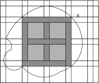
Figure 1: Figure shows the sets $A_{1}$, $A_{2}$ and $A_{3}.$ The squares are shaded light gray. The squares are of length $\tau r\delta$ and the ‘spacings’ between the sqaures are of width $2\tau\delta$. The light gray shaded region within $R$ is $A_{1}$, the darker region within $R$ is $A_{2}$ and the unshaded region within $R$ is $A_{3}$ (Adapted from [1]).

Proof of Theorem 3: Let $r$ be a large positive constant. Divide all of $\Re^{d}$ into a regular lattice of $d$-dimensional cubes of side length $(\tau r\delta),$ with each cube separated from its adjacent cubes by a $d$-dimensional ‘spacing’ of width $2\tau\delta.$ Let $A_{1}$ denote the union of those cubes which are wholly within $R,$ $A_{2}$ the union of the spacings that are wholly contained in $R$ and $A_{3}$ the intersection of $R$ with all those cubes and spacings that are only partially within $R$. Fig. 1 illustrates these sets for $d=2.$ Since $A_{1},$ $A_{2}$ and $A_{3}$ form a partition of $R$, the vacancy $V_{k}$ within $R$ may be written as,

$$V_{k}=V^{(1)}_{k}+V^{(2)}_{k}+V^{(3)}_{k},$$

where $V^{(i)}_{k}$ is the $k$-vacancy within the region $A_{i}.$ Under the assumptions of the theorem, as $\delta\to 0,$ the cubes get finer. Further the number of spacings is less than $\|R\|/(r\tau\delta)^{d}.$ Since the volume of the ‘spacings’ is $(\tau r\delta)^{d-1}\times(2\tau\delta),$ we have

$$\|A_{3}\|\rightarrow 0,\qquad\mbox{ and }\qquad\|A_{2}\|\leq 2\|R\|r^{-1}.$$ (21)

From (8), we get

$$\mathsf{VAR}\!\left(V^{(i)}_{k}\right) = \sum_{m,n=0}^{k-1}\int_{A_{i}}dx_{1}\int_{A_{i}}\mathsf{Cov}\left(\chi_{m}(x_{1})\chi_{n}(x_{2})\right)dx_{2}$$ (22)

$$= \delta^{d}\sum_{m,n=0}^{k-1}\int_{A_{i}}e^{-2\delta^{d}\lambda\beta}f_{\delta}(x_{1})dx_{1}\leq M\delta^{d}k^{2}\|A_{i}\|,$$

where the last inequality follows from (LABEL:conv_f_delta). From the inequality above and (21), we get

$$\lim_{\lambda\rightarrow\infty}\lambda\mathsf{VAR}\!\left(V^{(3)}_{k}\right)=0.$$ (23)

From (21) and (22), we also get

$$\lim_{r\rightarrow\infty}\limsup_{\lambda\rightarrow\infty}\lambda\mathsf{VAR}\!\left(V^{(2)}_{k}\right)=0.$$ (24)

Thus, for any $\epsilon>0,$ we can choose $r$ large enough so that $\lambda\mathsf{VAR}\!\left(V^{(2)}_{k}\right)<\epsilon,$ for all $\lambda$ sufficiently large. Hence in order to obtain the central limit theorem that we are seeking, we need to concentrate on $V^{(1)}_{k}$ and obtain a central limit theorem for it. Since $\lambda\mathsf{VAR}\!\left(V_{k}\right)\rightarrow\sigma^{2}$ from (11), we need to show the following.

$$\frac{V^{(1)}_{k}-\mathsf{E}\!\left(V^{(1)}_{k}\right)}{\left(\mathsf{VAR}\!\left(V^{(1)}_{k}\right)\right)^{1/2}}\stackrel{{\scriptstyle d}}{{\rightarrow}}N(0,1),\qquad\lim_{r\rightarrow\infty}\limsup_{\lambda\rightarrow\infty}|\lambda(\mathsf{VAR}\!\left(V^{(1)}_{k}\right)-\mathsf{VAR}\!\left(V_{k}\right))|=0.$$ (25)

Let $n=n(\lambda)$ denote the number of cubes of side-length $\tau r\delta$ in $A_{1}$, and let $D_{i}$ denote the $i$-th such cube, $1\leq i\leq n.$ Denoting the $k$-vacancy in $D_{i}$ by $U_{i}$, we have $V^{(1)}_{k}=\sum_{i}U_{i}$. Under the scaling regime, each shape is contained in $B_{0,\tau\delta}$ and the spacing between the cubes is $2\tau\delta$, and so no shape can intersect more than one cube. Hence, given $\lambda,$ the $U_{i}^{\prime}$s are independently distributed and we have

$$\mathsf{VAR}\!\left(V^{(1)}_{k}\right)=\sum_{i}\mathsf{VAR}\!\left(U_{i}\right)=n\mathsf{VAR}\!\left(U_{1}\right).$$

Let $D$ be a $d$-dimensional cube of side $\tau r$ with the same orientation as $D_{1}$. For any two real sequences $a_{n},b_{n}$ $a_{n}\sim b_{n}$ implies that $a_{n}/b_{n}\to 1$ as $n\to\infty.$ From (7), (8) we can write

$$\mathsf{VAR}\!\left(V^{(1)}_{k}\right) = ne^{-2\delta^{d}\lambda\beta}\sum_{m,n=0}^{k-1}\int\int_{D_{1}\times D_{1}}\left(e^{\lambda\mathsf{E}\!\left(\|(x_{1}-x_{2}+\delta S)\cap\delta S\|\right)}\sum_{l=0}^{m\wedge n}\frac{\left(\lambda\mathsf{E}\!\left(\|(x_{1}-x_{2}+\delta S)\cap\delta S\|\right)\right)^{l}}{l!}\right.$$ (26)

$$\left.\times\frac{\left(\lambda\mathsf{E}\!\left(\|(x_{1}-x_{2}+\delta S)\cap(\delta S)^{c}\|\right)\right)^{m+n-2l}}{(m-l)!(n-l)!}-\frac{\left(\delta^{d}\lambda\beta\right)^{m+n}}{m!n!}\right)dx_{1}dx_{2}$$

$$\sim n\delta^{2d}e^{-2\rho\beta}\sum_{m,n=0}^{k-1}\int\int_{D\times D}\left(e^{\rho\mathsf{E}\!\left(\|B_{1}\|\right)}\sum_{l=0}^{m\wedge n}\frac{\left(\rho\mathsf{E}\!\left(\|B_{1}\|\right)\right)^{l}}{l!}\times\frac{\left(\rho\mathsf{E}\!\left(\|B_{2}\|\right)\right)^{m+n-2l}}{(m-l)!(n-l)!}\right.$$

$$\left.-\frac{\left(\rho\beta\right)^{m+n}}{m!n!}\right)dx_{1}dx_{2}.$$

The rest of the proof follows as in ([1] pp. 157-158). ∎

Proof of Theorem 15: Recall that $Z_{n}(r_{n})=\{V_{k}(n,r_{n})>0\}.$ Suppose we show that for the choice of $r_{n}$ as in (16), we have $\mathsf{Pr}\left(Z_{n}(r_{n})\mbox{ infinitely often }\right)=0,$ then it follows that

$$\limsup_{n\rightarrow\infty}\frac{\pi n(r_{n}^{\ast})^{2}}{\log n+k\log\log n}\leq 1.$$ (27)

On the other hand, for the choice of $r_{n}$ as in (17), if we show that $\mathsf{Pr}\left(Z_{n}^{c}(r_{n})\mbox{ infinitely often }\right)=0,$ then we can conclude that

$$\liminf_{n\rightarrow\infty}\frac{\pi n(r_{n}^{\ast})^{2}}{\log n+k\log\log n}\geq 1.$$ (28)

First we show (27). Take subsequence $n_{j}=j^{a},$ where $a>0$ will be chosen appropriately later. Define the events $E_{j}=\cup_{n=n_{j}}^{n_{j+1}}Z_{n}(r_{n})\subset Z_{n_{j}}(r_{n_{j+1}}).$ Then, $\mathsf{Pr}\left(E_{j}\right)\leq\mathsf{Pr}\left(Z_{n_{j}}(r_{n_{j+1}})\right)$.

For $r_{n}$ as in (16), observe that $n_{j}r_{n_{j+1}}^{2}\rightarrow\infty.$ Hence, from (13), we get, for large enough $j$,

$$\mathsf{Pr}\left(Z_{n_{j}}(r_{n_{j+1}})\right)\leq\zeta_{1}ke^{-n_{j}\pi r_{n_{j+1}}^{2}}n_{j}(n_{j}\pi r_{n_{j+1}}^{2})^{k},$$

where $\zeta_{1}$ is some constant. Choose $\eta>(1+\epsilon)^{-1}.$ Since $n_{j}/n_{j+1}\uparrow 1,$ as $j\rightarrow\infty,$ we have for all large enough $j$, $n_{j}/n_{j+1}\geq\eta.$ Hence, $\eta(1+\epsilon)\log n_{j+1}\leq n_{j}\pi r_{n_{j+1}}^{2}\leq 4\log n_{j+1},$ so that

$$\mathsf{Pr}\left(Z_{n_{j}}(r_{n_{j+1}})\right)\leq\zeta_{2}e^{-\eta(1+\epsilon)\log n_{j+1}}(\log n_{j+1})^{k}n_{j}\leq\zeta_{3}(\log j)^{k}(j+1)^{-a(\eta(1+\epsilon)-1)},$$

where $\zeta_{2},\zeta_{3}$ are constants that depend on $a,k,\epsilon.$ Thus for $a$ large enough we get $\sum_{j=1}^{\infty}\mathsf{Pr}\left(E_{j}\right)<\infty.$ By the Borel-Cantelli Lemma, $E_{j}$ happens only finitely often almost surely. By the definition of $E_{j}$, this implies that $\mathsf{Pr}\left(Z_{n}(r_{n})\mbox{ infinitely often }\right)=0.$

Similarly using the lower bound for $\mathsf{Pr}\left(Z_{n}\right)$, we can prove (28). As above, let $n_{j}=j^{a}$, $j\geq 1$ and $a>0$ to be chosen later. Let $r_{n}$ be as in (17). Using the lower bound in (13), we get

$$\mathsf{Pr}\left(\cup_{n=n_{j}}^{n_{j+1}}Z_{n}^{c}(r_{n})\right)\leq\mathsf{Pr}\left(Z_{n_{j+1}}^{c}(r_{n_{j}})\right)\leq\frac{\theta_{j}}{1+\theta_{j}}\leq\theta_{j},$$

where

$$\theta_{j}=\frac{4(k+1)!}{e^{-n_{j+1}\pi r_{n_{j}}^{2}}n_{j+1}(n_{j+1}\pi r_{n_{j}}^{2})^{k}}.$$

Proceeding as in the proof of the upper bound, we can show that the above probability is summable. This completes the proof of the theorem. ∎

3 Path Coverage in the Markov-Poisson-Boolean Model

3.1 Preliminaries

Let $\mathcal{C}_{t}=\{Y_{i}^{t}(X_{i}+C_{i}),i\geq 1\}$ be the MPB model as defined in Section 1.2. Recall that $\{Y^{t}_{i},t\geq 0\}$ are i.i.d. copies of $\{Y^{t},t\geq 0\}$ which is a $\{0,1\}$-valued continuous time stationary Markov process. The sets $C_{i}$ are independent and distributed as $C$ satisfying $C\subset B_{0,\tau}$ for some fixed $\tau>0$. Let $\mu_{0}$ be the transition rate from the $0$-state to the $1$-state and $\mu_{1}$ the transition rate from $1$-state to the $0$-state. This of course means that in each visit, $Y^{t}$ is in the $0$ and $1$ states for exponentially distributed times with parameters $\mu_{0}$ and $\mu_{1}$ respectively. Then, (see [6], Chapter 6), the stationary probability of the sensor being in state $j$ is given by $p_{j}:=\mathsf{Pr}\left(Y^{t}=j\right)=\frac{\mu_{1-j}}{\mu_{1}+\mu_{0}}$, $j\in\{0,1\}.$ The transition probabilities between the states are defined by $p_{t}(j,k):=\mathsf{Pr}\left(Y^{s+t}=k|Y^{s}=j\right)$ for $j,k\in\{0,1\}.$ It can be shown that

$$p_{t}(j,j)=(1-p_{j})e^{-\gamma t}+p_{j},$$

where $\gamma=\mu_{0}+\mu_{1}$ and $p_{t}(j,k)=1-p_{t}(j,j)$ for $j,k\in\{0,1\}$ and $j\neq k.$

Now, consider a target moving on a straight line path in $\Re^{d}$ of length $L$ units with a velocity of $c$ units per second. As in the previous section, we will let $X_{i}=(X^{1}_{i},X^{2}_{i},\ldots,X^{d}_{i})$ be a point in $\Re^{d}.$ Without loss of generality, we can consider the target to be moving along a coordinate axis, say $X^{1},$ for $T:=L/c$ units of time. Define ${\underline{s}}:=(cs,0,\ldots,0)\in\Re^{2},$ where $s\in\Re^{+}.$ ${\underline{s}}$ is the position of the target on the $X^{1}$-axis at time $s.$ Let $\zeta(s)$ be the indicator variable for the target being covered by one or more of the sets $C_{i}$ at time $s,$ and $V_{T}=V_{1,T}$ be the random variable denoting the duration for which the target is not covered in $[0,T]$, i.e.,

$$V_{T}:=\int_{0}^{T}(1-\zeta(s))\ ds.$$ (29)

The effect of the transitions of $Y^{t}_{i}$ makes the study of $V_{T}$ interesting. We first calculate the expectation and variance of $V_{T}$. Since the $Y^{t}_{i}$ are stationary, the expectation of $V_{T}$ is straightforward and is given by

$$\mathsf{E}\!\left(V_{T}\right)=\int_{0}^{T}\mathsf{Pr}\left({\underline{s}}\notin{\mathcal{C}}_{s}\right)ds=Te^{-\lambda p_{1}\beta},$$ (30)

where $\beta=\mathsf{E}\!\left(\|C\|\right).$ The second moment of $V_{T}$ can be obtained from

$$\mathsf{E}\!\left(V_{T}^{2}\right) = \int_{0}^{T}\int_{0}^{T}\mathsf{Pr}\left({\underline{s}}_{1}\notin{\mathcal{C}}_{s_{1}},{\underline{s}}_{2}\notin{\mathcal{C}}_{s_{2}}\right)\ ds_{1}\ ds_{2}$$

$$= 2\int_{0}^{T}\int_{s_{1}}^{T}\mathsf{Pr}\left({\underline{s}}_{1}\notin{\mathcal{C}}_{s_{1}},{\underline{s}}_{2}\notin{\mathcal{C}}_{s_{2}}\right)\ ds_{1}\ ds_{2}.$$

We now evaluate this integral. Define $B_{1}({\underline{s}}_{1},{\underline{s}}_{2}):=({\underline{s}}_{1}+C)\cap({\underline{s}}_{2}+C),$ $B_{2}({\underline{s}}_{1},{\underline{s}}_{2}):=({\underline{s}}_{1}+C)\cap({\underline{s}}_{2}+C)^{c}$ and $B_{3}({\underline{s}}_{1},{\underline{s}}_{2}):=({\underline{s}}_{2}+C)\cap({\underline{s}}_{1}+C)^{c}.$ From this definition, $B_{1},$ $B_{2}$ and $B_{3}$ are disjoint and we can see that $\|B_{2}\|$ and $\|B_{3}\|$ have the same distribution and $\|B_{1}\|=\|({\underline{s}}_{1}-{\underline{s}}_{2}+C)\cap C\|$. We will suppress the obvious arguments of the sets $B_{i}$. As in the arguments leading to (6), we consider a set $A^{\prime}=B_{{\underline{s}}_{1},2\tau}\cup B_{{\underline{s}}_{2},2\tau}$ and assume there are $N$ sensors within $A^{\prime}$. Then the integrand in the above equation is

$$\mathsf{Pr}\left(\mbox{0 on sensors covering ${\underline{s}}_{1}$ at $s_{1}$; 0 on sensors covering ${\underline{s}}_{2}$ at $s_{2}$}\right),$$

which equals $\mathsf{Pr}\left(M_{1}=0,M_{2}=0,M_{3}=0,M_{4}=N\right)$, where $M_{1}=$ no: of sensors active at $s_{1}$ or $s_{2}$ among those in $A^{\prime}$ which can cover ${\underline{s}}_{1}$ and ${\underline{s}}_{2}$, $M_{2}=$ no: of sensors active at $s_{1}$ among those in $A^{\prime}$ which can cover ${\underline{s}}_{1}$ and not ${\underline{s}}_{2}$, $M_{3}=$ no: of sensors active at $s_{2}$ among those in $A^{\prime}$ which can cover ${\underline{s}}_{2}$ and not ${\underline{s}}_{1}$, $M_{4}=$ remaining sensors in $A^{\prime}$. Now note that

$$(M_{1},M_{2},M_{3},M_{4})\sim\mbox{ Multinomial}(N,a_{1},a_{2},a_{3},a_{4}=1-a_{1}-a_{2}-a_{3}),$$

where

$$a_{1} = (1-p_{0}p_{s_{2}-s_{1}}(0,0))\mathsf{E}\!\left(\|B_{1}\|\right)/\|A^{\prime}\|,$$

$$a_{2} = p_{1}\mathsf{E}\!\left(\|B_{2}\|\right)/\|A^{\prime}\|,$$

$$a_{3} = p_{1}\mathsf{E}\!\left(\|B_{3}\|\right)/\|A^{\prime}\|.$$

$a_{1}$ is the probability that a sensor can cover both of ${\underline{s}}_{1}$ and ${\underline{s}}_{2}$ and is active at either $s_{1}$ or $s_{2}$. It is the product of probabilities of a sensor lying in $B_{1}$ and making the desired transition of states. The first probability is $\mathsf{E}\!\left(\|B_{1}\|\right)/\|A^{\prime}\|$. The second probability is obtained as follows:

$$\mathsf{Pr}\left(\mbox{a given sensor is on at $s_{1}$ or $s_{2}$}\right) = \mathsf{Pr}\left(\mbox{the sensor is on at $s_{1}$}\right)$$

$$+\mathsf{Pr}\left(\mbox{the sensor is off at $s_{1}$ and on at $s_{2}$}\right)$$

$$= p_{1}+p_{0}p_{s_{2}-s_{1}}(0,1)=1-p_{0}p_{s_{2}-s_{1}}(0,0).$$

The remaining $a_{i}$’s are even simpler to obtain by similar calculations. Since $N$ follows a Poisson distribution with mean $\lambda\|A^{\prime}\|$, the integrand in the above expression for $\mathsf{E}\!\left(V_{T}^{2}\right)$ is given by

$$\sum_{\ell=0}^{\infty}a_{4}^{\ell}\frac{(\lambda\|A^{\prime}\|)^{\ell}}{\ell!}e^{-\lambda\|A^{\prime}\|}=e^{-\lambda(a_{1}+a_{2}+a_{3})\|A^{\prime}\|}.$$

$$\mathsf{E}\!\left(V_{T}^{2}\right) = 2\int_{0}^{T}\int_{s_{1}}^{T}\left(e^{-\lambda p_{1}\mathsf{E}\!\left(\|B_{2}\|\right)}\right)\left(e^{-\lambda p_{1}\mathsf{E}\!\left(\|B_{3}\|\right)}\right)\left(e^{-\lambda\mathsf{E}\!\left(\|B_{1}\|\right)(1-p_{0}p_{s_{2}-s_{1}}(0,0))}\right)ds_{2}\;ds_{1}$$

$$= 2\int_{0}^{T}\int_{s_{1}}^{T}e^{-2p_{1}\lambda\beta}e^{-\lambda\mathsf{E}\!\left(\|B_{1}\|\right)(1-2p_{1}-p_{0}p_{s_{2}-s_{1}}(0,0))}ds_{2}\;ds_{1}.$$

Hence,

$$\mathsf{VAR}\!\left(V_{T}\right) = \mathsf{E}\!\left(V_{T}^{2}\right)-(\mathsf{E}\!\left(V_{T}\right))^{2}$$ (31)

$$= 2e^{-2p_{1}\lambda\beta}\int_{0}^{T}\int_{s_{1}}^{T}\left(e^{-\lambda\mathsf{E}\!\left(\|B_{1}\|\right)(1-p_{0}p_{s_{2}-s_{1}}(0,0)-2p_{1})}-1\right)ds_{2}\;ds_{1}.$$

Observe from (30) that the expected coverage depends neither on the shapes of the sensing regions nor on the transition probabilities of the on-off process. Their effects are picked up only in the variance of the coverage as can be seen in (31).

3.2 Limit Laws

We can now delineate the scaling laws. Let ${\mathcal{C}}_{t}(\delta,\lambda)$ be the process ${\mathcal{C}}_{t}$ in which the shapes $C$ are scaled by $\delta.$ In addition, the parameters of the Markov chain governing the on-off process will also be made to depend on $\delta$. Without loss of generality, let $\mu_{0}(\delta),\mu_{1}(\delta)$ be such that $\mu_{0}(\delta)/\mu_{1}(\delta)\equiv\mu_{0}/\mu_{1}$ for all $\delta.$ It can be easily seen that the proofs remain valid when $\mu_{0}(\delta)/\mu_{1}(\delta)\rightarrow\mu_{0}/\mu_{1}$ as $\delta\rightarrow 0.$ Hence the scaled stationary probability is $p_{i}(\delta)\equiv p_{i}$ and the scaled transition probabilities are $p_{s}^{\delta}(0,0)=p_{1}e^{-\gamma(\delta)s}+p_{0},$ where $\gamma(\delta)=\mu_{0}(\delta)+\mu_{1}(\delta).$ Observe that the case $\mu_{0}(\delta)/\mu_{1}(\delta)\rightarrow 0(\infty)$ imply that $p_{0}=1(0)$ and they correspond to sensors being always off(on).

We will first state the four main theorems for the MPB model and provide their proofs after a brief discussion.

Theorem 6.

Consider the scaled coverage process $\mathcal{C}_{t}(\delta,\lambda).$ Let $\delta\to 0$ as $\lambda\to\infty$ such that $\delta^{d}\lambda\to\rho$ where $0\leq\rho<\infty$ and $\delta\gamma(\delta)\to a_{0}$, where $0\leq a_{0}\leq\infty.$ Then,

$$\mathsf{E}\!\left(V_{T}\right) \to Te^{-p_{1}\rho\beta},$$ (32)

$$\mathsf{E}\!\left(|V_{T}-\mathsf{E}\!\left(V_{T}\right)|^{\mathrm{p}}\right) \to 0\qquad\mbox{for $\;\;1\leq\mathrm{p}<\infty.$}$$ (33)

$$\delta^{-1}\mathsf{VAR}\!\left(V_{T}(\delta)\right)\to\sigma_{1}^{2}(a_{0}),$$ (34)

where

$$\sigma_{1}^{2}(a_{0})=2Te^{-2p_{1}\rho\beta}\int_{0}^{\frac{2\tau}{c}}\left(e^{p_{1}\rho\mathsf{E}\!\left(\|({\underline{s}}+C)\cap C\|\right)(p_{1}+p_{0}e^{-a_{0}s})}-1\right)\ ds.$$ (35)

Theorem 7.

Let the assumptions be as in Theorem 6. Let $0\leq a_{0}\leq\infty$. Then,

$$\delta^{-\frac{1}{2}}(V_{T}(\delta)-\mathsf{E}\!\left(V_{T}(\delta)\right))\rightarrow N(0,\sigma_{1}^{2}),$$ (36)

in distribution, as $\delta\to 0.$

The following two theorems describe the asymptotic behavior of the coverage process $V_{T}$ as the size of the operational area becomes very large.

Theorem 8.

Consider the coverage process $\mathcal{C}_{t}=\mathcal{C}_{t}(1,\lambda)$. As $T\to\infty,$

$$\frac{V_{T}}{T}\to\frac{e^{-p_{1}\lambda\beta}}{c}\qquad\mbox{a.s.}$$

Theorem 9.

For the coverage $\mathcal{C}_{t}=\mathcal{C}_{t}(1,\lambda)$, as $T\rightarrow\infty$,

$$T^{-1/2}(V_{T}-\mathsf{E}\!\left(V_{T}\right))\rightarrow N(0,\sigma_{2}^{2}),$$ (37)

in distribution, where

$$\sigma_{2}^{2}=2e^{-2p_{1}\lambda\beta}\int_{0}^{\frac{2\tau}{c}}\left(e^{p_{1}\lambda\mathsf{E}\!\left(\|({\underline{s}}+C)\cap C\|\right)(p_{1}+p_{0}e^{-(\mu_{0}+\mu_{1})s})}-1\right)\ ds.$$

Remark: The scaling of the shapes by $\delta$ can also be viewed as follows: If the velocity of the target increases by $1/\delta$, then the time it shall spend in the region of a sensor shrinks by a factor $\delta$ but it shall travel a larger distance and hence be seen by more sensors. In light of this remark, one can view the scaling results in the unreliable sensor networks case as tracking of a high-velocity target in a highly fluctuating sensor network. Observe that

$$\sigma_{1}^{2}(0)=2Te^{-2p_{1}\rho\beta}\int_{0}^{2\tau/c}\left(e^{p_{1}\rho\mathsf{E}\!\left(\|({\underline{s}}+C)\cap C\|\right)}-1\right)\ ds.$$

Since the target is moving fast, the contribution to the variance is coming from locations that are close to each other. When $a_{0}$ is small, the target moves much faster as compared to the rates of transition of the sensors between the on and the off states. Thus given that there was a sensor on at a given location, the chance of it being on in the near future will be close to 1. Similarly if $a_{0}=\infty$, then

$$\sigma_{1}^{2}(\infty)=2Te^{-2p_{1}\rho\beta}\int_{0}^{2\tau/c}\left(e^{p_{1}^{2}\rho\mathsf{E}\!\left(\|({\underline{s}}+C)\cap C\|\right)}-1\right)\ ds.$$

Hence when $a_{0}$ is large, the transitions happen at a much faster rate compared to the speed of the target. So given that there was a sensor on at a location, the chance of the target seeing a sensor on in the near future will be roughly the stationary probability of a sensor being on, which is $p_{1}.$

3.3 Proofs

Proof of Theorem 6: (32) is straightforward. For (33), as in the proof of (10), it suffices to show that the variance converges to $0$. Putting $s=s_{2}-s_{1}$ in (31) and the expression for $p_{s_{2}-s_{1}}(0,0)$ and simplifying, we get

$$\mathsf{VAR}\!\left(V_{T}(\delta)\right)=2e^{-2\delta^{d}\lambda p_{1}\beta}\int_{0}^{T}\int_{0}^{T-s_{1}}\left(e^{\delta^{d}\lambda p_{1}\mathsf{E}\!\left(\|(\delta^{-1}{\underline{s}}+C)\cap C\|\right)(p_{1}+p_{0}e^{-\gamma(\delta)s})}-1\right)\ ds\ ds_{1}.$$

Replacing $s$ by $s\delta$ we get

$$\mathsf{VAR}\!\left(V_{T}(\delta)\right)=2\delta e^{-2\delta^{d}\lambda p_{1}\beta}\int_{0}^{T}\int_{0}^{\delta^{-1}(T-s_{1})}\left(e^{\delta^{d}\lambda p_{1}\mathsf{E}\!\left(\|({\underline{s}}+C)\cap C\|\right)(p_{1}+p_{0}e^{-\delta\gamma(\delta)s})}-1\right)\ ds\ ds_{1}.$$ (38)

The range of integration in the inner integral diverges to $\infty$ as $\delta\to 0,$ and the limit of the integrand is as described in (35) (using the fact that $C\subset B_{0,\tau}$). We can justify the convergence to limits since the inner integral and the integrand are uniformly bounded and hence the dominated convergence theorem applies. Indeed, for any $\epsilon>0$ fixed and sufficiently large $\lambda$ we have $\lambda\delta^{d}\leq\rho+\epsilon$ and

$$\int_{0}^{\delta^{-1}(T-s_{1})}\left(e^{\delta^{d}\lambda p_{1}\mathsf{E}\!\left(\|({\underline{s}}+C)\cap C\|\right)(p_{1}+p_{0}e^{-\delta\gamma(\delta)s})}-1\right)\ ds \leq \int_{0}^{\delta^{-1}T}\left(e^{(\rho+\epsilon)p_{1}\mathsf{E}\!\left(\|({\underline{s}}+C)\cap C\|\right)(p_{1}+p_{0})}-1\right)\ ds$$

$$\leq \frac{2\tau}{c}\left(e^{(\rho+\epsilon)p_{1}\mathsf{E}\!\left(\|C\|\right)}+1\right)<\infty.$$

∎

Proof of Theorem 7: We shall first prove (36). Proof follows the same idea used for proving the central limit theorem in case of $k$-coverage.

Choose a large constant $r$. Divide $[0,T]$ into alternating intervals of lengths $r\delta\tau$ (type 1) and $2\delta\tau/c$ (type 2), where $c$ is the velocity of the target. Truncate the interval containing $T$ at $T$. Denote the union of type 1 intervals by $A_{1}$ and the union of type 2 by $A_{2}$. Let the vacancies arising in $A_{1}$ be denoted by $V^{(1)}$ and that in $A_{2}$ by $V^{(2)}.$ Now, $V_{T}=V^{(1)}+V^{(2)}.$ Note that $\|A_{2}\|\leq\left(2\delta\frac{\tau}{c}\times\frac{T}{r\delta\tau}\right)=\frac{2T}{cr}\to 0$ as $r\to\infty.$ In (38), the inner integral converges and hence it is bounded. Using this fact when the range of integration is $A_{i}$, we get

$$\mathsf{VAR}\!\left(V^{(i)}\right)\leq C\delta\|A_{i}\|.$$

It follows that

$$\lim_{r\to\infty}\limsup_{\delta\to 0}\ \frac{\mathsf{VAR}\!\left(V^{(2)}\right)}{\delta}=0.$$ (39)

Thus we need to show the following to prove the central limit theorem.

$$\frac{V^{(1)}-\mathsf{E}\!\left(V^{(1)}\right)}{\left(\mathsf{VAR}\!\left(V^{(1)}\right)\right)^{1/2}}\stackrel{{\scriptstyle d}}{{\rightarrow}}N(0,1),\qquad\lim_{r\rightarrow\infty}\limsup_{\lambda\rightarrow\infty}|\lambda(\mathsf{VAR}\!\left(V^{(1)}\right)-\mathsf{VAR}\!\left(V_{T}\right))|\to 0.$$ (40)

Let $n=n(\delta)$ denote the number of intervals in $A_{1}$. Let $D_{i}$ denote the $i$-th interval of type 1. Let $U_{i}$ be the vacancy in $D_{i}.$ We can see that the $U_{i}$ are i.i.d. random variables except for last one corresponding to the truncated interval and $V^{(1)}=\sum_{i=1}^{n}U_{i}.$ As in (38), we obtain,

$$\mathsf{VAR}\!\left(V^{(1)}\right) \sim n\mathsf{VAR}\!\left(U_{1}\right)$$

$$= n2\delta e^{-2\delta^{d}\lambda p_{1}\beta}\int_{0}^{r\delta\tau}\int_{0}^{\delta^{-1}(r\delta\tau-s_{1})}\left(e^{\delta^{d}\lambda p_{1}\mathsf{E}\!\left(\|({\underline{s}}+C)\cap C\|\right)(p_{1}+p_{0}e^{-\delta\gamma(\delta)s})}-1\right)\ ds\ ds_{1}$$

$$\sim n\delta^{2}2e^{-2\rho p_{1}\beta}\int_{0}^{r\tau}\int_{0}^{r\tau-s_{1}}\left(e^{\rho p_{1}\mathsf{E}\!\left(\|({\underline{s}}+C)\cap C\|\right)(p_{1}+p_{0}e^{-a_{0}s})}-1\right)\ ds\ ds_{1}.$$

The last relation is obtained by replacing $s_{1}$ by $\delta s_{1}.$ Since $\mathsf{E}\!\left(|U_{i}-\mathsf{E}\!\left(U_{i}\right)|^{3}\right)\leq\|D_{i}^{1}\|\mathsf{VAR}\!\left(U_{i}\right)=r\delta\tau\mathsf{VAR}\!\left(U_{i}\right)$ and $n=O(\delta^{-1})$, as $\delta\to 0$,

$$\frac{\sum_{i}\mathsf{E}\!\left(|U_{i}-\mathsf{E}\!\left(U_{i}\right)|\right)^{3}}{\left(\sum_{i}\mathsf{VAR}\!\left(U_{i}\right)\right)^{3/2}}\ \leq\ \frac{r\delta\tau}{\left(\sum_{i}\mathsf{VAR}\!\left(U_{i}\right)\right)^{1/2}}=O(\delta^{1/2})\to 0.$$ (41)

Hence the first part of (40) follows from Lyapunov’s central limit theorem and the second part of the proof follows as in [1] (pp. 157-158). ∎

Proof of Theorem 8: We divide the interval $[0,T]$ into intervals of length $2\tau/c$ where the number of odd numbered intervals is $n$ and the number of even numbered intervals is $m.$ $n$ and $m$ are such that $n+m=\lfloor cT/2\tau\rfloor$ and $0\leq n-m\leq 1.$ Let $U_{i}^{1}$ be the vacancy of the $i$-th odd-numbered interval and $U_{i}^{2}$ the vacancy of the $i$-th even-numbered interval. Hence,

$$V_{T} = \int_{0}^{T}1[{\underline{s}}\notin{\mathcal{C}}_{s}]ds$$

$$= \sum_{i=0}^{n}\int_{4i\tau/c}^{2(2i+1)\tau/c}1[{\underline{s}}\notin{\mathcal{C}}_{s}]ds+\sum_{i=0}^{m}\int_{2(2i+1)\tau/c}^{4(i+1)\tau/c}1[{\underline{s}}\notin{\mathcal{C}}_{s}]ds+\int_{(n+m)2\tau/c}^{T}1[{\underline{s}}\notin{\mathcal{C}}_{s}]ds$$

$$= \sum_{i=0}^{n}U_{i}^{1}+\sum_{i=0}^{m}U_{i}^{2}+\int_{(n+m)2\tau/c}^{T}1[{\underline{s}}\notin{\mathcal{C}}_{s}]ds.$$

As $T\to\infty$,

$$\frac{1}{T}\int_{(n+m)2\tau/c}^{T}1[{\underline{s}}\notin{\mathcal{C}}_{s}]ds\ \leq\ \frac{2\tau}{cT}\to 0.$$

$\{U_{i}^{1}\}$ and $\{U_{i}^{2}\}$ are sequences of i.i.d. random variables while $U_{i}^{1}$ and $U_{i}^{2}$ might be dependent for some $i$’s. Hence, by the strong law of large numbers,

$$n^{-1}\sum_{i=0}^{n}U_{i}^{1}\to\mathsf{E}\!\left(U_{i}^{1}\right)=2\tau e^{-p_{1}\lambda\beta}/c\qquad\mbox{a.s.},$$

and

$$m^{-1}\sum_{i=0}^{m}U_{i}^{2}\to\mathsf{E}\!\left(U_{i}^{2}\right)=2\tau e^{-p_{1}\lambda\beta}/c\qquad\mbox{a.s.}.$$

Since

$$\frac{V_{T}}{T}=\left(\frac{n}{T}\right)n^{-1}\sum_{i=0}^{n}U_{i}^{1}+\left(\frac{m}{T}\right)m^{-1}\sum_{i=0}^{m}U_{i}^{2}+\left(\frac{1}{T}\right)\int_{(n+m)2\tau/c}^{T}1[{\underline{s}}\notin{\mathcal{C}}_{s}]\ ds,$$

the strong law follows by noting that $n/T,m/T\to 1/4\tau$ as $T\to\infty.$ ∎

Proof of Theorem 9: The proof follows using a similar spatial blocking technique as in Theorem 7 provided we show $T^{-1}\ \mathsf{VAR}\!\left(V_{T}\right)\rightarrow\sigma_{2}^{2}$ as $T\rightarrow\infty.$ First make the change of the variable $s=s_{2}-s_{1}$ and then $u=s_{1}/T$ in (31), to obtain

$$\mathsf{VAR}\!\left(V_{T}\right)=2Te^{-2p_{1}\lambda\beta}\int_{0}^{1}\int_{0}^{T(1-u)}\left(e^{p_{1}\lambda\mathsf{E}\!\left(\|({\underline{s}}+C)\cap C\|\right)(p_{1}+p_{0}e^{-(\mu_{0}+\mu_{1})s})}-1\right)\ ds\ du.$$

The result now follows from the monotone convergence theorem and using the fact that $C\subset B_{0,\tau}$. The finiteness of the limiting variance follows from uniform boundedness of inner integral in the above equation. Indeed for sufficiently large $T,$ we have

$$\int_{0}^{T(1-u)}\left(e^{p_{1}\lambda\mathsf{E}\!\left(\|({\underline{s}}+C)\cap C\|\right)(p_{1}+p_{0}e^{-(\mu_{0}+\mu_{1})s})}-1\right)\ ds \leq \int_{0}^{T}\left(e^{p_{1}\lambda\mathsf{E}\!\left(\|({\underline{s}}+C)\cap C\|\right)(p_{1}+p_{0}e^{-(\mu_{0}+\mu_{1})s})}-1\right)\ ds$$

$$= \int_{0}^{2\tau/c}\left(e^{p_{1}\lambda\mathsf{E}\!\left(\|({\underline{s}}+C)\cap C\|\right)(p_{1}+p_{0}e^{-(\mu_{0}+\mu_{1})s})}-1\right)\ ds$$

$$\leq \frac{2\tau}{c}\left(e^{\lambda\mathsf{E}\!\left(\|C\|\right)}+1\right)<\infty.$$

∎

4 Appendix

Proof of Inequality 13: Let $R$ be the unit square $[0,1]^{2}$. Consider the PB model defined in Subsection 1.2 with intensity $\lambda$ and the sensing regions to be discs of radius $r>0,$ satisfying $\pi r^{2}<1.$ Let $V_{k}$ (see (4)) be the $k-$vacancy in the region $R$. First we shall derive the upper bound. We can write

$$\mathsf{Pr}\left(V_{k}>0\right)=p_{1}+p_{2}+p_{3},$$ (42)

where

$$p_{1} = \mathsf{Pr}\left(\mbox{no disk is centered within $R$}\right)=e^{-\lambda}\leq e^{-\lambda\pi r^{2}},\qquad\mbox{since $\pi r^{2}<1$},$$ (43)

$$p_{2} = \mathsf{Pr}\left(\mbox{at least one disk is centered within $R$ but none of the disks intersect any other disk and}\right.$$ (44)

$$\left.\mbox{none of the disks intersect the boundary of $R$}\right)$$

$$\leq \mathsf{Pr}\left(\mbox{at least one disk is centered within R}\right)\times\mathsf{Pr}\left(\mbox{a given disk intersects no other disk}\right)$$

$$= (1-e^{-\lambda})\times e^{-\lambda\pi(2r)^{2}}\leq e^{-\lambda\pi r^{2}},\qquad\mbox{and}$$

$$p_{3} = \mathsf{Pr}\left(\mbox{$R$ is not completely $k$-covered, at least one disk is centered within $R$ and}\right.$$

$$\left.\mbox{at least two disks intersect each other or at least one disk intersects the boundary of $R$}\right).$$

We shall now obtain an upper bound for $p_{3}$ using the same technique as in [10]. Define a crossing to be either the point of intersection of two disks or the point of intersection of a disk with the boundary of the region $R$. A crossing is said to be $k$-covered if it is an interior point of at least $k$ disks. By Theorem 4 of [9], $R$ is completely $k$-covered iff there exist crossing points and every crossing point is $k$-covered.

Let $N$ and $M$ be the number of crossings and the number of crossings that are not $k$-covered respectively. Then, by definition of crossings and its relation to complete $k$-coverage, we have

$$p_{3} \leq \mathsf{Pr}\left(M\geq 2\right)\leq\frac{\mathsf{E}\!\left(M\right)}{2}$$ (45)

$$\leq \frac{1}{2}\mathsf{E}\!\left(N\right)\mathsf{Pr}\left(\mbox{a crossing is not $k$-covered}\right)$$

$$= \frac{1}{2}(\mathsf{E}\!\left(N_{1}\right)+\mathsf{E}\!\left(N_{2}\right))\left(e^{-\lambda\pi r^{2}}\sum_{i=0}^{k-1}\frac{(\lambda\pi r^{2})^{i}}{i!}\right),$$

where $N_{1}$ is the number of crossings created by intersection of two disks and $N_{2}$ is the number of crossing created by intersection of the disks with the boundary of $R$. By Palm theory for Poisson processes (see [8]), we have the following

$$\mathsf{E}\!\left(N_{1}\right)=\mathsf{E}\!\left(\mbox{No. of pts in $R$}\right)\mathsf{E}\!\left(\mbox{No. of crossings created by a given node with other nodes}\right)=4\lambda^{2}\pi r^{2}.$$ (46)

In the above formula, the two crossings created by intersection of two disks are assigned one each to the two nodes. For estimating $\mathsf{E}\!\left(N_{2}\right)$ note that only nodes within a distance of $r$ from the boundary can create crossings with the boundary. The expected number of such nodes is at most $4\lambda r$ and each node can create atmost $2$ crossings. Again by Palm theory, we have

$$\mathsf{E}\!\left(N_{2}\right)\leq 8\lambda r.$$ (47)

Substituting from (46), (47) in (45), we get

$$p_{3}\leq 2\lambda^{2}\pi r^{2}(1+\frac{2}{\lambda\pi r})e^{-\lambda\pi r^{2}}\sum_{i=0}^{k-1}\frac{(\lambda\pi r^{2})^{i}}{i!}.$$

The upper bound in (13) now follows from the above inequality and (42)-(44). The lower bound is based on the following inequality which follows from (3.7) of [1].

$$\mathsf{Pr}\left(V_{k}>0\right)\geq\frac{(\mathsf{E}\!\left(V_{k}\right))^{2}}{\mathsf{E}\!\left(V_{k}^{2}\right)}.$$ (48)

By definition,

$$\mathsf{E}\!\left(V_{k}^{2}\right)=I_{1}+I_{2},$$

where

$$I_{1} = \int\int_{R^{2}\cap\{|x_{1}-x_{2}|>2r\}}\mathsf{E}\!\left(V_{k}(x_{1})V_{k}(x_{2})\right)\ dx_{1}\ dx_{2}\leq(\mathsf{E}\!\left(V_{k}\right))^{2},$$

$$I_{2} = \int\int_{R^{2}\cap\{|x_{1}-x_{2}|\leq 2r\}}\mathsf{E}\!\left(V_{k}(x_{1})V_{k}(x_{2})\right)\ dx_{1}\ dx_{2}.$$

The bound for $I_{1}$ above is obtained using the independence of the two terms in the integrand. Let $B_{x_{i},r}$ be disks of radius $r$ centered at $x_{i},$ $i=1,2$ respectively. By standard calculations (see proof of Theorem 3.11, [1]), it can be shown that $\|B_{x_{2},r}\setminus B_{x_{1},r}\|\geq\pi r|x_{1}-x_{2}|/2$.

$$I_{2} = \int\int_{R^{2}\cap\{|x_{1}-x_{2}|\leq 2r\}}\mathsf{E}\!\left(V_{k}(x_{1})V_{k}(x_{2})\right)\ dx_{1}\ dx_{2}$$

$$= \int\int_{R^{2}\cap\{|x_{1}-x_{2}|\leq 2r\}}\mathsf{Pr}\left(\mbox{both $B_{x_{1},r}$ and $B_{x_{2},r}$ contain less than $k$ nodes}\right)\ dx_{1}\ dx_{2}$$

$$\leq \int\int_{R^{2}\cap\{|x_{1}-x_{2}|\leq 2r\}}\mathsf{Pr}\left(\mbox{\small{ $B_{x_{1},r}$ contains less than $k$ nodes,$B_{x_{2},r}\setminus B_{x_{1},r}$ contains less than $k$ nodes}}\right)\ dx_{1}\ dx_{2}$$

$$= \int\int_{R^{2}\cap\{|x_{1}-x_{2}|\leq 2r\}}\mathsf{Pr}\left(\mbox{\small{$B_{x_{1},r}$ contains less than $k$ nodes}}\right)\mathsf{Pr}\left(\mbox{\small{$B_{x_{2},r}\!\setminus\!B_{x_{1},r}$ contains less than $k$ nodes}}\right)dx_{1}dx_{2}$$

$$\leq \int\int_{R^{2}\cap\{|x_{1}-x_{2}|\leq 2r\}}\mathsf{E}\!\left(V_{k}(x_{1})\right)\left(e^{-\lambda\pi r|x_{1}-x_{2}|/2}\sum_{i=0}^{k-1}\frac{(\lambda\pi r|x_{1}-x_{2}|/2)^{i}}{i!}\right)dx_{1}dx_{2}$$

$$= \int_{R}\mathsf{E}\!\left(V_{k}(x_{1})\right)\ dx_{1}\int_{0}^{2r}e^{-\lambda\pi rx/2}\sum_{i=0}^{k-1}\frac{(\lambda\pi rx/2)^{i}}{i!}2\pi x\ dx$$

$$= \frac{\mathsf{E}\!\left(V_{k}\right)}{\pi r^{2}}\int_{0}^{\pi r^{2}}e^{-\lambda u}\sum_{i=0}^{k-1}\frac{(\lambda u)^{i}}{i!}8u\ du$$

$$\leq \frac{\mathsf{E}\!\left(V_{k}\right)}{\pi r^{2}}\int_{0}^{\infty}e^{-\lambda u}\sum_{i=0}^{k-1}\frac{(\lambda u)^{i}}{i!}8u\ du=\mathsf{E}\!\left(V_{k}\right)4k(k+1)\frac{\lambda^{-2}}{\pi r^{2}},$$

where the equality in the penultimate line is obtained by making the change of variable $u=\pi rx/2$. The last equality follows from the usual representation of the Gamma function (see (26), [10]). Substituting the above bounds for $I_{1}$ and $I_{2}$ in (48), we get

$$\mathsf{Pr}\left(V_{k}>0\right)\geq\frac{1}{1+\frac{4k(k+1)}{\lambda^{2}\pi r^{2}\mathsf{E}\!\left(V_{k}\right)}}.$$ (49)

Setting $\beta=\pi r^{2}$ in (5) and ignoring all but the last term, we get

$$\mathsf{E}\!\left(V_{k}\right)\geq\frac{e^{-\lambda\pi r^{2}}(\lambda\pi r^{2})^{k-1}}{(k-1)!}.$$ (50)

The lower bound in (13) now follows from (49), (50). ∎

Acknowledgments. The authors would like to thank an anonymous referee for numerous suggestions leading to significant improvements in the paper.

References

- [1] P. Hall, Intoduction to the Theory of Coverage Processes, John Wiley and Sons, 1988.
- [2] S. Kumar, T. H. Lai, and J. Balogh, On -coverage in a mostly sleeping sensor network, in Proceedings of ACM MobiCom, September/October 2004.
- [3] B. Liu and D. Towsley, A study on the coverage of large scale networks, in Proceedings of ACM MobiHoc, 2004.
- [4] P. Manohar, S. Sundhar Ram, and D. Manjunath, On the path coverage by a non homgeneous sensor field, in Proceedings of IEEE Globecom, San Francsico CA USA, Nov 30–Dec 02 2006.
- [5] S. Sundhar Ram, D. Manjunath, S. K. Iyer, and D. Yogeshwaran, On the path sensing properties of random sensor networks, IEEE Transactions on Mobile Computing, 5 (2007), pp. 446–458.
- [6] S. M. Ross, Stochastic Processes, Addison Wesley, 2005.
- [7] S. Shakkotai, R. Srikant, and N. Shroff, Unreliable sensor grids: Coverage, connectivity and diameter, in Proceedings of IEEE Infocom, 2003.
- [8] D. Stoyan, W. Kendall, and J. Mecke, Stochastic Geometry and its Applications, John Wiley & Sons, Chichester, second ed., 1995.
- [9] X. Wang, Integrated coverage and connectivity configuration in wireless sensor networks, in Proceedings of the First ACM Conference on Embedded Networked Sensor Systems, 2003.
- [10] H. Zhang and J. Hou, On Deriving the Upper Bound of -Lifetime for Large Sensor Networks, in Proceedings of ACM MobiHoc, 2004.