HEPHY-PUB 839/07
Two-loop SUSY QCD corrections to the chargino masses in the MSSM
R. Schöfbeck and H. Eberl
| Institut für Hochenergiephysik der Österreichischen Akademie der Wissenschaften, |
| A–1050 Vienna, Austria |
Abstract
We have calculated the two-loop strong interaction corrections to the chargino pole masses in the scheme in the Minimal Supersymmetric Standard Model (MSSM) with complex parameters. We have performed a detailed numerical analysis for a particular point in the parameter space and found corrections of a few tenths of a percent. We provide a computer program which calculates chargino and neutralino masses with complex parameters up to .
1 Introduction
In the Minimal Supersymmetric Standard Model (MSSM), there are two charginos and , which are the fermion mass eigenstates of the supersymmetric partners of the and the charged Higgs bosons . Likewise, there are four neutralinos , which are the fermion mass eigenstates of the supersymmetric partners of the photon, the -boson, and the neutral Higgs bosons . Their mass matrices stem from soft gaugino breaking terms, spontaneous symmetry breaking in the Higgs sector and in case of from the super-potential.
The next generation of future high-energy physics experiments at Tevatron, LHC and a future linear collider (ILC) will hopefully discover these particles if supersymmetry (SUSY) is realized at low energies. Much work has been devoted to the study of the physics interplay of experiments at LHC and ILC [1]. Particularly at a linear collider, it will be possible to perform measurements with high precision [1, 2, 3]. In fact, the accuracies of the masses of the lighter SUSY fermions are in the permille region which makes the inclusion of higher order corrections indispensible.
In the framework of the real MSSM important results on quark self-energies were obtained in [4]-[6]. In [7, 8] the gluino pole mass was calculated to two-loop order. Moreover, the MSSM Higgs-sector has been studied in detail, even in the full complex model [9]-[13].
In a previous work [14] we studied loop corrections to the neutralino pole masses and found that the relation between the -input and the physical observables has to be established at least at the two-loop level in order to match experimental precision. Following these lines, we calculate in this paper the two-loop corrections to the charginos within the MSSM. We conclude that these two-loop corrections are in the magnitude of the experimental uncertainty and therefore they are relevant e.g. for global fits of -parameters.
A new feature of this work is the inclusion of complex parameters in the MSSM. We therefore not only study the charginos but also re-analyze the neutralino-masses with complex parameters and study in particular the dependence on the phase of the soft trilinear breaking parameter .
2 Diagrammatics
In Fig. 1 we show all one-loop diagrams. Similar to the neutralino case we checked our analytic one-loop calculation against previous work [20, 21] in the on-shell scheme and found agreement.
Note that in contrast to the neutralino calculation there are now quark isospin-partners denoted by in the loop which give rise to different tensor reduction formulae. In order to get a pure correction from (Fig. 4) it is necessary to shorten the 4-squark coupling to its QCD part. Diagrams with one-loop counter-term insertions (Fig. 5) involve mass counter-terms for quarks and squarks as well as coupling constant counter-terms stemming from the Yukawa part of the chargino-quark-squark couplings and counter-terms to the squark mixing matrix, see e.g. [4].
For the evaluation of the amplitudes we adopt the strategy of [14], that is, we use semi-automatic tools [15, 16, 17] in an Mathematica environment and therein auto-create Fortran code.
The renormalization prescription we adopt is the familiar -scheme which regulates UV-divergencies dimensionally but introduces an unphysical scalar field for any gauge field in the theory in order to restore the counting of degrees of freedom in supersymmetry. These unphysical mass parameters can be absorbed in the sfermion mass parameters [22] (the resulting scheme is called ) and hence provide a consistency check for the calculation of the diagrams containing gluon lines.
In order to handle infrared divergencies in the individual diagrams we introduce an infrared regulating mass parameter and check that the resulting contributions as well as the unphysical scalar mass due to the gluon field cancel out in the final result. As the main focus of this work is on the numerical analysis we do not reproduce the resulting lengthy expressions here.
Owing to the fact that we split the contributions into self-energy and counter-term diagrams, we can quite easily check some of the generic formulae obtained in [7] where we find agreement.
The numerical analysis was performed by implementing Tsil [23] in this Fortran program. As in the case of neutralinos we used the usual ’t Hooft Feynman gauge for the gluon field, except for the check of gauge independence.
3 Numerics
| Particle | Mass | “LHC” | “ILC” | “LHC+ILC” |
|---|---|---|---|---|
| 97.7 | 4.8 | 0.05 | 0.05 | |
| 183.9 | 4.7 | 1.2 | 0.08 | |
| 183.7 | 0.55 | 0.55 | ||
| 547.2 | 7-12 | - | 5-11 | |
| 564.7 | 8.7 | - | 4.9 | |
| 607.1 | 8.0 | - | 6.5 |
Our reference scenario used for the numerical analysis is the benchmark point SPS1a’ [24]. The SUSY parameters at TeV are , GeV, GeV, GeV, GeV, GeV, GeV, GeV, GeV and GeV , for further details see [24]. The tree-level chargino masses at this point are GeV and GeV.
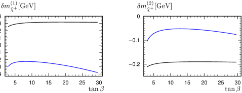
Fig. 6 shows the chargino pole masses at SPS1a’ as functions of . At the SPS1a’ value we find an absolute two-loop correction which is in the order of magnitude of the expected experimental uncertainty for this particle, see Table 1. Therefore, the inclusion of these corrections is mandatory when extracting -parameters from experiment.
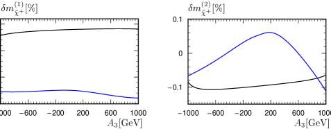
For Fig. 7 we set the third generation trilinear breaking parameters equal, . This parameter effects the mixing in the squark sector and therefore enters all the two-loop diagrams through the couplings and the sfermion masses.
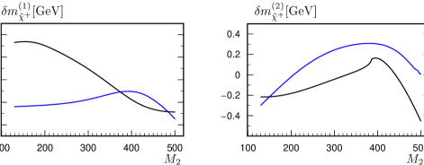
In Fig. 8 we assume gauge unification, . The plot is over , all other values are taken from SPS1a’.
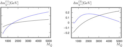
In Fig. 9 we show the one- and two-loop chargino mass shifts as a function of the third generation soft SUSY breaking masses . Again, all other parameters are taken from SPS1a’.
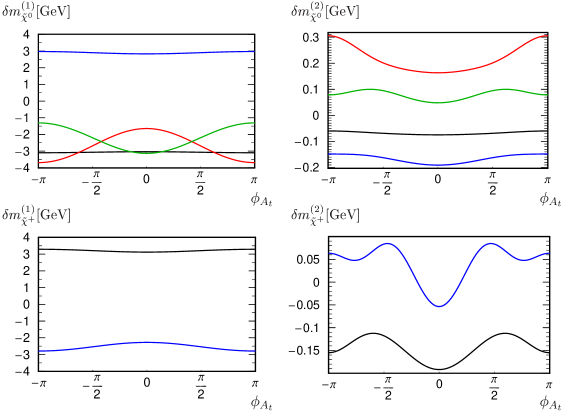
Finally, in Fig. 10 we investigate the dependence on , the complex phase of the soft trilinear breaking parameter . Extending previous work [14] we here include the neutralinos by taking complex. In the first column there are the one-loop corrections to the chargino and the neutralino pole masses and in the second the respective two-loop corrections. It can be seen that the influence of the phase is quite substantial at the two-loop level.
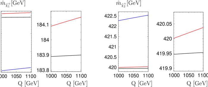
Fig. 11 shows the decrease of the scale dependence when the loop-level of the corrections is increased. The plots with one- (red) and two-loop (black) masses are zooms of the plots to their left where the running tree-level mass is included. The scale dependence is reduced considerably when going from the one- to the two-loop level. The remaining scaling comes from the uncancelled RGEs.
4 Conclusions
We have calculated the chargino pole masses in the MSSM to order and performed a detailed numerical study. The typical size of the two-loop corrections is comparable to the expected eperimental accuracy at future linear colliders and therefore needs to be taken into account when analyzing precision experiments. Our analytic expressions agree with previous generic results [7] and have been checked thoroughly. Extending previous work [14] we also include complex parameters in the neutralino case. Finally, we wrote a program [18] for this calculation with an interface to the commonly used SUSY Les Houches accord [19].
Appendix A Polxino: Short description of the program
Polxino [18] is a C-program for the evaluation of the pole masses of neutralinos and charginos in the MSSM. Up to now it contains the full one-loop level and all SQCD effects at the two-loop level. It makes considerable use of the TSIL program [23] and uses some of the generic functions of [25]. For convenience we provide a SLHA-interface [19]. We have carefully checked Polxino against the calculation described in this paper and in [14].
| MSSM_DATA member | description |
|---|---|
| gs, g1, g2 | gauge coupling constants |
| mue | -parameter |
| TB | |
| VEV | the square root of the sum of squared Higgs VEVs |
| MA02 | squared mass of |
| MQU[3], MQD[3], MLE[3] | quark and lepton-masses |
| M1, M2, M3 | gaugino masses |
|
MSL[3], MSE[3], MSQ[3],
MSU[3], MSD[3] |
bilinear soft susy breaking parameters |
| Af[4][3] | trilinear soft susy breaking parameters |
The source code contains the main file main.c which itself contains the code for a generic case, the evaluation of aforementioned pole masses
at the SPS1a’ benchmark point. Since the program currently uses long double (POL_REAL) and long double complex
(POL_COMPLEX) it is recommended that TSIL is compiled with the compiler flag
-DTSIL_SIZE_LONG
The central data struct in Polxino is
MSSM_DATA
which contains the whole set of MSSM parameters.
The subroutine loadSPC fills this struct from an SLHA-file and returns 1 if successful.
loadSPC(”SPheno.spc”,MSSM_DATA*);
The file SPheno.spc used by the main program was created by SPheno [26] and comes with Polxino.
If the content of the struct MSSM_DATA is to be changed after the file was loaded it must be kept in mind that
some of the information stored in the struct is derived from a smaller set of basic elements.
The basic parameters which may be subject to change are given in Table 2 with their respective index ranges in C/C++-notation.
The first index of Af labels the
type of the trilinear breaking parameter according to FeynArts. Af[0] denotes the neutrino case and should therefore be kept zero.
Af[1], Af[2] and Af[3] are the leptonic, up- and down-type set of parameters. All other indices of
the form [3] label the generation.
Calling
mssm_digest(MSSM_DATA*);
recalculates all the derived parameters in the struct from the basic ones and re-diagonalizes the mixing systems. Thus, it is
fairly simple to loop over a parameter that enters in many different places, e.g. the -parameter. The math used for this
re-diagonalization was extracted from some Fortran subroutines of LoopTools [27] and rewritten in the C-language.
The command
mssm_print(MSSM_DATA);
prints out all the information stored in the struct. Finally,
getneupole(int i, MSSM_DATA,
POL_REAL* Mpole1, POL_REAL* Gamma1,
POL_REAL* Mpole2, POL_REAL* Gamma2);
getchpole(int i, MSSM_DATA,
POL_REAL* Mpole1, POL_REAL* Gamma1,
POL_REAL* Mpole2, POL_REAL* Gamma2);
calculate the one- and two-loop pole masses of chargino (neutralino) and store the one- respectivly two-loop results in the
variables Mpole1 resp.Mpole2. The tree-level and one-loop widths are stored in Gamma1 and Gamma2,
respectively.
Acknowledgements
The authors would like to thank W. Majerotto, K. Kovařík and
C. Weber for discussion and many useful comments throughout the last year.
They especially thank W. Majerotto for his help in finalizing this work.
The authors acknowledge support from EU under the MRTN-CT-2006-035505
network programme. This work is supported by the ”Fonds zur Förderung
der wissenschaftlichen Forschung” of Austria, project No. P18959-N16.
References
- [1] G. Weiglein et al. [LHC/LC Study Group], Phys. Rept. 426 (2006) 47 [hep-ph/0410364].
- [2] TESLA Technical Design Report, Part III, Eds.: R. D. Heuer, D. Miller, F. Richard, and P. M. Zerwas, DESY 2001-011.
- [3] C. Adolphsen, et al., International Study Group Collaboration, International study group progress report on linear collider development, SLAC-R-559 and KEK-REPORT-2000-7.
- [4] A. Bednyakov, A. Onishchenko, V. Velizhanin and O. Veretin, Eur. Phys. J. C 29, 87 (2003) [hep-ph/0210258].
- [5] A. Bednyakov and A. Sheplyakov, Phys. Lett. B 604, 91 (2004) [hep-ph/0410128].
- [6] A. Bednyakov, D. I. Kazakov and A. Sheplyakov, hep-ph/0507139.
- [7] S. P. Martin, Phys. Rev. D 72 (2005) 096008 [hep-ph/0509115].
- [8] Y. Yamada, Nucl. Phys. Proc. Suppl. 157 (2006) 167 [hep-ph/0601263].
- [9] S. Heinemeyer, W. Hollik, H. Rzehak and G. Weiglein, AIP Conf. Proc. 903 (2007) 149.
- [10] M. Frank, T. Hahn, S. Heinemeyer, W. Hollik, H. Rzehak and G. Weiglein, JHEP 0702 (2007) 047 [arXiv:hep-ph/0611326].
- [11] G. Degrassi, S. Heinemeyer, W. Hollik, P. Slavich and G. Weiglein, Eur. Phys. J. C 28 (2003) 133 [arXiv:hep-ph/0212020].
- [12] S. Heinemeyer, W. Hollik and G. Weiglein, Eur. Phys. J. C 9 (1999) 343 [arXiv:hep-ph/9812472].
- [13] S. Heinemeyer, W. Hollik and G. Weiglein, Comput. Phys. Commun. 124 (2000) 76 [arXiv:hep-ph/9812320].
- [14] R. Schofbeck and H. Eberl, arXiv:hep-ph/0612276.
-
[15]
T. Hahn, Comput. Phys. Commun. 140 (2001)
418;
T. Hahn, C. Schappacher, Comput. Phys. Commun. 143 (2002) 54. - [16] J. Küblbeck, M. Böhm, A. Denner, Comput. Phys. Commun. 64 (1991) 345.
- [17] R. Mertig and R. Scharf, Comput. Phys. Commun. 111 (1998) 265 [hep-ph/9801383].
- [18] R. Schofbeck and H. Eberl, http://wwwhephy.oeaw.ac.at/tools/
- [19] P. Skands et al., JHEP 0407 (2004) 036 [arXiv:hep-ph/0311123].
- [20] W. Öller, H. Eberl, W. Majerotto and C. Weber, Eur. Phys. J. C 29 (2003) 563 [hep-ph/0304006].
- [21] T. Fritzsche , Eur. Phys. J. C 24 (2002) 619 [hep-ph/0203159].
- [22] S. P. Martin, Phys. Rev. D 65 (2002) 116003 [hep-ph/0111209].
- [23] S. P. Martin and D. G. Robertson, Comput. Phys. Commun. 174 (2006) 133 [hep-ph/0501132].
- [24] J. A. Aguilar-Saavedra et al., Eur. Phys. J. C 46 (2006) 43 [hep-ph/0511344].
- [25] S. P. Martin, http://zippy.physics.niu.edu/gluinopole/
- [26] W. Porod, Comput. Phys. Commun. 153 (2003) 275 [hep-ph/0301101].
- [27] T. Hahn and M. Perez-Victoria, Comput. Phys. Commun. 118 (1999) 153 [arXiv:hep-ph/9807565].