Luminous Red Galaxy Population in Clusters at $0.2\leq z\leq 0.6$

Abstract

We investigate statistical properties of LRGs in a sample of X-ray selected galaxy clusters at intermediate redshift ($0.2\leq z\leq 0.6$). The LRGs are selected based on carefully designed color criteria, and the cluster membership is assessed via photometric redshifts. As clusters and LRGs are both viewed as promising tracer of the underlying dark matter distribution, understanding the distribution of LRGs within clusters is an important issue. Our main findings include:

1. The halo occupation distribution of LRGs inside our cluster sample is $N(M)=k\times(M/10^{14})^{a}$ where $a=0.620\pm 0.105$ and $k=1.425\pm 0.285$ assuming a Poisson distribution for $N(M)$.

2. The halo occupation distribution of LRGs ($N(M)$) and the satellite distribution of LRGs ($N-1(M)$) are both consistent with being Poisson. To be more quantitative, we find $Var(N)/\langle N\rangle=1.428\pm 0.351$ and $Var(N-1)/\langle N-1\rangle=1.823\pm 0.496$.

3. The radial profile of LRGs within clusters when fitted with a NFW profile gives a concentration of $17.5^{+7.1}_{-4.3}$ ($6.0^{+3.2}_{-1.9}$) including (excluding) BLRGs (Brightest LRGs).

We also discuss the implications of these observations on the evolution of massive galaxies in clusters.

1 Introduction

The recent advent of large-scale galaxy surveys have revolutionized the field of observational cosmology. Deep spectroscopic surveys allows us to witness the young Universe when the building blocks of present-day galaxies are forming, and some of the well-known properties of the local galaxy populations are about to realize. The enormous amount of data gathered by wide area surveys produce galaxy samples with exquisite statistical precision, which makes it possible to single out the most fundamental properties that govern the physics of galaxy formation from the medley of observables.

Equally impressive has been the progress in the theoretical understanding of the structure formation in the Universe. Techniques such as direct numerical simulations and semi-analytic models can now reproduce the observed properties of galaxies, such as the luminosity function and 2-point correlation function, color, mass-to-light ratios over large ranges of environments and cosmic epochs (Kauffmann et al., 1999a, b; Springel et al., 2001; Cole et al., 2000; White & Rees, 1978).

Yet another approach, the so-called halo model, which is phenomenological in nature, has enjoyed popularity over the recent years. An essential ingredient of this method is the halo occupation distribution (HOD), which refers to the way galaxies (or substructures of dark matter halos) “populate” dark matter halos. In general, an HOD description includes the mean number of galaxies per halo $N$ as a function of halo mass, the probability distribution that a halo of mass $M$ contains $N$ galaxies $P(N|M)$, and the relative distribution (both spatial and velocity) of galaxies and dark matter within halos (Berlind & Weinberg, 2002).

The halo model formalism allows fast exploration of a wide range of HODs; an HOD that reproduces the observed clustering properties and luminosity function of galaxies can be further studied to reveal the physical processes that lead to galaxy formation and understanding of cosmological parameters. Examples of using halo model formalism to reproduce observables in order to reveal parameters in cosmology, galaxy evolution and formation includes (e.g. Abazajian et al., 2005; White et al., 2007; Yoo et al., 2006; Zheng & Weinberg, 2007; Kulkarni et al., 2007).

Despite the success in both observational and theoretical sides, there remains some unsolved problems regarding the formation of the massive, (usually) early type, galaxies. These galaxies appear ” red and dead”, with the majority of the stars forming at high redshift ($z>\sim 2$) and evolving passively since. Within the cold dark matter (CDM) paradigm, in which massive galaxies are built by smaller galaxies via mergers in the late times, mergers between gas poor systems (“dry” mergers) seem to be a promising route to form giant galaxies. Observationally, however, the overall importance of dry mergers is still under heated debate.

Luminous Red Galaxies (LRGs) are massive galaxies composed mainly of old stars, with little or no on-going star formation. They demonstrate very consistent spectral energy distribution (SED). Their SEDs mainly consist of old star spectrum, most notably for the $4000$Å break. This allows one to photometrically determine their redshifts fairly accurately (see Padmanabhan et al., 2005). With the accurate photometric redshifts of LRGs, one can probe a larger volume of the universe, thus giving better constraints on the formation of massive galaxies. By studying the HOD of the LRGs, we aim to provide a simple quantitative description of these galaxies in massive dark matter halos, which will enable direct comparison with predictions of galaxy formation models.

Here we aim to provide observational constraints on the HOD of the LRGs based on a sample of 47 intermediate-redshift clusters from the ROSAT 400d survey (Burenin et al., 2006), with photometric data from the Sloan Digital Sky Survey (SDSS; Stoughton et al., 2002). Using X-ray properties of these clusters to define the cluster center and estimate the cluster binding mass, we determine the mean halo occupation number $N$ as a function of mass from $\sim 1\times 10^{14}M_{\odot}$ to $\sim 8\times 10^{14}M_{\odot}$ and also investigate the LRG distribution and luminosity distribution within the clusters.

In §2, we briefly describe the X-ray cluster catalog that we utilize and the construction of SDSS LRG sample. In §3, we present our method and findings on the LRG distributions within the clusters and the mean halo occupation number. We discuss what is a good mass tracers and evolution of massive galaxies in §5. Possible systematics that may affect our results are discussed in §4.

Throughout the paper we assume the cosmological parameters to be the WMAP values (Spergel et al., 2006): $\Omega_{m}h^{2}=0.1277$, $h=0.732$ and the Hubble parameter $H_{0}=73\,h_{73}$ km s^-1 Mpc^-1.

2 Data

2.1 Cluster Sample

Our cluster sample is drawn from the 400 square degree ROSAT PSPC Galaxy Cluster Survey (Burenin et al., 2006) (hereafter the 400d survey), which is an extension of the 160 square degree survey (Vikhlinin et al., 1998). The survey detects extended X-ray sources in archival ROSAT PSPC images down to a flux limit of $1.4\times 10^{-13}\,{\rm erg\,s}^{-1}{\rm cm}^{-2}$, with extensive optical spectroscopic follow up. Out of the 266 clusters detected in the survey, 47 lie within the redshift range $0.2\leq z\leq 0.6$ and are covered by SDSS DR5. The redshift range is chosen to be consistent with the photometric cuts designed to select a homogeneous LRG sample across a wide range in cosmic epochs.

The cluster catalog from the 400d survey provides estimates of cluster center, redshift, and X-ray luminosity $L_{X}$, which is used to estimate the cluster mass. Some of the basic information of the clusters in our sample is given in Table 1.

2.2 LRG Data from Sloan Digital Sky Survey

The Sloan Digital Sky Survey has taken $ugriz$ CCD images of $10^{4}$ deg² of the high-latitude sky. A dedicated 2.5m telescope at Apache Point Observatory images the sky in 5 bands between 3000Å  and 10000Å (Fukugita et al., 1996) using a drift-scanning, mosaic CCD camera (Gunn et al, 1998; Gunn et al., 2006), detecting objects to a flux limit of $r\sim 22.5$ mag. The survey selects $10^{6}$ targets for spectroscopy, most of them galaxies with $r<17.77$ mag (Gunn et al, 1998; York, Adelman, Anderson, Anderson, et al., 2000; Stoughton et al., 2002). This spectroscopic follow-up uses two digital spectrographs on the same telescope as the imaging camera. Details of the galaxy survey are described in the galaxy target selection papers (Eisenstein et al., 2001; Strauss et al., 2002); other aspects of the survey are mainly described in the Early Data Release paper (Stoughton et al., 2002). All the data processing, including astrometry (Pier et al., 2003), source identification and photometry (Lupton et al., 2001; Hogg et al., 2001; Ivezic et al., 2004), calibration (Fukugita et al., 1996; Smith et al., 2002), spectroscopic target selection (Eisenstein et al., 2001; Strauss et al., 2002; Richards et al., 2002), and spectroscopic fiber placement (Blanton et al., 2003) are done automatically via SDSS software (Tucker, et al., 2006). The SDSS is well-underway, and has had six major releases (Adelman-McCarthy et al., 2007).

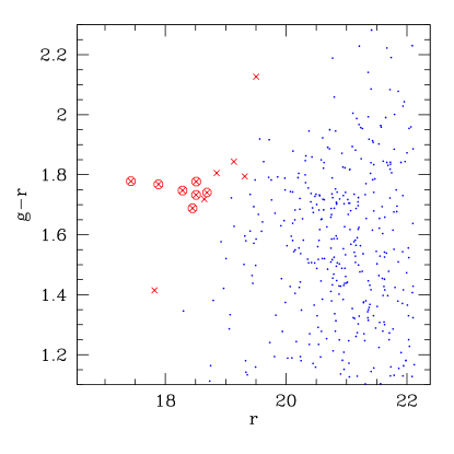
We utilize the photometric LRGs from SDSS constructed as described in Padmanabhan et al. (2005, hereafter P05). The LRGs have been very useful as a cosmological probe since they are typically the most luminous galaxies in the universe, thus they probe a larger volume than most other tracers. On top of this, they also have very regular spectral energy distributions and a prominent 4000Å break, making photometric redshift estimation much easier than the other galaxies. We plot the color magnitude diagram for one of the cluster and show that the LRGs in the cluster are the bright red galaxies that follow nicely along the red sequence (see Fig 1).

Figure 1: Color-magnitude diagram of objects toward the field of Cluster 142. Those satisfying cuts I and II (see Eqn. 2 and 3) are shown as crosses and squares respectively. The red circles are selected LRGs and the blue dots are objects detected in SDSS photometrically. As shown, the selected LRGs lie very systematically along the red sequence of the cluster.

Our selection criteria are based on the spectroscopic selection of LRGs described in Eisenstein et al. (2001), extended to lower apparent luminosities (P05). We select LRGs by choosing galaxies that both have colors consistent with an old stellar population, as well as absolute luminosities greater than a chosen threshold. The first criterion is simple to implement since the uniform SEDs of LRGs imply that they lie on an extremely tight locus in the space of galaxy colors; we simply select all galaxies that lie close to that locus. More specifically, we can define three (not independent) colors that describe this locus,

$$c_{\perp} \equiv (r-i)-0.25(g-r)-0.18\,\,\,,$$

$$d_{\perp} \equiv (r-i)-0.125(g-r)\,\,\,,$$

$$c_{||} \equiv 0.7(g-r)+1.2(r-i-0.18)\,\,\,,$$ (1)

where $g$, $r$, and $i$ are the SDSS model magnitudes in these bands respectively. We now make the following color selections,

$${\rm Cut\,\,I:} \mid c_{\perp}\mid<0.2;$$

$${\rm Cut\,\,II:} d_{\perp}>0.55,\,\,\,g-r>1.4,$$ (2)

as well as the magnitude cuts

$${\rm Cut\,\,I:} r_{Petro}<13.6+c_{||}/0.3;$$

$$r_{Petro}<19.7;$$

$${\rm Cut\,\,II:} i<18.3+2d_{\perp},$$ (3)

$$i<20.$$

Making two cuts (Cut I and Cut II) is convenient since the LRG color locus changes direction sharply as the 4000Å break redshifts from the $g$ to the $r$ band; this division divides the sample into low redshift (Cut I, $z<0.4$) and high redshift (Cut II, $z>0.4$) samples. More details of these color selection criteria are thoroughly described in P05.

We do however apply slightly different cuts than those adopted in P05: we limit our samples to sky regions where

$$E(B-V)\leq 0.08$$ (4)

and data taken under seeing condition of

$$FWHM<2.0^{\prime\prime}.$$ (5)

These cuts in extinction and seeing are applied simply by excluding areas at which the galaxy overdensity drops significantly. Furthermore, there are a few regions in SDSS that have 60% more red objects and less blue objects; we decide to throw away these regions.

We slice our LRG sample into two redshift bins: $0.2\leq z_{photo}\leq 0.4$ and $0.4\leq z_{photo}\leq 0.6$. We also regularized our redshift distribution as described in P05. For our sample, we have 855534 galaxies, covering 2,025,731 resolution 10 HEALpix pixels, each with area of $11.8$ $\rm{arcmin}^{2}$, giving 0.422334 gal/pix.

We then estimate the photometric redshift of these LRGs with the algorithm developed by P05. The typical uncertainty of the photo-$z$’s is $\delta_{z}=\sigma_{z}/(1+z)\approx 0.03$ (see P05).

3 Analysis

3.1 Method

We estimate the cluster virial mass $M_{200}\equiv(4\pi/3)r_{200}^{3}\times 200\rho_{c}$ from the X-ray luminosity using the mass–luminosity relation given by Reiprich & Böhringer (2002)

$$\log\left[{1.4^{2}L_{X}(0.1-2.4{\rm\ keV})\over h_{73}^{-2}10^{40}\,{\rm erg\ s}^{-1}}\right]=A+\alpha\log\left({1.4M_{200}\over h_{73}^{-1}M_{\odot}}\right),$$ (6)

where $A=-20.055$ and $\alpha=1.652$. The radius $r_{200}$ is defined such that the enclosed mean overdensity is 200 times the critical density $\rho_{c}$. The corresponding angular extent is $\theta_{200}$. The mass–luminosity scaling relation provides a mass estimate accurate to $<50\%$ (Reiprich & Böhringer, 2002) and a virial radius $r_{200}$ estimate accurate to 15%.

As we now have the redshifts and positions of these clusters, we locate the LRGs as described in §2.2 in each of these clusters. We look for LRGs that are within a cylinder of radius $\theta_{200}$ and length of $\Delta_{z}=0.06$ from the cluster center in both position and redshift space (i.e. $z_{LRG}=z_{c}\pm 0.03$). We choose $\delta_{z}=0.03$ since that is the typical $1\sigma$ error on the LRG photometric redshift (P05) and $z_{c}$ is the cluster redshift. More discussion on the choice of cluster radius and $\delta_{z}$ will be described in §4.

Since we are relying on the photometric redshifts of the LRGs to find out whether a LRG sits in certain cluster or not, we take into account the effects of the following mechanisms that may lead to over-(or under-)estimate of the number of LRGs in each cluster:

i. LRG identification failure: There is an identification failure rate of $\sim 1\%$ (Padmanabhan et al., 2006). This is the rate of which a LRG (photometrically chosen) is actually a star or a quasar after we get the spectra of the object.

ii. Interlopers: There is a finite probability of finding LRGs inside the cluster purely by chance, we call these interlopers. We access the expected number of interlopers in each cluster by looking at the average number of LRGs in sky (2D projected) in the solid angle of radius = $\theta_{200}$ of the cluster and the average probability of finding a LRG in redshift range of $z_{c}\pm\delta_{z}$ where $\delta_{z}=0.03$ (as defined above). We can write down the expected number of interlopers ($\langle N_{int}\rangle$) as:

$$\langle N_{int}\rangle=\bar{n}\pi\theta^{2}\int_{z_{c}-\delta_{z}}^{z_{c}+\delta_{z}}P(z_{p})dz_{p}$$ (7)

where $P(z_{p})$ is the normalized (photometric) redshift distribution of LRGs, $\bar{n}$ is the 2D average LRG density.

iii. Missing galaxies due to errors in photometric redshift: As an LRG can be scattered out of the cluster (due to photoz error), we need to account for this process by looking at the probability of LRG having been photometrically determined to be outside of the cluster, but in fact has spectroscopic redshift that falls within the range of the cluster:

$$P(|z_{p}-z_{c}|>\delta_{z},||z_{s}-z_{c}|<\delta_{z})=\int_{z_{min}}^{z_{max}}(F(z_{s})+B(z_{s}))dz_{s}\,\,\,,\\$$ (8)

$$z_{min}=max(0.05,z_{c}-\delta_{z_{c},in})\,\,\,,$$

$$z_{max}=min(0.7,z_{c}+\delta_{z_{s},in})\,\,\,,$$

$$F(z)=\int_{-\infty}^{z_{c}-\delta_{z}-z}P(\delta,z)d\delta\,\,\,,$$

$$B(z)=\int_{z_{c}+\delta_{z}-z}^{+\infty}P(\delta,z)d\delta\,\,\,,$$ (9)

where $P(\delta,z)$ is the probability of finding $\delta$ ($=z_{s}-z_{p}$) at $z_{s}$, given by Padmanabhan et al. (2005) and these are only characterized within the spectroscopic redshift range from $z=0.05$ to $z=0.7$. $\delta_{z_{c},in}$ is the redshift range we allow a LRG to be a cluster member when we have its spectroscopic redshift, and this is set to be $0.01$.

We then calculated the corrected LRG counts in each cluster via the following:

$$\langle N_{corr}\rangle=(\langle N_{obs}\rangle-\langle N_{int}\rangle)/f(z_{p},z_{c},z_{s})\,\,\,,\\$$ (10)

$$f(z_{p},z_{c},z_{s})=(1-P(|z_{p}-z_{c}|>\delta_{z}||z_{s}-z_{c}|<\delta_{z}))\times(1+F))\,\,\,,$$ (11)

and $F$ is the LRG identification failure rate.

We list these corrected LRG counts in Table 1.

To convert the observed magnitudes of the LRGs into the rest-frame luminosity at $z=0$, we follow the evolution of a simple stellar population formed in a burst at $z=5$, with solar metallicity and Salpeter initial mass function, using the model of Bruzual & Charlot (2003). The LRGs are selected so that their present-day magnitude lies in the range $-23.5\leq M_{g}\leq-21$ (roughly corresponding to $1$–$7L_{*}$, where $L_{*}$ is the characteristic luminosity).

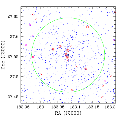
For each cluster, we visually inspect the spatial and color distributions of LRGs with respect to all objects detected by SDSS. An example is shown for cluster 142. Perhaps not surprisingly, the spatial distribution of the LRGs seems concentrated towards cluster center (Fig. 2).

Figure 2: Spatial distribution of LRGs in Cluster 142. The blue points represent all objects detected in the SDSS photometric survey. Those satisfying cuts I and II are shown as crosses and squares, respectively. The LRGs that have photo-$z$ consistent with the cluster redshift ($z=0.353$) are represented as circles. The black cross denotes the centroid position of the ICM. The green circle is the region encircled by the virial radius of the cluster.

A general scenario that has been painted about LRGs and clusters is that there is a massive red galaxy sitting right in the middle of the cluster. Then some other process may sometimes bring in other massive red galaxies, but they will probably sink into the center over several dynamical times.

Here, we actually have the ability to see if this scenario is true: we have the number of LRGs inside each of these clusters and we know where they are. Below we present results on the spatial distribution of LRGs in clusters (§3.2) and the halo occupation number (§3.3). and the LRG multiplicity function (§3.5),

3.2 Spatial Distribution of LRGs within Clusters

Figure 3: The distribution of LRGs in the clusters. The number of LRGs in each bin are normalized by dividing the number of LRGs in each bin by the total number of LRGs in all bins.

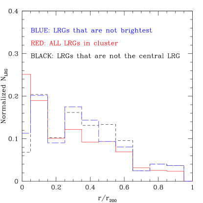
We show the spatial distribution of LRGs within the clusters in Fig. 3. Previous studies (e.g. Jones & Forman, 1984; Lin & Mohr, 2004) have shown that brightest galaxies tend to lie at the center of the clusters. Here we test if this is true for the LRGs. We plot the distribution of brightest LRGs in each of the cluster alongside with their companions in each of the cluster (see Fig. 4). One realizes that most ($\sim 80\%$) of the brightest LRGs resides within the inner 20% of the scaled radius of the cluster. Therefore, we are consistent with the picture of having brightest galaxies lying at the centers of clusters. However, there is a significant fraction of clusters that does not follow this rule.

Figure 4: (Above) The distribution of brightest LRGs (BLRGs) and the non-brightest LRGs in the clusters. As shown above, the BLRGs tend to lie at centers of the clusters, while the ones that are not BLRGs have a shallower radial distribution. (Below) The distribution of most central LRGs and the non-central LRGs in the clusters. The distribution of the central LRGs are very similar to the BLRGs.

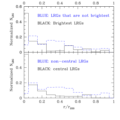
The question of whether the centers of intracluster gas coincide with the central LRGs (defined as the LRG closest to the centroid of the X-ray emitting gas) is also very important to the understanding of the formation of galaxies. We investigated the distribution of the central LRGs inside the cluster (see Fig. 4). There are $\sim 20\%$ of the “central” LRGs which are not central at all. This may suggest a few scenarios, one being that the cluster is not relaxed enough for the central LRG to sit at the center of the gravitational potential (which is supposedly traced by the intracluster light). The centroiding of the clusters in X-ray is called into question, and we will address this in §4.

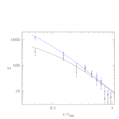
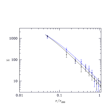
The profile of galaxies in cluster is a key ingredient to the halo model formalism. One would like to understand how statistically LRGs populate the clusters they are residing. We try to fit the NFW profile here to the LRG surface density of stacked clusters in our sample and find that the concentration of the surface density to be $17.5^{+7.1}_{-4.3}$ with $\chi^{2}=4.29$. We also plot the fitted profile in Fig. 5. We also fit the NFW profile to LRG surface density of stacked clusters without the BLRG (Brightest LRG in the cluster), and this gives a concentration of $6.0^{+3.2}_{-1.9}$ with $\chi^{2}=6.6$. Both profiles have very similar concentration as the K-band cluster profile discussed in Lin & Mohr (2007) (see Figure 6). Errors in $r_{200}$ determination do not affect the fit in any significant fashion as demonstrated in Lin & Mohr (2007) appendix .

Figure 5: The distribution of LRGs in the clusters with the fit to the NFW profile. Blue line: we fit the surface density of the LRGs (including BLRGs) to a NFW profile and get a concentration of $17.5^{+7.1}_{-4.3}$ with $\chi^{2}=4.29$. Black line: we fit the surface density of the LRGs (excluding BLRGs) to a NFW profile and get a concentration of $6.0^{+3.2}_{-1.9}$ with $\chi^{2}=6.6$.

Figure 6: The distribution of LRGs in the clusters with the fit to the NFW profile. Blue line: we fit the surface density of the LRGs (including Brightest LRGs) to a NFW profile and get a concentration of $17.5^{+7.1}_{-4.3}$ with $\chi^{2}=4.29$. Black line shows the fit of the profile of bright galaxies (normalized to this plot) from (Lin et al., 2006).

3.3 Halo Occupation Number

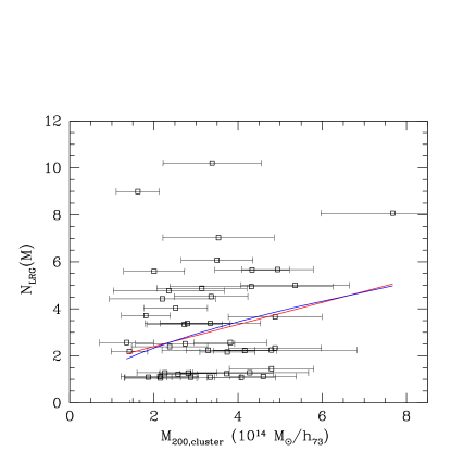
As the halo occupation number of the clusters is a key ingredient to the halo model formalism, we investigate the number of LRGs in these clusters as a function of their masses. As the size of our sample is not large and the mass estimate o the clusters are accurate to $30\%-50\%$ only, one will have to be extra cautious in finding a fit for the average number of LRGs in the mass range of these clusters. We take the following approach, assuming two different models:

$$N(M_{t})=a\times M_{t}+k$$

$$N(M_{t})=k\times M_{t}^{a}$$

where $M_{t}$ is true value of cluster virial mass in $10^{14}h_{73}^{-1}M_{\odot}$, a Poisson distribution of $N(M_{t})$ and two distributions for the probability finding $M_{t}$ given $M_{i}$ where $M_{i}$ is the measured mass of the i-th cluster (in same units as in $M_{t}$), one being Gaussian, the other Log-Normal. In short, we have the following:

$$L_{tot}=\prod_{i}^{N_{c}}\int{P(N_{i},M_{t,i}|a,k)P(M_{t,i}|M_{i})}dM_{t,i}$$

$$\log P(N,M|a,k)=N\times\log(\mu)+const-\mu$$

$$\log P_{g}(M_{t}|M_{i})=-(M_{t}-M_{i})^{2}/(2\sigma_{M}^{2})+const$$

$$\log P_{ln}(M_{t}|M_{i})=-(M_{t,l}-M_{i,l})^{2}/(2(\sigma_{M_{l}})^{2})+const$$

(13)

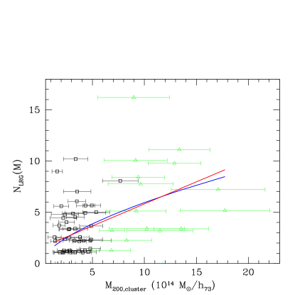
where $\mu=a\times M+k$ or $\mu=k\times M^{a}$, $M_{t,i}$ stands for the $M_{t}$ for the i-th cluster and $M_{x,l}$ stands for $\log_{10}(M_{x})$ for the above mentioned form of fit. We then maximize the total Likelihood within a grid of resolution $100,1000,10000$ for both $a$, $k$ and we also vary the size of $dM_{t,i}$ to ensure that our results are robust with respect to varying grid size. We also try a variety of ranges for both $a$ and $k$ (such as $0<a<20$, $-10<a<10$ and $0<a<3$; and $0<k<20$, $-20<k<20$ and $0<k<5$), and make sure we get the same answer. This linear fit with $P_{g}(M_{t}|M_{i})$ gives $a=0.455\pm 0.215$ and $k=1.605\pm 0.705$ for $68.3\%$ confidence intervals. This power-law fit with $P_{g}(M_{t}|M_{i})$ gives $a=0.515\pm 0.245$ and $k=1.725\pm 0.540$ for $68.3\%$ confidence intervals. See Fig. 7 for the data and the fit using $P_{ln}(M_{t}|M_{i})$.

Figure 7: The number of LRG per halo $N$ as a function of binned halo mass ($10^{14}h_{73}^{-1}M_{\odot}$), the fit (red line) is calculated by maximizing the likelihood given a model of $N(M_{t})=a*M_{t}+k$ where $M_{t}$ is the true measure of $M_{200}$ in $10^{14}h_{73}^{-1}M_{\odot}$, assuming Poisson distribution of $N(M_{t})$, where $M_{t}$ is the true mass of the cluster. We also assume a log-normal distribution for probability of $P_{ln}(M_{t}|M_{i})$, where $M_{i}$ is the measured mass. This gives $a=0.470\pm 0.205$ and $k=1.455\pm 0.72$. The blue line fit is calculated by maximizing the likelihood given a model of $N(M_{t})=k*M_{t}^{a}$ and it gives $a=0.560\pm 0.250$ and $k=1.575\pm 0.525$.

3.4 $N(M)$ distribituion: Poisson or not?

Since we assume a Poisson distribution for $N(M_{t})$ (hereafter $N$ for simplicity in this section), we test if this is a good assumption by looking at $(\langle N^{2}\rangle-\langle N\rangle^{2})/\langle N\rangle$. We define $\gamma_{N}=(\langle N^{2}\rangle-\langle N\rangle^{2})/\langle N\rangle$, and since we only have $N(M_{i})$, but not $N$ (Number of LRG given the true measure of cluster mass) for each cluster, therefore, we have to consider the contribution of scatter from the various systematic effects we mentioned in §3.1:

$$\langle N_{i}^{2}\rangle_{(M_{i})}=\langle N_{int}\rangle^{2}+\langle N_{int}\rangle+Y+Z+W$$

$$Y=2f\langle N_{int}\rangle\langle N\rangle_{(M_{i})}$$

$$Z=\int dM_{t}[P(M_{t}|M_{i})(\langle N\rangle^{2}_{(M_{t})}+V)$$

$$V=\gamma\langle N\rangle_{(M_{t})}$$

$$W=f(1-f)\langle N\rangle_{(M_{i})}$$ (14)

where $f=f(z_{p},z_{c},z_{s})$ and is defined in §3.1, $N_{int}$ is the number of interloper as discussed in §3.1 and $X_{(M_{i})}$ ($X_{(M_{t})}$) means the quantity X conditioned on $M_{i}$ ($M_{t}$).

Subtracting $\langle N(M_{i})\rangle^{2}_{(M_{i})}$ from the equation will reduce to:

$$\langle N_{i}^{2}\rangle_{(M_{i})}-\langle N(M_{i})\rangle^{2}_{(M_{i})}=PQ+R+S+T$$

$$P=f^{2}\gamma+f(1-f)$$

$$Q=\langle N\rangle_{(M_{i})}$$

$$R=\langle N_{int}\rangle$$

$$S=f^{2}(\int dM_{t}([P(M_{t}|M_{i})\langle N\rangle^{2}_{(M_{t})})$$

$$T=-f^{2}\langle N\rangle^{2}_{(M_{i})}$$ (15)

Note that $\langle N\rangle_{(M_{i})}$ = $\int dM_{t}[P(M_{t}|M_{i})\langle N\rangle_{(M_{t})}]$.

Figure 8: To test whether our assumption of a Poisson distribution for $N(M_{t})$ is valid, we compute $\langle N(N-1)\rangle/\langle N\rangle^{2}$ for the combined sample of $400d+Yx$. It does not deviate drastically from being Poisson.

A Poisson distribution is completely characterized by its first moment, $\gamma$ would be 1 if the distribution is completely Poisson. We calculate the $\gamma$ from the combined sample of $400d$ and $Yx$ (please refer to §4 for a description of $Yx$ sample) sample and use $\langle N\rangle$ from the fit of $N(M)=k\times(M/10^{14})^{a}$. We bin the cluster such that there are equal number of clusters in each mass bin (See Figure 8). We find that $\gamma=1.428\pm 0.351$ and thus the $N(M_{t})$ distribution is consistent with being Poisson.

Furthermore, one important ingredient of halo occupation distribution is the assumption of Poisson distribution of the satellite galaxies. We test the assumption here by computing $(\langle(N-1)^{2}\rangle-\langle(N-1)\rangle^{2})/\langle(N-1)\rangle$ for the $\langle N-1\rangle$ distribution (see Fig. 9) in a similar way as we compute $\gamma$ for the $\langle N\rangle$ distribution. We find that $\gamma_{N-1}=1.823\pm 0.496$ and so the satellite LRG distribution in clusters is also consistent with being Poisson. However, one should note that it is mathematically impossible for both $N$ and $N-1$ to be both exactly Poisson for the same distribution. The errorbars are calculated via $\sigma(X)=\sqrt{(}(X-\bar{X})^{2})/N_{c}$.

Figure 9: To test if the satellite LRG distribution is Poisson, we calculate $(\langle(N-1)^{2}\rangle-\langle(N-1)\rangle^{2})/\langle(N-1)\rangle$ for the combined sample of $400d+Yx$. It is consistent with being Poisson.

3.5 LRG Multiplicity Function

Finally we study the multiplicity of LRGs in clusters (Fig. 10).

Figure 10: The volume weighted multiplicity function of LRGs in these clusters. Blue (Black) line: the volume weighted multiplicity function for clusters with X-ray luminosities $>=$ ($<$) $10^{44}ergs^{-1}$. The variance is calculated by taking the sum of $1/(V_{max}^{2})$ for each $N_{LRG}$ bin.

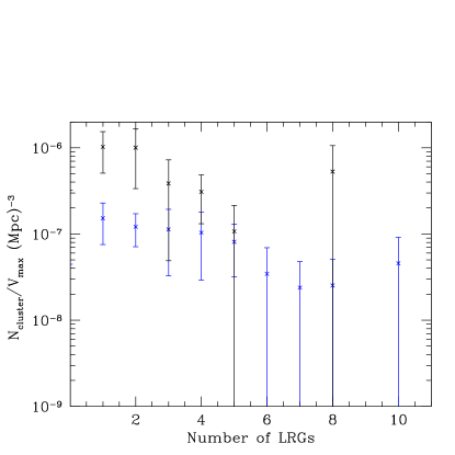
We calculate the multiplicity function by counting the $1/V_{max}$ weighted number of cluster in each bin. We compute $V_{max}$ (the comoving search volume of the cluster) by:

i.We find the flux of the cluster via the following Burenin et al. (2006):

$$f=\frac{L}{4\pi d_{L}(z)^{2}}K(z)$$ (16)

where $L$ is the luminosity of the cluster, $d_{L}(z)$ is is the cosmological luminosity distance, $K(z)$ is the K-correction factor for X-ray clusters (for more details see Burenin et al. (2006)).

ii. We find the comoving search volume that each cluster with luminosity L can be detected given by the following:

$$V_{max}(L)=\int_{z=0}^{z=z_{c}}P_{sel}(f,z)\frac{dV}{dz}dz$$ (17)

where $P_{sel}(f,z)$ is the selection efficiency of the 400 square degrees ROSAT PSPC Galaxy Cluster Survey provided by A. Vikhlinin and R. Burenin (private communication), $dV/dz$ is the cosmological comoving volume per redshift interval (see Burenin et al. (2006) for more details).

4 Systematics

4.1 Uncertainties in the Choice of Cluster Radius

We choose to use $\theta_{200}$ since it is closest to the virial radius of the clusters. We also look at how the uncertainties of $r_{200}$ will affect our results. $r_{200}$ is accurate up to $\sim 10\%$ (Reiprich & Böhringer, 2002). We calculate the following to determine the effective number of LRGs we are missing due to uncertainties in $r_{200}$:

$$\int_{0}^{r_{200}}\rho(r)dr/\int_{0}^{1.1r_{200}}\rho(r)dr=0.95$$ (18)

and

$$\int_{0}^{r_{200}}\rho(r)dr/\int_{0}^{0.9r_{200}}\rho(r)dr=1.06$$ (19)

We set the density profile $\rho(r)$ as a NFW profile with concentration of 8 (which is approximately what we get when we fit the surface density of the cluster when we exclude the BCG). This shows that the uncertainties in $\theta_{200}$, thus $r_{200}$ only affect our estimation of $N(M)$ at the level of $\sim 5\%$.

4.2 Mass Estimation and Sample Selection

Cluster mass estimation is crucial in our analysis, as it defines the cluster virial region to search for member LRGs, and provides a fundamental radius to scale the distance of LRGs to cluster center. We infer cluster mass through the X-ray luminosity–mass scaling relation (Reiprich & Böhringer, 2002), which has been shown as a unbiased estimator (Reiprich, 2006). Compared to other X-ray–based cluster proxies such as temperature and $Y_{X}$ (the product of gas mass and temperature, which is proportional to the thermal energy of the cluster Kravtsov et al. 2006), $L_{X}$–$M$ correlation shows higher degree of scatter. We therefore seek for another cluster sample with better measured mass (despite without well-defined selection criteria).

Recently, Maughan et al. (2007) have presented a large cluster sample selected from the Chandra archive, for which the cluster mass is inferred from $Y_{X}$, and the cluster center is inferred from the Chandra images. 26 of these clusters lie within our SDSS DR5 masks and the redshift range $0.2\leq z\leq 0.6$. 16 of these 26 clusters do not overlap with our 400d sample and we use them to examine the results presented in §§3.2 & 3.3 (hereafter the $Y_{X}$ sample).

Figure 11: Distribution of the clusters on the mass–redshift plane. The squares, red points, and blue points denote the whole 400d survey sample, the subsample used in this study, and the $Y_{X}$ sample, respectively.

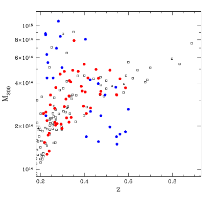
Because of the flux-limited nature of the 400d survey, low mass ($\sim 10^{14}M_{\odot}$) clusters will be only detected at lower redshifts. In Fig. 11 we show the mass distribution of the whole 400d sample (open squares) and the subsample used in our analysis (red points) within $0.2\leq z\leq 0.9$. It shows that our sample is a random subsample of the whole 400d sample Interestingly, at $z\sim 0.3$ the 400d survey clusters cover a larger range in mass than at other redshifts. It is also clear that the halo occupation numbers of clusters of lower masses in Fig. 7 would be biased to those at $z\leq 0.3$. In Fig. 11 we also show the distribution of the $Y_{X}$ sample. Very curiously, the distribution of this sample on the mass–redshift space seems to be roughly orthogonal to that of our 400d sample. Since our results derived from the $Y_{X}$ sample is consistent with those based on the 400d sample, we combine the two samples to enhance the mass coverage (especially for clusters at $z\geq 0.4$) and the statistical signal. We calculated the $N(M)$ for the combined sample and assuming power-law model, we have $N(M)=k*(M/10^{14})^{a}$, where $a=0.620\pm 0.105$ and $k=1.425\pm 0.285$, see Fig 12. A more detailed result table is shown at Table 2.

Figure 12: Combining the $Y_{X}$ sample (green triangles), we have a larger mass coverage, thus giving stronger constraints on the slope. We have fairly similar fits between the two different models (linear (red) and power-law (blue)). The fits are also consistent with the respective fits using only clusters from 400d survey.

5 Discussion and Summary

5.1 What is a good mass tracer?

As clusters are becoming more important cosmological tools, we need to characterize the masses of clusters more than ever. “What is a good mass tracer?” has been a very well-motivated question.

Here we try to investigate a few options that people have suggested before as possible solutions:

Fist, as we see earlier in §3.3, the mean number of LRGs does not trace the masses accurately.

We quantify this by looking at the scatter of the $N_{LRG}-M$ relation by the following quantities in a 3 mass bins:

$$\sigma(ln(N_{LRG}))=\frac{\sqrt{(}\gamma)}{\sqrt{(}N_{LRG})}$$

$$\sigma(ln(M))=\frac{1}{a}\sigma(ln(N_{LRG}))$$ (20)

where a is as defined in $N(M)=k\times(M/10^{14})^{a}$. We found that the scatter in $ln(N_{LRG})$ ($ln(M)$) in low, middle and high mass bins are $0.332$ ($0.535$) dex (at $M=2.22\times 10^{14}h_{73}^{-1}M_{\odot}$), $0.281$ ($0.452$) dex (at $M=3.81\times 10^{14}h_{73}^{-1}M_{\odot}$) and $0.21$ ($0.340$) dex (at $M=9.56\times 10^{14}h_{73}^{-1}M_{\odot}$) respectively.

Second, we look at the luminosities of the central LRG. As previous studies suggested in some bands, the brightest cluster galaxies traces the mass of the cluster (Lin & Mohr, 2004) and that the brightest cluster galaxies tend to be the central galaxies of the cluster, we look at the relation between the luminosities of the brightest LRG in clusters and their X-ray masses. However, the correlation between the distribution of luminosities of central LRG and the masses of the clusters in our sample does not look promising(see Fig. 13).

Figure 13: (Above) Luminosities of the central LRGs for each cluster. (Below) Luminosities of the brightest LRGs for each cluster.

We then look at the correlation between the luminosities of the brightest LRG and their cluster X-ray masses. However, it does not seem to be promising either (see Fig. 13). This is also seen in Lin & Mohr (2004) when we look at the same mass range and when one looks at the correlation between the brightest LRGs and the richness of the maxBCG catalog (Koester et al., 2007), there is not a strong correlation for 14,000 clusters (R. Reyes 2007, private communication). However, there are several caveats that would require further investigations, such as the possibility of photo-z failure for the CLRG or BLRG in the clusters and possible photometry problem that could destroy the correlation. We look into the available spectroscopic data in SDSS and found no extra LRGs that are targeted by the SDSS spectroscopy. This rules out the possible missing LRGs that have $M_{r}$ of range $\sim-20.8$ (at $z=0.2$) and $\sim-22.5$ (at $z=0.6$). Furthermore, as we investigated earlier, only 4 clusters do not have LRGs and we find $\sim 70\%$ of BLRGs lie in the central $\sim 20\%$ of the virial radius, thus, most clusters do have a LRG at their centers. If we are missing Brightest LRGs in centers of clusters, we need to expect the scenario of having more than 1 LRG at the central $\sim 20\%$ of cluster virial radius to be prevalent. This scenario is not supported by the distribution of LRGs as shown in Figure 4. Given the caveats and findings here, we conclude that further work will be needed to make this more quantitative, especially to quantify the effect of photometry errors on the correlation.

5.2 Evolution of Massive Galaxies

Insights into the evolution of massive galaxies in clusters may be gained by comparing some of the results presented in §3 with the properties of cluster galaxies in the local Universe. For consistency with our LRG selection, we select nearby cluster galaxies by the requirement that they are one magnitude more luminous than the characteristic magnitude ($M_{*}-1$).

We first examine the spatial distribution of massive galaxies within clusters. Lin & Mohr (2004), with a large sample of clusters at $z<0.2$, find that luminous cluster galaxies ($M_{K}\leq-25$) follow an NFW profile with concentration of $18.2$ ($5.8$), when the brightest cluster galaxy is included (excluded). This result is in very good agreement with our finding in §3.2.

The second comparison is made with the halo occupation number. We construct the occupation number for $M_{K}\leq-25$ with the $z<0.1$ cluster sample presented in Lin et al. (2006). No color selection analogous to that presented in §2.2 is used. However, for such a luminous magnitude range, the contamination of blue galaxies should be minimal. Nevertheless, we should regard the mean occupation number $\bar{N}$ thus obtained as a upper limit. We find that the nearby $\bar{N}$–$M$ relation is similar to that shown in §3.3.

Taken at face value, these comparisons seem to suggest that there is not much evolution in the massive galaxy populations between $z\sim 0.5$ and $z\approx 0$. The occupation number comparison basically suggests that the shape of the luminosity function is similar in clusters at these two epochs, after the passive evolution has been taken into account. This is consistent with several previous studies, both for cluster galaxies (Lin et al., 2006; Andreon, 2006; De Propris et al., 2007; Muzzin et al., 2007) and the field population e.g. (Wake et al., 2006; Brown et al., 2007).

However, evidence for mergers that produce massive galaxies has been found (van Dokkum 2005; Bell et al. 2006; some other references). In the $\Lambda$CDM model, formation of massive objects through mergers of less massive ones is a generic feature. To reconcile the apparent no-evolution of the aforementioned bulk properties with this picture, we suggest two considerations. (1) Irrespective of the role of mergers in the formation and evolution of the LRGs, their spatial distribution seems to be similar out to $z\sim 0.5$. This is similar to the “attractor” hypothesis of Gao et al. (2004). (2) The degree of evolution, be it an increase in the number of LRGs due to mergers of the host halo with less massive halos, or a decrease due to dynamical processes (e.g. tidal disruption, mergers), would be seen more clearly through (Monte Carlo) simulations where the merger history of the halos is fully followed. In a companion paper such an approach is adopted to infer the merger rate of LRGs (Conroy, Ho & White, 2007).

5.3 Summary

We investigate statistical properties of LRGs in a sample of X-ray selected galaxy clusters at intermediate redshift ($0.2\leq z\leq 0.6$). The LRGs are selected based on carefully designed color criteria, and the cluster membership is assessed via photometric redshift. We put constraints on spatial distributions of LRG within clusters, namely the radial distribution. We find that the distribution of brightest LRGs in cluster to be concentrated as discussed in previous studies (Jones & Forman, 1984; Lin & Mohr, 2004). We also find that the radial distribution can be fit by a NFW profile with a concentration of $17.5^{+7.1}_{-4.3}$ with $\chi^{2}=4.29$ when we include the brightest LRG. When we do not include the brightest LRG, we find concentration of $6.0^{+3.2}_{-1.9}$ with $\chi^{2}=6.6$. Considering the sample size and mass errors on our sample, we use the maximum likelihood method to find the best fit parameters for halo occupation distribution ($N(M)$). The result depends on what kind of models we adopt, but are fairly insensitive to what model we use, results are shown in Table 2.

Uncertainties in photometric redshifts are taken into account by including different possible effects such as interlopers and missing LRGs due to errors in photometric redshifts (see §3). We estimate that the errors in cluster radius can only contribute to our uncertatinty in $N(M)$ at the level of $\sim 5\%$. Errors in mass estimation are fully taken into account throughout the analysis. We also employ an independent sample of better measured masses ($Y_{X}$ sample) to test the mass estimation of our sample. However, we do implicitly assume that the scatter of $M-L_{X}$ relation does not correlate with $N(M)$ during the analysis. The result we derive from a combined analysis of both sample on $N(M)$ is consistent with using our sample alone (see Table 2). We also find that there are no obvious good mass tracer as we look at different correlations between various quantities of clusters and their galaxies. Last, we discuss the evolution of massive galaxies from different perspectives. We conclude that it would be important to study low-z LRG population to better constrain the evolution of the population (Ho et al., 2007).

Name	RA	DEC	redshift	$M_{200}$	$\theta_{200}$	LRG	LRG count
	(deg)	(deg)		($10^{14}M_{\odot}h_{73}^{-1}$)	(arcmin)	count	corrected
20	29.8258	0.5025	0.386	3.815	4.0608	2	2.564
36	46.7695	-6.4808	0.347	4.879	4.8054	2	2.336
80	122.4208	28.1994	0.399	5.357	4.428	4	5.003
86	132.2975	37.5230	0.240	1.419	4.326	2	2.191
88	133.3058	57.9955	0.475	3.536	3.3564	5	7.027
99	149.0116	41.1188	0.587	3.731	2.895	1	1.243
100	149.5541	55.2683	0.214	2.516	5.7744	3	4.031
101	149.5804	47.0380	0.390	3.552	3.933	0	-0.0116
103	150.7687	32.8933	0.416	4.334	3.9906	4	5.659
107	152.8558	54.8350	0.294	2.142	4.185	1	1.112
108	153.3658	-1.6116	0.276	2.157	4.4214	1	1.052
110	154.5037	21.9097	0.240	1.867	4.74	1	1.093
111	156.7945	39.1350	0.338	4.079	4.6248	1	1.083
121	169.3754	17.7458	0.547	3.343	2.949	3	3.389
123	170.2429	23.4427	0.562	4.277	3.1344	1	1.281
124	170.7941	14.1611	0.340	2.375	3.843	2	2.388
134	178.1487	37.5461	0.230	2.260	5.238	1	1.279
136	180.0320	68.1519	0.265	2.726	4.9458	3	3.334
137	180.2062	-3.4583	0.396	2.818	3.5964	1	1.265
142	183.0800	27.5538	0.353	7.677	5.5116	7	8.071
144	183.3933	2.8991	0.409	2.518	3.3756	0	-0.008
145	184.0825	26.5558	0.428	2.742	3.3492	2	2.517
146	184.4320	47.4872	0.270	3.743	5.412	2	2.164
150	185.5079	27.1552	0.472	3.384	3.324	7	10.194
163	193.2695	62.8027	0.235	1.810	4.7766	3	3.714
166	197.1370	53.7041	0.330	2.208	3.8436	0	-0.007
167	197.8029	32.4827	0.245	2.876	5.379	1	1.089
168	198.0808	39.0161	0.404	3.500	3.8046	5	6.069
172	202.8791	62.6400	0.219	1.619	4.8876	7	8.992
175	204.7091	38.8550	0.246	3.342	5.6358	1	1.087
181	208.5695	-2.3627	0.546	3.360	2.958	4	4.525
184	212.5558	59.7105	0.316	3.140	4.479	4	4.879
185	212.5662	59.6408	0.319	2.356	4.0386	4	4.775
188	214.6300	25.1797	0.290	4.599	5.4612	1	1.127
198	231.1679	9.9597	0.516	4.881	3.5016	3	3.662
202	243.5479	34.4236	0.269	2.110	4.4844	0	-0.006
208	250.4679	40.0247	0.464	4.316	3.654	3	4.946
209	254.6412	34.5022	0.330	3.293	4.3914	2	2.237
210	255.1779	64.2161	0.225	2.576	5.5746	1	1.209
211	255.3441	64.2358	0.453	4.940	3.8952	4	5.670
212	260.7245	41.0916	0.309	2.799	4.3908	3	3.375
s9	209.89166	62.3169	0.332	4.162	4.725	2	2.217
s11	221.0266	63.7483	0.298	2.006	4.0488	5	5.595
s12	225.0108	22.5680	0.230	1.353	4.4142	2	2.564
s13	228.5916	36.6061	0.372	4.795	4.5156	1	1.448
s14	234.1470	1.5556	0.309	4.793	5.253	2	2.244
s17	236.8350	20.9502	0.266	2.201	4.5912	4	4.426

Table 1: Basic parameters of our cluster sample. Naming scheme follows the cluster number as given in table 4 of Burenin et al. (2006) those start with s are from table 5 of Burenin et al. (2006), and are not part of the main sample of serendipitous 400d survey.

$N(M)$	Data	Poisson+Gaussian	Poisson+log-Normal
$a*M+k$	400d	$a=0.455\pm 0.215$	$a=0.470\pm 0.205$
		$k=1.605\pm 0.705$	$k=1.455\pm 0.720$
$a*M+k$	400d+$Y_{X}$	$a=0.460\pm 0.090$	$a=0.430\pm 0.085$
		$k=1.500\pm 0.435$	$k=1.515\pm 0.435$
$k*M^{a}$	400d	$a=0.515\pm 0.245$	$a=0.560\pm 0.250$
		$k=1.725\pm 0.540$	$k=1.575\pm 0.525$
$k*M^{a}$	400d+$Y_{X}$	$a=0.625\pm 0.110$	$a=0.620\pm 0.105$
		$k=1.470\pm 0.285$	$k=1.425\pm 0.285$

Table 2: Results of maximizing likelihood assuming different parameters. This table describes the model of the $N(M)$ in the first column, dataset we use in the ”Data” column, results of maximizing likelihood by assuming Poisson distribution for $N(M)$ (both column 3 and 4), Gaussian and Log-Normal distribution for the cluster mass distribution for column 3 and 4 respectively.

Acknowledgments: We thank Nikhil Padmanabhan, Charlie Conroy, Jim Gunn, Zheng Zheng, and Thomas Reiprich for helpful discussions, and R.A. Burenin and A. Vikhlinin for help with the selection function of the 400d survey. YTL acknowledges support from the Princeton-Catolica Fellowship, NSF PIRE grant OISE-0530095, and FONDAP-Andes. Funding for the SDSS and SDSS-II has been provided by the Alfred P. Sloan Foundation, the Participating Institutions, the National Science Foundation, the U.S. Department of Energy, the National Aeronautics and Space Administration, the Japanese Monbukagakusho, the Max Planck Society, and the Higher Education Funding Council for England. The SDSS Web Site is http://www.sdss.org/.

The SDSS is managed by the Astrophysical Research Consortium for the Participating Institutions. The Participating Institutions are the American Museum of Natural History, Astrophysical Institute Potsdam, University of Basel, University of Cambridge, Case Western Reserve University, University of Chicago, Drexel University, Fermilab, the Institute for Advanced Study, the Japan Participation Group, Johns Hopkins University, the Joint Institute for Nuclear Astrophysics, the Kavli Institute for Particle Astrophysics and Cosmology, the Korean Scientist Group, the Chinese Academy of Sciences (LAMOST), Los Alamos National Laboratory, the Max-Planck-Institute for Astronomy (MPIA), the Max-Planck-Institute for Astrophysics (MPA), New Mexico State University, Ohio State University, University of Pittsburgh, University of Portsmouth, Princeton University, the United States Naval Observatory, and the University of Washington.

References

- Abazajian et al. (2005) Abazajian K., Zheng Z., Zehavi I., Weinberg D. H., Frieman J. A., Berlind A. A., Blanton M. R., Bahcall N. A., Brinkmann J., Schneider D. P., Tegmark M., 2005, ApJ, 625, 613
- Adelman-McCarthy et al. (2007) Adelman-McCarthy J., et al., 2007, ApJS, in press
- Andreon (2006) Andreon S., 2006, A&A, 448, 447
- Bell et al. (2006) Bell E. F., Naab T., McIntosh D. H., Somerville R. S., Caldwell J. A. R., Barden M., Wolf C., Rix H.-W., Beckwith S. V., Borch A., Häussler B., Heymans C., Jahnke K., Jogee S., Koposov S., Meisenheimer K., Peng C. Y., Sanchez S. F., Wisotzki L., 2006, ApJ, 640, 241
- Berlind & Weinberg (2002) Berlind A. A., Weinberg D. H., 2002, ApJ, 575, 587
- Blanton et al. (2003) Blanton M. R., Lin H., Lupton R. H., Maley F. M., Young N., Zehavi I., Loveday J., 2003, AJ, 125, 2276
- Brown et al. (2007) Brown M. J. I., Dey A., Jannuzi B. T., Brand K., Benson A. J., Brodwin M., Croton D. J., Eisenhardt P. R., 2007, ApJ, 654, 858
- Bruzual & Charlot (2003) Bruzual G., Charlot S., 2003, MNRAS, 344, 1000
- Burenin et al. (2006) Burenin R. A., Vikhlinin A., Hornstrup A., Ebeling H., Quintana H., Mescheryakov A., 2006, ApJS
- Conroy, Ho & White (2007) Conroy C., Ho S., White M., 2007, MNRAS, in press
- Cole et al. (2000) Cole S., Lacey C. G., Baugh C. M., Frenk C. S., 2000, MNRAS, 319, 168
- De Propris et al. (2007) De Propris R., Stanford S. A., Eisenhardt P. R., Holden B. P., Rosati P., 2007, AJ, 133, 2209
- Eisenstein et al. (2001) Eisenstein D. J., Annis J., Gunn J. E., Szalay A. S., Connolly A. J., Nichol R. C., Bahcall N. A., Bernardi M., Burles S., Castander F. J., Fukugita M., Hogg D. W., Ivezić Ž., Knapp G. R., Lupton R. H., Narayanan V., Postman M., Reichart D. E., Richmond M., Schneider D. P., Schlegel D. J., Strauss M. A., SubbaRao M., Tucker D. L., Vanden Berk D., Vogeley M. S., Weinberg D. H., Yanny B., 2001, AJ, 122, 2267
- Fukugita et al. (1996) Fukugita M., Ichikawa T., Gunn J. E., Doi M., Shimasaku K., Schneider D. P., 1996, AJ, 111, 1748
- Gao et al. (2004) Gao L., Loeb A., Peebles P. J. E., White S. D. M., Jenkins A., 2004, ApJ, 614, 17
- Gunn et al (1998) Gunn J. E., Carr M., Rockosi C., Sekiguchi M., Berry K., Elms B., de Haas E., Ivezić Ž., Knapp G., Lupton R., Pauls G., Simcoe R., Hirsch R., Sanford D., Wang S., York D., Harris F., Annis J., Bartozek L., Boroski W., Bakken J., Haldeman M., Kent S., Holm S., Holmgren D., Petravick D., Prosapio A., Rechenmacher R., Doi M., Fukugita M., Shimasaku K., Okada N., Hull C., Siegmund W., Mannery E., Blouke M., Heidtman D., Schneider D., Lucinio R., Brinkman J., 1998, AJ, 116, 3040
- Gunn et al. ( 2006) Gunn J. E., et al., 2006, AJ, 131, 2332
- Ho et al. ( 2007) Ho S., et al. 2007, in prep
- Hogg et al. ( 2001) Hogg D. W., Blanton M., SDSS Collaboration, 2001, in Bulletin of the American Astronomical Society, Vol. 34, Bulletin of the American Astronomical Society, pp. 570–+
- Ivezic et al. ( 2004) Ivezic Z., Juric M., Lupton R. H., Tabachnik S., Quinn T., The SDSS Collaboration, 2004, NASA Planetary Data System, EAR-A-I0035-3-SDSSMOC-V1.0:SDSS-Z, 9, 7
- Jones & Forman (1984) Jones C., Forman W., 1984, ApJ, 276, 38
- Kauffmann et al. (1999a) Kauffmann G., Colberg J. M., Diaferio A., White S. D. M., 1999a, MNRAS, 303, 188
- Kauffmann et al. (1999b) Kauffmann G., Colberg J. M., Diaferio A., White S. D. M., 1999b, MNRAS, 307, 529
- Koester et al. ( 2007) Koester B.P. et al. ApJ, 660, 239
- Kravtsov et al. (2006) Kravtsov A. V., Vikhlinin A., Nagai D., 2006, ApJ, 650, 128
- Kulkarni et al. (2007) Kulkarni G. V., Nichol R. C., Sheth R. K., Seo H.-J., Eisenstein D. J., Gray A., 2007, ArXiv Astrophysics e-prints
- Lauer et al. (2006) Lauer T. R., Faber S. M., Richstone D., Gebhardt K., Tremaine S., Postman M., Dressler A., Aller M. C., Filippenko A. V., Green R., Ho L. C., Kormendy J., Magorrian J., Pinkney J., 2006, ArXiv Astrophysics e-prints
- Lin & Mohr (2004) Lin Y.-T., Mohr J. J., 2004, ApJ, 617, 879
- Lin & Mohr (2007) Lin Y.-T., Mohr J. J., 2007, ApJS, 170, 71
- Lin et al. (2006) Lin Y.-T., Mohr J. J., Gonzalez A. H., Stanford S. A., 2006, ApJ, 650, L99
- Lupton et al. (2001) Lupton R., Gunn J. E., Ivezić Z., Knapp G. R., Kent S., 2001, in Harnden Jr. F. R., Primini F. A., Payne H. E., eds, ASP Conf. Ser. 238: Astronomical Data Analysis Software and Systems X The SDSS Imaging Pipelines. p. 269
- Maughan et al. (2007) Maughan B. J., Jones C., Forman W., Van Speybroeck L., 2007, ArXiv Astrophysics e-prints
- Muzzin et al. (2007) Muzzin A., Yee H. K. C., Hall P. B., Lin H., 2007, ApJ
- Padmanabhan et al. (2005) Padmanabhan N., Budavári T., Schlegel D. J., Bridges T., Brinkmann J., Cannon R., Connolly A. J., Croom S. M., Csabai I., Drinkwater M., Eisenstein D. J., Hewett P. C., Loveday J., Nichol R. C., Pimbblet K. A., De Propris R., Schneider D. P., Scranton R., Seljak U., Shanks T., Szapudi I., Szalay A. S., Wake D., 2005, MNRAS, 359, 237
- Padmanabhan et al. (2006) Padmanabhan N., Schlegel D. J., Seljak U., Makarov A., Bahcall N. A., Blanton M. R., Brinkmann J., Eisenstein D. J., Finkbeiner D. P., Gunn J. E., Hogg D. W., Ivezic Z., Knapp G. R., Loveday J., Lupton R. H., Nichol R. C., Schneider D. P., Strauss M. A., Tegmark M., York D. G., 2006, ArXiv Astrophysics e-prints
- Pier et al. (2003) Pier J. R., Munn J. A., Hindsley R. B., Hennessy G. S., Kent S. M., Lupton R. H., Ivezić Ž., 2003, AJ, 125, 1559
- Reiprich (2006) Reiprich T. H., 2006, A&A, 453, L39
- Reiprich & Böhringer (2002) Reiprich T. H., Böhringer H., 2002, ApJ, 567, 716
- Richards et al. (2002) Richards G. T., Fan X., Newberg H. J., Strauss M. A., Vanden Berk D. E., Schneider D. P., Yanny B., Boucher A., Burles S., Frieman J. A., Gunn J. E., Hall P. B., Ivezić Ž., Kent S., Loveday J., Lupton R. H., Rockosi C. M., Schlegel D. J., Stoughton C., SubbaRao M., York D. G., 2002, AJ, 123, 2945
- Smith et al. (2002) Smith J. A., Tucker D. L., Kent S., Richmond M. W., Fukugita M., Ichikawa T., Ichikawa S.-i., Jorgensen A. M., Uomoto A., Gunn J. E., Hamabe M., Watanabe M., Tolea A., Henden A., Annis J., Pier J. R., McKay T. A., Brinkmann J., Chen B., Holtzman J., Shimasaku K., York D. G., 2002, AJ, 123, 2121
- Spergel et al. (2006) Spergel D. N., Bean R., Doré O., Nolta M. R., Bennett C. L., Dunkley J., Hinshaw G., Jarosik N., Komatsu E., Page L., Peiris H. V., Verde L., Halpern M., Hill R. S., Kogut A., Limon M., Meyer S. S., Odegard N., Tucker G. S., Weiland J. L., Wollack E., Wright E. L., 2006, ArXiv Astrophysics e-prints
- Springel et al. (2001) Springel V., White S. D. M., Tormen G., Kauffmann G., 2001, MNRAS, 328, 726
- Stoughton et al. (2002) Stoughton C., Lupton R. H., Bernardi M., et al., 2002, AJ, 123, 485
- Strauss et al. (2002) Strauss M. A., Weinberg D. H., Lupton R. H., Narayanan V. K., Annis J., Bernardi M., Blanton M., Burles S., Connolly A. J., Dalcanton J., Doi M., Eisenstein D., Frieman J. A., Fukugita M., Gunn J. E., Ivezić Ž., Kent S., Kim R. S. J., Knapp G. R., Kron R. G., Munn J. A., Newberg H. J., Nichol R. C., Okamura S., Quinn T. R., Richmond M. W., Schlegel D. J., Shimasaku K., SubbaRao M., Szalay A. S., Vanden Berk D., Vogeley M. S., Yanny B., Yasuda N., York D. G., Zehavi I., 2002, AJ, 124, 1810
- Tucker, et al. (2006) Tucker D. L., Kent S., Richmond M. W., Annis J., Smith J. A., Allam S. S., Rodgers C. T., Stute J. L., Adelman-McCarthy J. K., Brinkmann J., Doi M., Finkbeiner D., Fukugita M., Goldston J., Greenway B., Gunn J. E., Hendry J. S., Hogg D. W., Ichikawa S.-I., Ivezić Ž., Knapp G. R., Lampeitl H., Lee B. C., Lin H., McKay T. A., Merrelli A., Munn J. A., Neilsen Jr. E. H., Newberg H. J., Richards G. T., Schlegel D. J., Stoughton C., Uomoto A., Yanny B., 2006, Astronomische Nachrichten, 327, 821
- van Dokkum (2005) van Dokkum P. G., 2005, AJ, 130, 2647
- Vikhlinin et al. (1998) Vikhlinin A., McNamara B. R., Forman W., Jones C., Quintana H., Hornstrup A., 1998, ApJ, 502, 558
- Wake et al. (2006) Wake D. A., Nichol R. C., Eisenstein D. J., Loveday J., Edge A. C., Cannon R., Smail I., Schneider D. P., Scranton R., Carson D., Ross N. P., Brunner R. J., Colless M., Couch W. J., Croom S. M., Driver S. P., da Ângela J., Jester S., de Propris R., Drinkwater M. J., Bland-Hawthorn J., Pimbblet K. A., Roseboom I. G., Shanks T., Sharp R. G., Brinkmann J., 2006, MNRAS, 372, 537
- White et al. (2007) White M., Zheng Z., Brown M. J. I., Dey A., Jannuzi B. T., 2007, ApJ, 655, L69
- White & Rees (1978) White S. D. M., Rees M. J., 1978, MNRAS, 183, 341
- Yoo et al. (2006) Yoo J., Tinker J. L., Weinberg D. H., Zheng Z., Katz N., Davé R., 2006, ApJ, 652, 26
- York, Adelman, Anderson, Anderson, et al. (2000) York D. G., Adelman J., Anderson Jr. J. E., Anderson S. F., et al. , 2000, AJ, 120, 1579
- Zheng & Weinberg (2007) Zheng Z., Weinberg D. H., 2007, ApJ, 659, 1