Expressing Combinatorial Optimization Problems by Systems of Polynomial Equations and the Nullstellensatz

Abstract

Systems of polynomial equations over the complex or real numbers can be used to model combinatorial problems. In this way, a combinatorial problem is feasible (e.g. a graph is 3-colorable, hamiltonian, etc.) if and only if a related system of polynomial equations has a solution. In the first part of this paper, we construct new polynomial encodings for the problems of finding in a graph its longest cycle, the largest planar subgraph, the edge-chromatic number, or the largest $k$-colorable subgraph.

For an infeasible polynomial system, the (complex) Hilbert Nullstellensatz gives a certificate that the associated combinatorial problem is infeasible. Thus, unless $\text{P}=\text{NP}$ , there must exist an infinite sequence of infeasible instances of each hard combinatorial problem for which the minimum degree of a Hilbert Nullstellensatz certificate of the associated polynomial system grows.

We show that the minimum-degree of a Nullstellensatz certificate for the non-existence of a stable set of size greater than the stability number of the graph is the stability number of the graph. Moreover, such a certificate contains at least one term per stable set of $G$ . In contrast, for non-3-colorability, we found only graphs with Nullstellensatz certificates of degree four.

1 Introduction

N. Alon [1] used the term “polynomial method” to refer to the use of non-linear polynomials for solving combinatorial problems. Although the polynomial method is not yet as widely used by combinatorists as, for instance, polyhedral or probabilistic techniques, the literature in this subject continues to grow. Prior work on encoding combinatorial properties included colorings [2, 9, 10, 15, 24, 27, 28, 29], stable sets [9, 23, 24, 36], matchings [11], and flows [2, 29, 30]. Non-linear encodings of combinatorial problems are often compact. This contrasts with the exponential sizes of systems of linear inequalities that describe the convex hull of incidence vectors of many combinatorial structures (see [37]). In this article we present new encodings for other combinatorial problems, and we discuss applications of polynomial encodings to combinatorial optimization and to computational complexity.

Recent work demonstrates that one can derive good semidefinite programming relaxations for combinatorial optimization problems from the encodings of these problems as polynomial systems (see [22] and references therein for details). Lasserre [20], Laurent [21] and Parrilo [31, 32] studied the problem of minimizing a general polynomial function $f(x)$ over an algebraic variety having only finitely many solutions. Laurent proved that when the variety consists of the solutions of a zero-dimensional radical ideal $I$ , there is a way to set up the optimization problem $\min\{f(x):x\in\text{variety}(I)\}$ as a finite sequence of semidefinite programs terminating with the optimal solution (see [21]).

This immediately suggests an application of the polynomial method to combinatorial optimization problems: Encode your problem with polynomials equations in ${\mathbb{R}}[x_{1},\dots,x_{n}]$ that generate a zero-dimensional (variety is finite) radical ideal, then generate the finite sequence of SDPs following the method in [21]. This highlights the importance of finding systems of polynomials for various combinatorial optimization problems. The first half of this paper proposes new polynomial system encodings for the problems, with respect to an input graph, of finding a longest cycle, a largest planar subgraph, a largest $k$-colorable subgraph, or a minimum edge coloring. In particular, we establish the following result.

Theorem 1.1.

1. A simple graph $G$ with nodes $1,\dots,n$ has a cycle of length $L$ if and only if the following zero-dimensional system of polynomial equations has a solution:

   $$\sum_{i=1}^{n}y_{i}=L~{}.$$ (1)

   For every node $i=1,\ldots,n$:

   $$y_{i}(y_{i}-1)=0,\quad\quad\prod_{s=1}^{n}(x_{i}-s)=0~{},$$ (2)

   $$y_{i}\prod_{j\in\hbox{Adj(i)}}(x_{i}-y_{j}x_{j}+y_{j})(x_{i}-y_{j}x_{j}-y_{j}(L-1))=0~{}.$$ (3)

   Here $Adj(i)$ denotes the set of nodes adjacent to node $i$ .

2. Let $G$ be a simple graph with $n$ nodes and $m$ edges. $G$ has a planar subgraph with $K$ edges if and only if the following zero-dimensional system of equations has a solution:

   For every edge $\{i,j\}\in E(G)$:

   $$z_{\{ij\}}^{2}-z_{\{ij\}}=0,\ \sum_{\{i,j\}\in E(G)}z_{\{ij\}}-K=0~{}.$$ (4)

   For $k=1,2,3$ , every node $i\in V(G)$ and every edge $\{i,j\}\in E(G)$:

   $$\prod_{s=1}^{n+m}(x_{\{i\}k}-s)=0,\qquad\prod_{s=1}^{n+m}(y_{\{ij\}k}-s)=0~{},$$ (5)

   $$s_{k}\left(\prod_{\stackrel{{\scriptstyle i,j\in V(G)}}{{i<j}}}\big{(}x_{\{i\}k}-x_{\{j\}k}\big{)}\prod_{\stackrel{{\scriptstyle i\in V(G),}}{{\{u,v\}\in E(G)}}}\big{(}x_{\{i\}k}-y_{\{uv\}k}\big{)}\prod_{\{i,j\},\{u,v\}\in E(G)}\big{(}y_{\{ij\}k}-y_{\{uv\}k}\big{)}\right)=1~{}.$$ (6)

   For $k=1,2,3$ , and for every pair of a node $i\in V(G)$ and incident edge $\{i,j\}\in E(G)$:

   $$z_{\{ij\}}\big{(}y_{\{ij\}k}-x_{\{i\}k}-\Delta_{\{ij,i\}k}\big{)}=0~{}.$$ (7)

   For every pair of a node $i\in V(G)$ and edge $\{u,v\}\in E(G)$ that is not incident on $i$:

   $$z_{\{uv\}}\big{(}y_{\{uv\}1}-x_{\{i\}1}-\Delta_{\{uv,i\}1}\big{)}\big{(}y_{\{uv\}2}-x_{\{i\}2}-\Delta_{\{uv,i\}2}\big{)}\big{(}y_{\{uv\}3}-x_{\{i\}3}-\Delta_{\{uv,i\}3}\big{)}=0~{},$$ (8)

   $$z_{\{uv\}}\big{(}x_{\{i\}1}-y_{\{uv\}1}-\Delta_{\{i,uv\}1}\big{)}\big{(}x_{\{i\}2}-y_{\{uv\}2}-\Delta_{\{i,uv\}2}\big{)}\big{(}x_{\{i\}3}-y_{\{uv\}3}-\Delta_{\{i,uv\}3}\big{)}=0~{}.$$ (9)

   For every pair of edges $\{i,j\},\{u,v\}\in E(G)$ (regardless of whether or not they share an endpoint):

   $$z_{\{ij\}}z_{\{uv\}}\big{(}y_{\{ij\}1}-y_{\{uv\}1}-\Delta_{\{ij,uv\}1}\big{)}\big{(}y_{\{ij\}2}-y_{\{uv\}2}-\Delta_{\{ij,uv\}2}\big{)}\big{(}y_{\{ij\}3}-y_{\{uv\}3}-\Delta_{\{ij,uv\}3}\big{)}=0~{},$$ (10)

   $$z_{\{ij\}}z_{\{uv\}}\big{(}y_{\{uv\}1}-y_{\{ij\}1}-\Delta_{\{uv,ij\}1}\big{)}\big{(}y_{\{uv\}2}-y_{\{ij\}2}-\Delta_{\{uv,ij\}2}\big{)}\big{(}y_{\{uv\}3}-y_{\{ij\}3}-\Delta_{\{uv,ij\}3}\big{)}=0~{}.$$ (11)

   For every pair of nodes $i,j\in V(G)$ , (regardless of whether or not they are adjacent):

   $$\big{(}x_{\{i\}1}-x_{\{j\}1}-\Delta_{\{i,j\}1}\big{)}\big{(}x_{\{i\}2}-x_{\{j\}2}-\Delta_{\{i,j\}2}\big{)}\big{(}x_{\{i\}3}-x_{\{j\}3}-\Delta_{\{i,j\}3}\big{)}=0~{},$$ (12)

   $$\big{(}x_{\{j\}1}-x_{\{i\}1}-\Delta_{\{j,i\}1}\big{)}\big{(}x_{\{j\}2}-x_{\{i\}2}-\Delta_{\{j,i\}2}\big{)}\big{(}x_{\{j\}3}-x_{\{i\}3}-\Delta_{\{j,i\}3}\big{)}=0~{}.$$ (13)

   For every $\Delta_{\text{index}}$ (e.g., $\Delta_{\{ij,uv\}k},\Delta_{\{ij,i\}k}$ , etc.) variable appearing in the above system:

   $$\prod_{d=1}^{n+m-1}\big{(}\Delta_{\text{index}}-d\big{)}=0~{}.$$ (14)

3. A graph $G$ has a $k$-colorable subgraph with $R$ edges if and only if the following zero-dimensional system of equations has a solution:

   $$\sum_{\{i,j\}\in E(G)}y_{ij}-R=0~{}.$$ (15)

   For every vertex $i\in V(G)$:

   $$x_{i}^{k}=1~{}.$$ (16)

   For every edge $\{i,j\}\in E(G)$:

   $$y_{ij}^{2}-y_{ij}=0,\quad y_{ij}\big{(}x_{i}^{k-1}+x_{i}^{k-2}x_{j}+\dots+x_{j}^{k-1}\big{)}=0~{}.$$ (17)

4. Let $G$ be a simple graph with maximum vertex degree $\Delta$ . The graph $G$ has edge-chromatic number $\Delta$ if and only if the following zero-dimensional system of polynomials has a solution:

   For every edge $\{i,j\}\in E(G)$:

   $$x_{ij}^{\Delta}=1~{}.$$ (18)

   For every node $i\in V(G)$:

   $$s_{i}\left(\prod_{\stackrel{{\scriptstyle j,k\in Adj(i)}}{{j<k}}}(x_{ij}-x_{ik})\right)=1~{},$$ (19)

   where $Adj(i)$ is the set of nodes adjacent to node $i$ .

   [By Vizing’s theorem, if the system has no solution, then $G$ has edge-chromatic number $\Delta+1$ .]

In the second half of the article, we look at the connection between polynomial systems and computational complexity. We have already mentioned that semidefinite programming is one way to approach optimization. It is natural to ask how big are such SDPs. For simplicity of analysis, we look at the case of feasibility instead of optimization. In this case, the SDPs are replaced by a large-scale linear algebra problem. We will discuss details in Section 3. For a hard optimization problem, say Max-Cut, we associate a system of polynomial equations $J$ such that the system has a solution if and only if the problem has a feasible solution. On the other hand, the famous Hilbert Nullstellensatz (see [7]) states that a system of polynomial equations $J=\left\{f_{1}(x)=0,f_{2}(x)=0,\dots,f_{r}(x)=0\right\}$ with complex coefficients has no solution in ${\mathbb{C}}^{n}$ if and only if there exist polynomials $\alpha_{1},\dots,\alpha_{r}\in{\mathbb{C}}[x_{1},\dots,x_{n}]$ such that $1=\sum\alpha_{i}f_{i}$ . Thus, if the polynomial system $J$ has no solution, there exists a certificate that the combinatorial optimization problem is infeasible.

There are well-known upper bounds for the degrees of the coefficients $\alpha_{i}$ in the Hilbert Nullstellensatz certificate for general systems of polynomials, and they turn out to be sharp (see [18]). For instance, the following well-known example shows that the degree of $\alpha_{1}$ is at least $d^{m}$ :

$$f_{1}=x_{1}^{d},f_{2}=x_{1}-x_{2}^{d},\dots,f_{m-1}=x_{m-2}-x_{m-1}^{d},f_{m}=1-x_{m-1}x_{m}^{d-1}~{}.$$

But polynomial systems for combinatorial optimization are special. One question is how complicated are the degrees of Nullstellensatz certificates of infeasibility? As we will see in Section 3, unless $\text{P}=\text{NP}$ , for every hard combinatorial problem, there must exist an infinite sequence of infeasible instances for which the minimum degree of a Nullstellensatz certificate, for the associated system of polynomials, grows arbitrarily large. This was first observed by L. Lovász who proposed the problem of finding explicit graphs in [24]. A main contribution of this article is to exhibit such growth of degree explicitly. In the second part of the paper we discuss the growth of degree for the NP-complete problems stable set and 3-colorability. We establish the following theorem:

Theorem 1.2.

1. Given a graph $G$ , let $\alpha(G)$ denote its stability number. A minimum-degree Nullstellensatz certificate for the non-existence of a stable set of size greater than $\alpha(G)$ has degree equal to $\alpha(G)$ and contains at least one term per stable set in $G$ .

2. Every Nullstellensatz certificate for non-3-colorability of a graph has degree at least four. Moreover, in the case of a graph containing an odd-wheel or a clique as a subgraph, a minimum-degree Nullstellensatz certificate for non-3-colorability has degree exactly four.

The paper is organized as follows. Our encoding results for longest cycle and largest planar subgraph appear in Subsection 2.1. As a direct consequence, we recover a polynomial system characterization of the hamiltonian cycle problem. Similarly, we discuss how to express, in terms of polynomials, the decision question of whether a poset has dimension $p$ . The encodings for edge-chromatic number and largest $k$-colorable subgraph also appear in Subsection 2.1. As we mentioned earlier, colorability problems were among the first studied using the polynomial method; we revisit those earlier results and end Subsection 2.2 by proposing a notion of dual coloring derived from our algebraic set up. In Section 3 we discuss how the growth of degree in the Nullstellensatz occurs under the assumption $\text{P}\not=\text{NP}$ . We also sketch a linear algebra procedure we used to compute minimum-degree Nullstellensatz certificates for particular graphs. In Subsection 3.1 we demonstrate the degree growth of Nullstellensatz certificates for the stable set problem. In contrast, in Subsection 3.2, we exhibit many non-3-colorable graphs where there is no growth of degree.

2 Encodings

In this section, we focus on how to find new polynomial encodings of some combinatorial optimization problems. We begin by recalling two nice results in the polynomial method that will be used later on. D. Bayer established a characterization of 3-colorability via a system of polynomial equations [4]. We generalize Bayer’s result as follows:

Lemma 2.1.

The graph $G$ is $k$-colorable if and only if the following zero-dimensional system of equations

$$\begin{array}[]{rl}x_{i}^{k}-1=0,&\text{for every node $i\in V(G)$},\\ x_{i}^{k-1}+x_{i}^{k-2}x_{j}+\dots+x_{j}^{k-1}=0,&\text{for every edge $\{i,j\}\in E(G)$~{},}\end{array}$$

has a solution. Moreover, the number of solutions equals the number of distinct $k$-colorings multiplied by $k!$ .

Recall that a stable set or independent set in a graph $G$ is a subset of vertices such that no two vertices in the subset are adjacent. The maximum size $\alpha(G)$ of a stable set is called the stability number of $G$ . We view the stable sets in terms of their incidence vectors. These are 0/1 vectors of length $|V|$ , one for every stable set, where a one in the $i$-th entry indicates that the $i$-th vertex is a member of the associated stable set. These $0/1$ vectors can be fully described by a small system of quadratic equations:

Lemma 2.2 (L. Lovász [24]).

The graph $G$ has stability number at least $k$ if and only if the following zero-dimensional system of equations

$$x_{i}^{2}-x_{i}=0, \quad\text{for every node $i\in V(G)$},$$ (20)

$$x_{i}x_{j}=0, \quad\text{for every edge $\{i,j\}\in E(G)$},$$ (21)

$$\sum_{i=1}^{n}x_{i}=k,$$ (22)

has a solution.

Example 2.3

Consider the Petersen graph labeled as in Figure 1.

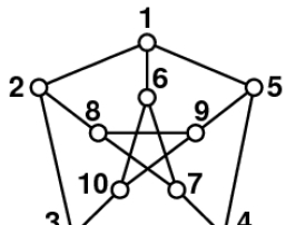
Figure 1: Petersen graph

If we wish to check whether there are stable sets of size four, we take the ideal $I$ generated by the polynomials in Eq. 20, 21 and 22:

$$I = \big{\langle}x_{1}^{2}-x_{1},x_{2}^{2}-x_{2},x_{3}^{2}-x_{3},x_{4}^{2}-x_{4},x_{5}^{2}-x_{5},x_{6}^{2}-x_{6},x_{7}^{2}-x_{7},x_{8}^{2}-x_{8},x_{9}^{2}-x_{9},x_{10}^{2}-x_{10},$$

$$\hskip 5.0ptx_{1}x_{6},x_{2}x_{8},x_{3}x_{10},x_{4}x_{7},x_{5}x_{9},x_{1}x_{2},x_{2}x_{3},x_{3}x_{4},x_{4}x_{5},x_{1}x_{5},x_{6}x_{7},x_{7}x_{8},x_{8}x_{9},x_{9}x_{10},x_{6}x_{10},$$

$$\hskip 5.0ptx_{1}+x_{2}+x_{3}+x_{4}+x_{5}+x_{6}+x_{7}+x_{8}+x_{9}+x_{10}-4\big{\rangle}.$$

By construction, we know that the quotient ring $R:=\mathbb{C}[x_{1},\dots,x_{10}]/I$ is a finite-dimensional $\mathbb{C}$-vector space. Because the ideal $I$ is radical, its dimension equals the number of stable sets of cardinality four in the Petersen graph (not taking symmetries into account). Using Gröbner bases, we find that the monomials $1,x_{10},x_{9},x_{8},x_{7}$ form a vector-space basis of $R$ and that there are no solutions with cardinality five; thus $\alpha(\text{Petersen})=4$ . It is important to stress that we can recover the five different maximum-cardinality stable sets from the knowledge of the complex finite-dimensional vector space basis of $R$ (see [8]).

Next we establish similar encodings for the combinatorial problems stated in Theorem 1.1.

2.1 Proof of Theorem 1.1

Proof 2.4 (Proof (Theorem 1.1, Part 1).).

Suppose that a cycle $C$ of length $L$ exists in the graph $G$ . We set $y_{i}=1$ or $0$ depending on whether node $i$ is on $C$ or not. Next, starting the numbering at any node of $C$ , we set $x_{i}=j$ if node $i$ is the $j$-th node of $C$ . It is easy to check that Eqs. 1 and 2 are satisfied.

To verify Eq. 3, note that since $C$ has length $L$ , if vertex $i$ is the $j$-th node of the cycle, then one of its neighbors, say $k$ , must be the “follower”, namely the $(j+1)$-th element of the cycle. If $j<L$ , then the factor $(x_{i}-x_{k}-1)=0$ appears in the product equation associated with the $i$-th vertex, and the product is zero. If $j=L$ , then the factor $(x_{i}-x_{k}-(L-1))=0$ appears, and the product is again 0. Since this is true for all vertices that are turned “on”, and for all vertices that are “off”, we have Eq. 3 automatically equal to zero, all of the equations of the polynomials vanish.

Conversely, from a solution of the system above, we see that $L$ variables $y_{i}$ are not zero; call this set $C$ . We claim that the nodes $i\in C$ must form a cycle. Since $y_{i}\not=0$ , the polynomial of Eq. 3 must vanish; thus for some $j\in C$ ,

$$(x_{i}-x_{j}+1) =0~{},\quad\text{or}\quad(x_{i}-x_{j}-(L-1))=0~{}.$$

Note that Eq. 3 reduces to this form when $y_{i}=1$ . Therefore, either vertex $i$ is adjacent to a vertex $j$ (with $y_{j}=1$) such that $x_{j}$ equals the next integer value ($x_{i}+1=x_{j}$), or $x_{i}-L=x_{j}-1$ (again, with $y_{j}=1$). In the second case, since $x_{i}$ and $x_{j}$ are integers between 1 and $L$ , this forces $x_{i}=L$ and $x_{j}=1$ . By the pigeonhole principle, this implies that all integer values from 1 to $L$ must be assigned to some node in $C$ starting at vertex 1 and ending at $L$ (which is adjacent to the node receiving $1$).

We have the following corollary.

Corollary 2.5.

A graph $G$ has a hamiltonian cycle if and only if the following zero-dimensional system of $2n$ equations has a solution. For every node $i\in V(G)$ , we have two equations:

$$\prod_{s=1}^{n}(x_{i}-s)=0~{},\quad\text{and}\quad\prod_{j\in Adj(i)}(x_{i}-x_{j}+1)(x_{i}-x_{j}-(n-1))=0~{}.$$

The number of hamiltonian cycles in the graph $G$ equals the number of solutions of the system divided by $2n$ .

Proof 2.6.

Clearly when $L=n$ we can just fix all $y_{i}$ to $1$ , thus many of the equations simplify or become obsolete. We only have to check the last statement on the number of hamiltonian cycles. For that, we remark that no solution appears with multiplicity because the ideal is radical. That the ideal is radical is implied by the fact that every variable appears as the only variable in a unique square-free polynomial (see page 246 of [19]). Finally, note for every cycle there are $n$ ways to choose the initial node to be labeled as $1$ , and then two possible directions to continue the labeling.

Note that similar results can be established for the directed graph version, thus one can consider paths or cycles with orientation. Also note that, we can use the polynomials systems above to investigate the distribution of cycle lengths in a graph (similarly for path lengths and cut sizes). This topic has several outstanding questions. For example, a still unresolved question of Erdös and Gyárfás [35] asks: If $G$ is a graph with minimum-degree three, is it true that $G$ always has a cycle having length that is a power of two? Define the cycle-length polynomial as the square-free univariate polynomial whose roots are the possible cycle lengths of a graph (same can be done for cuts). Considering $L$ as a variable, the reduced lexicographic Gröbner basis (with $L$ the last variable) computation provides us with a unique univariate polynomial on $L$ that is divisible by the cycle-length polynomial of $G$ .

Now we proceed to the proof of part 2 of Theorem 1.1. For this we recall Schnyder’s characterization of planarity in terms of the dimension of a poset [33]: For an $n$-element poset $P$ , a linear extension is an order preserving bijection $\sigma:P\rightarrow\{1,2,\dots,n\}$ . The poset dimension of P is the smallest integer $t$ for which there exists a family of $t$ linear extensions $\sigma_{1},\dots,\sigma_{t}$ of $P$ such that $x<y$ in P if and only if $\sigma_{i}(x)<\sigma_{i}(y)$ for all $\sigma_{i}$ . The incidence poset $P(G)$ of a graph $G$ with node set V and edge set E is the partially ordered set of height two on the union of nodes and edges, where we say $x<y$ if $x$ is a node and $y$ is an edge, and $y$ is incident to $x$ .

Lemma 2.7 (Schnyder’s theorem [33]).

A graph $G$ is planar if and only if the poset dimension of $P(G)$ is no more than three.

Thus our first step is to encode the linear extensions and the poset dimension of a poset $P$ in terms of polynomial equations. The idea is similar to our characterization of cycles via permutations.

Lemma 2.8.

The poset $P=(E,>)$ has poset dimension at most $p$ if and only if the following system of equations has a solution:

For $k=1,\dots,p:$

$$\prod_{s=1}^{|E|}(x_{i}(k)-s)=0,\quad\text{for every $i\in\{1,\ldots,|E|\}$},\quad\quad\text{and}\quad s_{k}\bigg{(}\prod_{\stackrel{{\scriptstyle\{i,j\}\in\{1,\ldots,|E|\},}}{{i<j}}}x_{i}(k)-x_{j}(k)\bigg{)}=1~{}.$$ (23)

For $k=1,\dots,p$ , and every ordered pair of comparable elements $e_{i}>e_{j}$ in $P$ :

$$x_{i}(k)-x_{j}(k)-\Delta_{ij}(k) =0.$$ (24)

For every ordered pair of incomparable elements of $P$ (i.e., $e_{i}\not>e_{j}$ and $e_{j}\not>e_{i}$) :

$$\prod_{k=1}^{p}\big{(}x_{i}(k)-x_{j}(k)-\Delta_{ij}(k)\big{)} =0~{},\quad\quad\prod_{k=1}^{p}\big{(}x_{j}(k)-x_{i}(k)-\Delta_{ji}(k)\big{)}=0~{},$$ (25)

For $k=1,\dots,p$ , and for every pair $\{i,j\}\in\{1,\ldots,|E|\}$:

$$\prod_{d=1}^{|E|-1}(\Delta_{ij}(k)-d)=0,\quad\quad\prod_{d=1}^{|E|-1}(\Delta_{ji}(k)-d)=0~{}.$$ (26)

Proof 2.9.

With Eqs. 23 and 24, we assign distinct numbers 1 through $|E|$ to the poset elements, such that the properties of a linear extension are satisfied. Eqs. 23 and 24 are repeated $p$ times, so $p$ linear extensions are created. If the intersection of these extensions is indeed equal to the original poset $P$ , then for every incomparable pair of elements in $P$ , at least one of the $p$ linear extensions must detect the incomparability. But this is indeed the case for Eq. 25, which says that for the $l$-th linear extension, the values assigned to the incomparable pair $e_{i},e_{j}$ do not satisfy $x_{i}(l)<x_{j}(l)$ , but instead satisfy $x_{j}(l)>x_{i}(l)$ .

Proof 2.10 (Proof (Theorem 1.1, Part 2).).

We simply apply the above lemma to the particular pairs of order relations of the incidence poset of the graph. Note that in the formulation we added variables $z_{\{ij\}}$ that have the effect of turning on or off an edge of the input graph.

Example 2.11 (Posets and Planar Graphs)

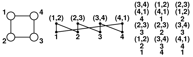
Figure 2: Via Schnyder’s theorem, the square is planar since $P(\text{square})$ has dimension at most three.

Proof 2.12 (Proof (Theorem 1.1, Part 3).).

Using Lemma 2.1, we can finish the proof of Part 3. For a $k$-colorable subgraph $H$ of size $R$ , we set $y_{ij}=1$ if edge $\{i,j\}\in E(H)$ or $y_{ij}=0$ otherwise. By Lemma 2.1, the resulting subsystem of equations has a solution. Conversely from a solution, the subgraph $H$ in question is read off from those $y_{ij}\not=0$ . Solvability implies that $H$ is $k$-colorable.

Before we prove Theorem 1.1, Part 4, we recall that the edge-chromatic number of a graph is the minimum number of colors necessary to color every edge of a graph such that no two edges of the same color are incident on the same vertex.

Proof 2.13 (Proof (Theorem 1.1, Part 4).).

If the system of equations has a solution, then Eq. 18 insures that all variables $x_{ij}$ are assigned $\Delta$ roots of unity. Eq. 19 insures that no node is incident on two edges of the same color. Since the graph contains a vertex of degree $\Delta$ , the graph cannot have an edge-chromatic number less than $\Delta$ , and since the graph is edge-$\Delta$-colorable, this implies that the graph has edge-chromatic number exactly $\Delta$ . Conversely, if the graph has an edge-$\Delta$-coloring, simply map the coloring to the $\Delta$ roots of unity and all equations are satisfied. Since Vizing’s classic result shows that any graph with maximum vertex degree $\Delta$ can be edge-colored with at most $\Delta+1$ colors, if there is no solution, then the graph must have an edge-chromatic number of $\Delta+1$ .

2.2 Normal forms and Dual colorings

In [2] Alon and Tarsi show another polynomial encoding of $k$-colorability. Here we consider one curious consequence of the polynomial method for graph colorings when we use an algebraic encoding similar to that of [2]. By taking a closer look at the normal form of the polynomials involved, we can derive a notion of dual coloring, which has the nice property that a graph is dually $d$-colorable if and only if it is $d$-colorable. This gives rise to an appealing new graph invariant: the simultaneous chromatic number $\sigma(G)$ , defined to be the infimal $d$ such that $G$ has a $d$-labeling that is simultaneously a coloring and a dual coloring.

Fix a graph $G=(V,E)$ with $V:=\{1,\dots,n\}$ and $E\subseteq{V\choose 2}$ , fix a positive integer $d$ , and let $D:=\{0,1\dots,d-1\}$ . Let $\alpha:=\exp({{2\pi i}\over d})\in\mathbb{C}$ be the primitive complex $d$-th root of unity, so that $\alpha^{0},\dots,\alpha^{d-1}$ are distinct and $\alpha^{d}=1$ . For a $d$-labeling $c:V\longrightarrow D$ of the vertices of $G$ , let

$$\epsilon(c):=\prod\left\{(\alpha^{c(i)}-\alpha^{c(j)})\,:\,i<j,\ \{i,j\}\in E\right\}~{}.$$

Clearly, $c$ is a proper $d$-coloring of $G$ if and only if $\epsilon(c)\neq 0$ .

With every orientation $O=(V,A)$ of $G$ (where $A$ denotes the set of “arrows” or directed edges) associate a sign $\mbox{sign}^{O}=\pm 1$ defined by the parity of the number $|\{(i,j)\in A\,:\,i>j\}|$ of flips of $O$ from the standard orientation (where every directed edge $(i,j)$ has $i<j$), and an out-degree vector $\delta^{O}:=(\delta^{O}_{1},\dots,\delta^{O}_{n})$ with $\delta^{O}_{i}$ the out-degree of vertex $i$ in $O$ . For a non-negative integer $k$ let $[k]\in D$ be the representative of $k$ modulo $d$ , and for a vector $\delta=(\delta_{1},\dots,\delta_{n})\in V^{n}$ let $[\delta]=([\delta_{1}],\dots,[\delta_{n}])\in D^{V}$ . For a labeling $c^{*}:V\longrightarrow D$ of the vertices of $G$ let

$$\epsilon^{*}(c^{*}):=\sum\,\left\{\,\mbox{sign}^{O}\ :\ \mbox{$O$ orientation of $G$ with $[\delta^{O}]=c^{*}$}\,\right\}~{}.$$

Call $c^{*}$ a dual $d$-coloring of $G$ if $\epsilon^{*}(c^{*})\neq 0$ .

Theorem 2.14.

A graph has a $d$-coloring, namely $c\in D^{V}$ with $\epsilon(c)\neq 0$ (so is $d$-colorable) if and only if it has a dual $d$-coloring, namely $c^{*}\in D^{V}$ with $\epsilon^{*}(c^{*})\neq 0$ (so is dually $d$-colorable).

Proof 2.15.

Let $G$ be a graph on $n$ vertices. Consider the following radical zero-dimensional ideal $I$ in $\mathbb{C}[x_{1},\dots,x_{n}]$ and its variety $\text{variety}(I)$ in $\mathbb{C}^{n}$:

$$I\ :=\ \langle x_{1}^{d}-1,\dots,x_{n}^{d}-1\rangle\ ,\quad\text{variety}(I)\ :=\ \{\,\alpha^{c}:=(\alpha^{c(1)},\dots,\alpha^{c(n)})\in\mathbb{C}^{n}\ :\ c\in D^{V}\,\}\ .$$

It is easy to see that the set $\{x_{1}^{d}-1,\dots,x_{n}^{d}-1\}$ is a universal Gröbner basis (see [3] and references therein). Thus, the (congruence classes of) monomials $x^{c^{*}},\ c^{*}\in D^{V}$ (where $x^{c^{*}}:=\prod_{i=1}^{n}x_{i}^{c^{*}(i)}$), which are those monomials not divisible by any $x_{i}^{d}$ , form a vector space basis for the quotient $\mathbb{C}[x_{1},\dots,x_{n}]/I$ . Therefore, every polynomial $f=\sum a_{\delta}\cdot x^{\delta}$ has a unique normal form $[f]$ with respect to this basis, namely the polynomial that lies in the vector space spanned by the monomials $x^{c^{*}},\ c^{*}\in D^{V}$ , and satisfies $f-[f]\in I$ . It is not very hard to show that this normal form is given by $[f]=\sum a_{\delta}\cdot x^{[\delta]}$ .

Now consider the graph polynomial of $G$ ,

$$f_{G}:=\prod\left\{\,(x_{i}-x_{j})\,:\,i<j,\ \{i,j\}\in E\,\right\}~{}.$$

The labeling $c\in D^{V}$ is a $d$-coloring of $G$ if and only if $\epsilon(c)=f_{G}(\alpha^{c})\neq 0$ . Thus, $G$ is not $d$-colorable if and only if $f_{G}$ vanishes on every $\alpha^{c}\in\text{variety}(I),$ which holds if and only if $f\in I,$ since $I$ is radical. It follows that $G$ is $d$-colorable if and only if the representative of $f_{G}$ is not zero. Since $f_{G}=\sum\mbox{sign}^{O}\cdot x^{\delta^{O}}$ , with the sum extending over the $2^{|E|}$ orientations $O$ of $G$ , we obtain

$$[f_{G}]=\sum\mbox{sign}^{O}\cdot x^{[\delta^{O}]}=\sum_{c^{*}\in D^{V}}\epsilon^{*}(c^{*})\cdot x^{c^{*}}~{}.$$

Therefore $[f_{G}]\neq 0$ and $G$ is $d$-colorable if and only if there is a $c^{*}\in D^{V}$ with $\epsilon^{*}(c^{*})\neq 0$ .

Example 2.16

Consider the graph $G=(V,E)$ having $V=\{1,2,3,4\}$ and $E=\{12,13,23,24,34\}$ , and let $d=3$ . The normal form of the graph polynomial can be shown to be

$$[f_{G}] = x_{1}^{2}x_{2}^{2}x_{3}-x_{1}^{2}x_{2}^{2}x_{4}+x_{1}^{2}x_{2}x_{4}^{2}-x_{1}^{2}x_{2}x_{3}^{2}+x_{1}^{2}x_{3}^{2}x_{4}-x_{1}^{2}x_{3}x_{4}^{2}+x_{1}x_{2}-x_{1}x_{2}x_{3}^{2}x_{4}+x_{1}x_{3}^{2}x_{4}^{2}$$

$$-x_{1}x_{3}+x_{1}x_{2}^{2}x_{3}x_{4}-x_{1}x_{2}^{2}x_{4}^{2}+x_{3}^{2}-x_{3}x_{4}+x_{2}^{2}x_{3}x_{4}^{2}-x_{2}^{2}+x_{2}x_{4}-x_{2}x_{3}^{2}x_{4}^{2}\ .$$

Note that in general, the number of monomials appearing in the expansion of $f_{G}$ can be as much as the number of orientations $2^{|E|}$; but usually it will be smaller due to cancellations that occur. Moreover, there will usually be further cancellations when moving to the normal form, so typically $[f_{G}]$ will have fewer monomials. In our example, out of the $2^{|E|}=2^{5}=32$ monomials corresponding to the orientations, in the expansion of $f_{G}$ only $20$ appear, and in the normal form $[f_{G}]$ only $18$ appear due to the additional cancellation:

$$-[x_{1}x_{3}^{3}x_{4}]+[x_{1}x_{2}^{3}x_{4}]=-x_{1}x_{4}+x_{1}x_{4}=0~{}.$$

Note that the graph $G$ in this example has only six $3$-colorings (which are in fact the same up to relabeling of the colors), but as many as $18$ dual $3$-colorings $c^{*}$ corresponding to monomials $x^{c^{*}}$ appearing in $[f_{G}]$ . For instance, consider the labeling $c^{*}(1)=c^{*}(2)=c^{*}(4)=0,\ c^{*}(3)=2$: the only orientation $O$ that satisfies $[\delta^{O}_{j}]=c^{*}(j)$ for all $j$ is one with edges oriented as $21,23,24,31,34$ , having $\mbox{sign}^{O}=1$ and out-degrees $\delta^{O}_{1}=\delta^{O}_{4}=0$ , $\delta^{O}_{3}=2$ and $\delta^{O}_{2}=3$ , contributing to $[f_{G}]$ the non-zero term $\epsilon^{*}(c^{*})\cdot\prod_{j=1}^{4}x_{j}^{c^{*}(j)}=1\cdot x_{1}^{0}x_{2}^{0}x_{3}^{2}x_{4}^{0}=x_{3}^{2}$ . Thus, $c^{*}$ is a dual $3$-coloring (but, since $c^{*}(1)=c^{*}(2)$ , it is neither a usual $3$-coloring nor a simultaneous $3$-coloring — see below).

Note that in this example, and seemingly often, there are many more dual colorings than colorings; this suggests a randomized heuristic to find a dual $d$-coloring for verifying $d$-colorability.

A particularly appealing notion that arises is the following: call a vertex labeling $s:V\longrightarrow D$ a simultaneous $d$-coloring of a graph $G$ if it is simultaneously a $d$-coloring and a dual $d$-coloring of $G$ . The simultaneous chromatic number $\sigma(G)$ is then the minimum $d$ such that $G$ has a simultaneous $d$-coloring. This is a strong notion that may prove useful for inductive arguments, perhaps in the study of the 4-color problem of planar graphs, and which provides an upper bound on the usual chromatic number $\chi(G)$ . First note that, like the usual chromatic number, it can be bounded in terms of the maximum degree $\Delta(G)$ as follows.

Theorem 2.17.

The simultaneous chromatic number of any graph $G$ satisfies  $\sigma(G)\leq\Delta(G)+1$ . Moreover, for any $G$ and $d\geq\Delta(G)+1$ , there is an acyclic orientation $O$ whose out-degree vector $\delta^{O}=(\delta^{O}_{1},\dots,\delta^{O}_{n})$ provides a simultaneous $d$-coloring $s$ defined by $s(i):=\delta^{O}_{i}$ for every vertex $i$ .

Proof 2.18.

We prove the second (stronger) claim, by induction on the number $n$ of vertices. For $n=1$, this is trivially true. Suppose $n>1$ , and let $d:=\Delta(G)+1$ . Pick any vertex $i$ of maximum degree $\Delta(G)$ , and let $G^{\prime}$ be the graph obtained from $G$ by removing vertex $i$ and all edges incident on $i$ . Let $O^{\prime}$ be an acyclic orientation of $G^{\prime}$ and $s^{\prime}$ the corresponding simultaneous $d$-coloring of $G^{\prime}$ guaranteed to exist by induction. Extend $O^{\prime}$ to an orientation $O$ of $G$ by orienting all edges incident on $i$ away from $i$ , and extend $s$ to the corresponding vertex labeling of $G$ by setting $s(i):=\delta^{O}_{i}=d-1$ . Then $O$ is acyclic, and therefore $O$ is the unique orientation of $G$ with out-degree vector $\delta^{O}$ . Thus,

$$\epsilon^{*}(s)\ =\ \sum\,\{\,\mbox{sign}^{\theta}\,:\,\mbox{$\theta$ orientation of $G$ with $[\delta^{\theta}]=s=\delta^{O}$}\,\}\ =\ \pm 1\ \neq\ 0\ ,$$

and therefore $s$ is a dual $d$-coloring of $G$ . Moreover, if $j$ is any neighbor of $i$ in $G$ , then the degree of $j$ in $G^{\prime}$ is at most $d-2$ , and therefore its label $s^{\prime}(j)=\delta^{O^{\prime}}(j)\leq d-2$ , and hence $s(j)=s^{\prime}(j)\neq d-1=s(i)$ . Therefore, $s$ is also a $d$-coloring of $G$ , completing the induction.

Example 2.19 (simultaneous 4-coloring of the Petersen graph)

According to Figure 3, $\delta^{O}=(2,1,0,2,0,3,1,2,3,1)$ . By inspection of Figure 3, $s(i):=\delta_{i}^{O}$ does indeed describe a valid 4-coloring of the Petersen graph.

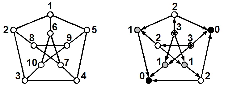
Figure 3: Left: A vertex labeling. Right: An acyclic orientation labeled with out-degrees.

There are many fascinating new combinatorial and computational problems related to this new graph invariant, the behavior of which is quite different from that of the usual chromatic number. For instance, the direct analog of Brooks’ theorem, which states that every connected graph with maximum degree $\Delta$ that is neither complete nor an odd cycle is $\Delta$-colorable, fails: It is not hard to verify that the simultaneous chromatic number of the cycle $C_{n}$ is $2$ if and only if $n$ is a multiple of $4$; thus, the hexagon satisfies $\sigma(C_{6})=3>\Delta(C_{6})$ . Which are the simultaneous chromatic Brooks graphs, i.e. those with $\sigma(G)=\Delta(G)$ ? What is the complexity of deciding if a graph is simultaneously $d$-colorable? Which graphs are simultaneously $d$-colorable for small $d$ ? For $d=2$ , the complete answer was given by L. Lovász [25] during a discussion at the Oberwolfach Mathematical Institute:

Theorem 2.20.

(Lovász) A connected bipartite graph $G=(A,B,E)$ has simultaneous chromatic number $\sigma(G)=2$ if and only if at least one of $|A|$ and $|B|$ has the same parity as $|E|$ .

3 Nullstellensatz Degree Growth in Combinatorics

The Hilbert Nullstellensatz states that a system of polynomial equations $\left\{f_{1}(x)=0,f_{2}(x)=0,\dots,f_{r}(x)=0\right\}\subseteq\mathbb{C}[x_{1},\ldots,x_{n}]$ has no solution in ${\mathbb{C}}^{n}$ if and only if there exist polynomials $\alpha_{1},\dots,\alpha_{r}\in{\mathbb{C}}[x_{1},\dots,x_{n}]$ such that $1=\sum\alpha_{i}f_{i}$ (see [7]). The purpose of this section is to investigate the degree growth of the coefficients $\alpha_{i}$ . In particular, systems of polynomials coming from combinatorial optimization.

In our investigations, we will often need to find explicit Nullstellensatz certificates for specific graphs. This can be done via linear algebra. First, given a system of polynomial equations, fix a tentative degree for the coefficient polynomials $\alpha_{i}$ in the Nullstellensatz certificates. This yields a linear system of equations whose variables are the coefficients of the monomials of the polynomials $\alpha_{1},\dots,\alpha_{r}$ . Then, solve this linear system. If the system has a solution, we have found a Nullstellensatz certificate. Otherwise, try a higher degree for the polynomials $\alpha_{i}$ . For the Nullstellensatz certificates, the degrees of the polynomials $\alpha_{i}$ cannot be more than known bounds (see e.g., [18] and references therein), thus this is a finite (but potentially long) procedure to decide whether a system of polynomials is feasible or not. In practice, sometimes low degrees suffice to find a certificate.

Example 3.1

Suppose we wish to test $K_{4}$ for 3-colorability, and we assume that the $\alpha_{i}$ in the Nullstellensatz certificate have degree 1. After encoding $K_{4}$ with the system of polynomial equations, we “conjecture” that there exists a Nullstellensatz certificate of the following form

$$1 =(c_{1}x_{1}+c_{2}x_{2}+c_{3}x_{3}+c_{4}x_{4}+c_{5})(x_{1}^{3}-1)+(c_{6}x_{1}+c_{7}x_{2}+c_{8}x_{3}+c_{9}x_{4}+c_{10})(x_{2}^{3}-1)$$

$$\quad+(c_{11}x_{1}+\cdots+c_{15})(x_{3}^{3}-1)+(c_{16}x_{1}+\cdots+c_{20})(x_{4}^{3}-1)$$

$$\quad+(c_{21}x_{1}+\cdots+c_{25})(x_{1}^{2}+x_{1}x_{2}+x_{2}^{2})+(c_{26}x_{1}+\cdots+c_{30})(x_{1}^{2}+x_{1}x_{3}+x_{3}^{2})$$

$$\quad+(c_{31}x_{1}+\cdots+c_{35})(x_{1}^{2}+x_{1}x_{4}+x_{4}^{2})+(c_{36}x_{4}+\cdots+c_{40})(x_{2}^{2}+x_{2}x_{3}+x_{3}^{2})$$

$$\quad+(c_{41}x_{1}+\cdots+c_{45})(x_{2}^{2}+x_{2}x_{4}+x_{4}^{2})+(c_{46}x_{1}+\cdots+c_{50})(x_{3}^{2}+x_{3}x_{4}+x_{4}^{2}).$$

When we multiply out this certificate, we group together like powers of $x_{1},x_{2},x_{3},x_{4}$ as follows:

$$1 =c_{1}x_{1}^{4}+\cdots+c_{13}x_{3}^{4}+\cdots+c_{8}x_{2}^{3}x_{3}+\cdots+(c_{22}+c_{21}+c_{27}+c_{32})x_{1}^{2}x_{2}+\cdots$$

$$\quad+(c_{35}+c_{45}+c_{50})x_{4}^{2}+\cdots+(-c_{15}-c_{20}-c_{5}-c_{10}).$$

Because the Nullstellensatz certificate is identically 1, this identity gives rise to the following system of linear equations: $0=c_{1},0=c_{13},0=c_{8},0=c_{22}+c_{21}+c_{27}+c_{32},0=c_{35}+c_{45}+c_{50},\dots,1=-c_{15}-c_{20}-c_{5}-c_{10}$ . In other words, we have a large-scale sparse system of linear equations that consists only of 1s and $-1$s. We implemented an exact-arithmetic linear system solver. In this example, it turns out that degree 1 is not sufficient for generating a Nullstellensatz certificate — that is, this linear system has no solution. Ultimately, we discovered that degree four is required, and we were able to produce the following certificate:

$$1 =(-x_{1}^{3}-1)(x_{1}^{3}-1)+\bigg{(}\frac{4}{9}x_{4}^{4}-\frac{5}{9}x_{4}^{3}x_{2}-\frac{2}{9}x_{4}^{3}x_{3}-\frac{4}{9}x_{4}^{3}x_{1}+\frac{2}{9}x_{4}^{2}x_{2}x_{1}+\frac{2}{9}x_{4}^{2}x_{3}x_{1}\bigg{)}(x_{4}^{2}+x_{2}x_{4}+x_{2}^{2})$$

$$\phantom{=}+\bigg{(}\frac{1}{9}x_{4}^{4}+\frac{2}{9}x_{4}^{3}x_{2}-\frac{1}{9}x_{4}^{3}x_{1}-\frac{2}{9}x_{4}^{2}x_{2}x_{1}\bigg{)}(x_{2}^{2}+x_{3}x_{2}+x_{3}^{2})+\bigg{(}\frac{2}{9}x_{4}^{4}+\frac{1}{9}x_{4}^{3}x_{2}+\frac{1}{9}x_{4}^{3}x_{1}+\frac{2}{9}x_{4}^{2}x_{2}x_{1}\bigg{)}(x_{4}^{2}+x_{3}x_{4}+x_{3}^{2})$$

$$\phantom{=}+\bigg{(}-\frac{2}{3}x_{4}^{4}+x_{4}^{3}x_{1}-x_{4}x_{1}^{3}+x_{1}^{4}\bigg{)}(x_{4}^{2}+x_{1}x_{4}+x_{1}^{2})+\frac{1}{3}x_{4}^{3}x_{2}(x_{2}^{2}+x_{1}x_{2}+x_{1}^{2})+\bigg{(}-\frac{1}{3}x_{4}^{4}-\frac{1}{3}x_{4}^{3}x_{2}\bigg{)}(x_{3}^{2}+x_{1}x_{3}+x_{1}^{2}).$$

Lemma 3.2.

If $\text{P}\neq\text{NP}$ , then there must exist an infinite family of graphs whose minimum-degree non-3-colorability Nullstellensatz certificates have unbounded growth with respect to the number of vertices and edges in the graph.

Proof 3.3.

Our proof is by contradiction with the hypothesis $\text{P}\neq\text{NP}$ . Consider a non-3-colorable graph that has been encoded as the system of polynomial equations $(x_{i}^{3}-1)=0$ for $i\in V(G)$ , and $(x_{i}^{2}+x_{i}x_{j}+x_{j}^{2})=0$ for $\{i,j\}\in E(G)$ . Assume that every minimum-degree non-3-colorability Nullstellensatz certificate has $\deg(\alpha_{i})<d$ for some constant $d$ . We will show that $\text{P}=\text{NP}$ by providing a polynomial-time algorithm for solving Graph-3-Coloring: (1) Given a graph $G$ , encode it as the above system of polynomial equations, (2) Construct and solve the associated linear system for monomials of degree $<d$ , (3) If the system has a solution, a Nullstellensatz certificate exists, and the graph is non-3-colorable: Return no, (4) If the system does not have a solution, there does not exist a Nullstellensatz certificate, and the graph is 3-colorable: Return yes.

Now we analyze the running time of this algorithm. In Step 1, our encoding has one polynomial equation per vertex and one polynomial equation per edge. Since there are $O(n^{2})$ edges in a graph, our polynomial system has $n+n^{2}=O(n^{2})$ equations. Since every equation only contains coefficients $\pm 1$ and is of degree three or less, encoding the graph as the above system of polynomial equations clearly runs in polynomial-time.

For Step 2, we note that by Corollary 3.2b of [34], if a system of linear equations $Ax=b$ has a solution, then it has a solution polynomially-bounded by the bit-sizes of the matrix $A$ and the vector $b$ (see [34] for a definition of bit-size). In this case, the vector $b$ contains only zeros and ones. To calculate the bit-size of $A$ , we recall our assumption that, for every $\alpha_{i}$ , $\deg(\alpha_{i})<d$ for some constant $d$ . Therefore, an upper bound on the number of terms in each $\alpha_{i}$ is the total number of monomials in $n$ variables of degree less than or equal to $d$ . Therefore, the number of terms in each $\alpha_{i}$ is

$$\binom{n+d-1}{n-1}+\binom{n+d-2}{n-1}+\cdots+\binom{n-1}{n-1} =O(n^{d})+O(n^{d-1})+\cdots+O(1)=O(n^{d}).$$

Since there are $O(n^{2})$ equations, there are at most $O(n^{d+2})$ unknowns in the linear system, and thus, $O(n^{d+2})$ columns in $A$ . Since the vertex equations $(x_{i}^{3}-1)=0$ have two terms, and the edge equations $(x_{i}^{2}+x_{i}x_{j}+x_{j}^{2})=0$ have 3 terms, there are $O(n^{d+2})$ terms in the expanded Nullstellensatz certificate, and $O(n^{d+2})$ rows in $A$ . Since entries in $A$ are $0,\pm 1$ , the matrix $A$ contains only entries of bit-size at most 2. Therefore, the bit-sizes of both $A$ and $b$ are polynomially-bounded in $n$ , and by Theorem 3.3 of [34], the linear system can be solved in polynomial-time.

Therefore, we have demonstrated a polynomial-time algorithm for solving Graph-3-Coloring, and since Graph-3-Coloring is NP-Complete ([12]), this implies $\text{P}=\text{NP}$ , which contradicts our hypothesis. Therefore, $\deg(\alpha_{i})\nleq d$ for any constant $d$ .

Thus, in the linear algebra approach to finding a minimum-degree Nullstellensatz certificate, the existence of a universal constant bounding the degree is impossible under a well-known hypothesis of complexity theory. Clearly, a similar result can be obtained for other encodings (for a generalized statement see [26]). Note that the linear algebra method does not rely on any property that is unique to a particular combinatorial or NP-Complete problem; the only assumption is that the problem can be represented as a system of polynomial equations. We will use it to find Nullstellensatz certificates of non-3-colorability and sizes of stable sets of graphs.

We remark that this linear algebra method finds not only a Nullstellensatz certificate (if it exists), but it finds one of minimum possible degree. With our implementation, we ran several experiments. We quickly found out that the systems of linear equations are numerically unstable, thus it is best to use exact arithmetic to solve them. The systems of linear equations are also quite large in practice, as the bound on the degree of the polynomial coefficients grows. Thus we need ways to reduce the number of unknowns.

We will not discuss here ad hoc methods that depend on the particular polynomial system at hand (see [26] for methods specific to $3$-colorability), but one rather useful general trick is to randomly eliminate variables in the above procedure. Instead of allowing all monomials of degree $\leq d$ to appear in the construction of the linear system of equations, we can randomly set unknowns in the linear system of equations to $0$ — e.g., set each variable to 0 with probability $p$ , independently, to get a smaller system.

Figure 4: Probability tests on cliques and odd wheels.

In Figure 4, we see the results of the probabilistic search for smaller Nullstellensatz certificates. On the $x$-axis is the probability $p$ of keeping an unknown in the linear system. Thus, if $p=0.1$ , 90% of the time we set the unknown to 0, and only 10% of the time, we keep it in the system. For the cliques and odd wheels, we know that there is always a certificate of degree four. For every probability $0.1,0.2,\ldots,1$ we performed 100 searches for a degree four certificate. For both the cliques and the odd wheels, at $p=0.1$ and $p=0.2$ , we almost never found a certificate. But for $p=0.4$ , we found certificates 95% of the time. In practice this idea is useful. We can reduce the number of variables in the linear system by 60%, and still find a Nullstellensatz certificate 90% of the time. We will report the results of specific computations in Section 3.2.

3.1 The Nullstellensatz and Stable Sets of Graphs

Lovász [24] stated the challenge of finding an explicit family of graphs with growth in the degree of Nullstellensatz certificates. Here we solve his challenge. Our main result is stated in Theorem 1.2: For every graph $G$ , there exists a Nullstellensatz certificate of degree $\alpha(G)$ , the stability number of $G$ , certifying that $G$ has no stable set of size $>\alpha(G)$ . Moreover, this is the minimum possible degree for all graphs. In what follows, for any graph $G$ with stability number $\alpha(G)$ and integer $r\geq 1$ , we associate the infeasible system of polynomial equations $J(G,r)$ :

$$-(\alpha(G)+r)+\sum_{i=1}^{n}x_{i}=0~{},$$ (27)

$$x_{i}^{2}-x_{i}=0,\mbox{ for every node }i\in V(G)~{},$$ (28)

$$x_{i}x_{j}=0,\hbox{ for every edge }\{i,j\}\in E(G)~{}.$$ (29)

Thus, the Nullstellensatz certificate will have the general form:

$$1=A\bigg{(}-(\alpha(G)+r)+\sum_{i=1}^{n}x_{i}\bigg{)}+\sum_{i\in V(G)}Q_{i}(x_{i}^{2}-x_{i})+\sum_{\{i,j\}\in E(G)}Q_{ij}(x_{i}x_{j})~{}.$$ (30)

In the rest of this section, we will refer to the coefficient polynomials using these particular letters (i.e. $A,Q_{i}$ , etc).

Definition 3.4

A Nullstellensatz certificate (Eq. 30) has degree $d$ if $\max\{deg(A),deg(Q_{i}),deg(Q_{ij})\}=d$ .

Lemma 3.5.

For any graph $G$ and a Nullstellensatz certificate

$$1 =A\underbrace{\bigg{(}-(\alpha(G)+r)+\sum_{i=1}^{n}x_{i}\bigg{)}}_{B}+\sum_{i\in V(G)}Q_{i}(x_{i}^{2}-x_{i})+\sum_{\{i,j\}\in E(G)}Q_{ij}(x_{i}x_{j})$$ (31)

certifying that $G$ has no stable set of size $(\alpha(G)+r)$ (with $r\geq 1$), we can construct a “reduced” Nullstellensatz certificate

$$1 =A^{\prime}\bigg{(}-(\alpha(G)+r)+\sum_{i=1}^{n}x_{i}\bigg{)}+\sum_{i\in V(G)}Q^{\prime}_{i}(x_{i}^{2}-x_{i})+\sum_{\{i,j\}\in E(G)}Q^{\prime}_{ij}(x_{i}x_{j}),$$

such that

1. The coefficient $A^{\prime}$ multiplying $-(\alpha(G)+r)+\sum_{i=1}^{n}x_{i}$ has only square-free monomials supported on stable sets of $G$ , and thus $\deg(A^{\prime})\leq\alpha(G)$ .

2. $\max\{deg(A),deg(Q_{i}),deg(Q_{ij})\}=\max\{deg(A^{\prime}),deg(Q^{\prime}_{i}),deg(Q^{\prime}_{ij})\}$ . Thus, if the original Nullstellensatz certificate has minimum-degree, the “reduced” certificate also has minimum-degree.

Proof 3.6.

Let $I$ be the ideal generated by $x_{i}^{2}-x_{i}$ (for every node $i\in V(G)$), and $x_{i}x_{j}$ ( for every edge $\{i,j\}\in E(G)$). We apply reductions modulo $I$ to Eq. 31. If a non-square-free monomial appears in polynomial $A$ , say $x_{i_{1}}^{\alpha_{1}}x_{i_{2}}^{\alpha_{2}}\cdots x_{i_{k}}^{\alpha_{k}}$ with at least one $\alpha_{j}>1$ , then we can subtract the polynomial $x_{i_{1}}^{\alpha_{1}}x_{i_{2}}^{\alpha_{2}}\cdots,x_{i_{j}}^{\alpha_{j}-2}x_{i_{k}}^{\alpha_{k}}B(x_{i_{j}}^{2}-x_{i_{j}})$ from $AB$ and simultaneously add it to $\sum Q_{s}(x_{s}^{2}-x_{s})$ . Thus, eventually we obtain a new certificate that has only square-free monomials in $A^{\prime}$ . Furthermore, if $Q^{\prime}_{s}$ has new monomials, they are of degree less than or equal to what was originally in $A$ .

Similarly, if $x_{i_{1}}x_{i_{2}}\cdots x_{i_{k}}$ appears in $A$ , but $x_{i_{1}}x_{i_{2}}\cdots x_{i_{k}}$ contains an edge $\{i,j\}\in E(G)$ (if $x_{i}x_{j}$ divides $x_{i_{1}}x_{i_{2}}\cdots x_{i_{k}}$), then we can again subtract $B(x_{i_{1}}x_{i_{2}}\cdots x_{i_{k}}/x_{i}x_{j})(x_{i}x_{j})$ from $AB$ , and, at the same time, add it to $\sum_{\{i,j\}\in E(G)}Q_{ij}x_{i}x_{j}$ . Furthermore, the degree is maintained, and we have reached the form we claim exists for $A^{\prime}$ .

We now show that, for every graph, there exists an explicit Nullstellensatz certificate of degree $\alpha(G)$ .

Theorem 3.7.

Given a graph $G$ , there exists a Nullstellensatz certificate of degree $\alpha(G)$ certifying the non-existence of stable sets of size greater than $\alpha(G)$ .

Proof 3.8.

The proof is an algorithm to construct the explicit Nullstellensatz certificate for the non-existence of a stable set of size $\alpha(G)+r$, with $r\geq 1$ . First, let us establish some notation: Let $S(i,G)$ be the set of all stable sets of size $i$ in $G$ . We index nodes in the graph by integers, thus stable sets in $G$ are subsets of integers. When we refer to a monomial $x_{d_{1}}x_{d_{2}}\cdots x_{d_{i}}$ as a “stable set”, we mean $\{d_{1},\ldots,d_{i}\}\in S(i,G)$ . We use “hat” notation to remove a variable from a monomial, meaning $x_{d_{1}}x_{d_{2}}\cdots x_{d_{i-1}}\widehat{x_{d_{i}}}x_{d_{i+1}}\cdots x_{d_{k}}=x_{d_{1}}x_{d_{2}}\cdots x_{d_{i-1}}x_{d_{i+1}}\cdots x_{d_{k}}$ . Finally, let

$$\mathscr{P}(i,G) :=\sum_{\{d_{1},d_{2},\ldots,d_{i}\}\in S(i,G)}x_{d_{1}}x_{d_{2}}\cdots x_{d_{i}}~{},\quad\quad\quad\text{and}\quad\mathscr{P}(0,G):=1~{}.$$

When $\mathscr{P}(i,G)$ is ordered lexicographically, we denote $\mathscr{P}_{j}(i,G)$ as the $j$-th term. We also define the constants

$$C_{i}^{G} :=\frac{iC_{i-1}^{G}}{\alpha(G)+r-i}~{},\quad\quad\text{and}\quad C_{0}^{G}:=\frac{1}{\alpha(G)+r}~{}.$$

Our main claim is that we can construct explicit coefficients $A,Q_{i},Q_{ij}$ of degree less than or equal to $\alpha(G)$ such that the following identity is satisfied

$$1 =A\underbrace{\bigg{(}-(\alpha(G)+r)+\sum_{i=1}^{n}x_{i}\bigg{)}}_{B}+\underbrace{\sum_{\{i,j\}\in E(G)}Q_{ij}x_{i}x_{j}+\sum_{i=1}^{n}Q_{i}(x_{i}^{2}-x_{i})}_{C}~{}.$$

We do so by the algorithm of Figure 5. In Figure 5 and in what follows, $AB$ and $C$ refer to parts of the equation as marked above.

***

***

***

***

***

***

***

***

***

***

***

***

********

ALGORITHM (Nullstellensatz certificate construction)

$\text{INPUT: A graph}\ G(V,E),\ \text{associated polynomials $\mathscr{P}(i,G)$~{},}\ \alpha(G),r$

$\text{OUTPUT: polynomials }(A,Q_{i},Q_{ij})\ \text{such that}\ AB+C=1\text{ is true}$

0

$A\leftarrow-\sum_{i=0}^{\alpha(G)}C_{i}^{G}\mathscr{P}(i,G)$

1

$Q_{i}\leftarrow 0$ , for $i=1\ldots|V|$

2

$Q_{ij}\leftarrow 0$ , for $\{i,j\}\in E(G)$

3

for $i\leftarrow 0\textbf{ to }\alpha(G)$

4

for $j\leftarrow 1\textbf{ to }\text{\# of monomials in $\mathscr{P}(i,G)$}$

5

for $k\leftarrow 1\textbf{ to }|V|$

6

Let $\mathscr{P}_{j}(i,G)=x_{d_{1}}x_{d_{2}}\cdots x_{d_{i}}$

7

if $\mathscr{P}_{j}(i,G)x_{k}$ is a square-free stable set

8

(rule 1) $Q_{k}\leftarrow Q_{k}+C_{i+1}^{G}x_{d_{1}}x_{d_{2}}\cdots x_{d_{i}}$

9

else if $\mathscr{P}_{j}(i,G)x_{k}$ is a square-free non-stable set

10

Choose an edge $l$, $1\leq l\leq i$, so that $(k,d_{l})$ is an edge of $G$

12

(rule 2) $Q_{kd_{l}}\leftarrow Q_{kd_{l}}+C_{i}^{G}x_{d_{1}}x_{d_{2}}\cdots x_{d_{l-1}}\widehat{x_{d_{l}}}x_{d_{l+1}}\cdots x_{d_{i}}$

13

end if

14

end for

15

end for

16

end for

17

return $A,Q_{i},Q_{ij}$

********************************************

Figure 5: Nullstellensatz certificate construction

It is clear that the algorithm terminates for any finite graph, since the number of iterations of each for loop is finite. To prove correctness of the algorithm, we demonstrate that the following statement is true for each iteration of the for loop beginning in line 3:

$$\hbox{Prior to the $m$-th iteration, $AB+C-1$ only contains terms of degree $m+1$ or greater.}\atop\hbox{Furthermore, all terms of degree $m+1$ are square-free.} *$$ ()

When the for loop is initialized, $A$ is set to the polynomial $-\sum_{i=0}^{\alpha(G)}C_{i}^{G}\mathscr{P}(i,G)$ , and $Q_{i},Q_{ij}$ are set to zero. Therefore, prior to the $0$-th iteration, $C=0$ and $AB+C-1=AB-1$ . Since the constant term in $AB$ is equal to

$$-C_{0}^{G}\mathscr{P}(0,G)\big{(}-(\alpha(G)+r)\big{)} =-\frac{1}{\alpha(G)+r}\bigg{(}-(\alpha(G)+r)\bigg{)}=1~{},$$

this implies that $AB-1$ only contains terms of degree 1 or higher. Furthermore, linear terms are by definition square-free. Thus, $(*)$ is true at initialization.

Now we must show that if $(*)$ is true prior to the $m$-th iteration of the for loop, then it will be true prior to the $(m+1)$-th iteration. Assume then, that prior to the $m$-th iteration, $AB+C-1$ only contains terms of degree $m+1$ or greater, and that all terms of degree $m+1$ are square-free. We must show that prior to the $(m+1)$-th iteration, $AB+C-1$ only contains terms of degree $m+2$ or greater, and furthermore, that all terms of degree $m+2$ are square-free. Prior to the $m$-th iteration, there are only two kinds of terms of degree $m+1$ in $AB+C-1$ : (1) terms corresponding to square-free, stable sets, and (2) terms corresponding to square-free, non-stable sets. We will show that both kinds of terms cancel during the $m$-th iteration.

• Let $x_{d_{1}}x_{d_{2}}\cdots x_{d_{m+1}}$ be any square-free, stable set monomial in $AB+C-1$ of degree $(m+1)$ . Since $\{d_{1},d_{2},\ldots,d_{m+1}\}$ is a stable set, all subsets of size $m$ are likewise stable sets and appear as summands in $\mathscr{P}(m,G)$ . Consider the coefficient of $x_{d_{1}}x_{d_{2}}\cdots x_{d_{m+1}}$ in $C$ . During the $m$-th iteration, we apply rule 1 and create this monomial $\binom{m+1}{m}$ times in $C$ . Since this monomial is created by the multiplication of $x_{d_{1}}x_{d_{2}}\cdots\widehat{x_{d_{k}}}\cdots x_{d_{m+1}}$ with $(x^{2}_{d_{k}}-x_{d_{k}})$ , the coefficient for $x_{d_{1}}x_{d_{2}}\cdots x_{d_{m+1}}$ in $C$ is

  $$-\binom{m+1}{m}C_{m+1}^{G} =-(m+1)C_{m+1}^{G}$$

  Now we will calculate the coefficient of this same monomial in $AB$ . This monomial is created in two ways, (1) multiplying $-C_{m}^{G}x_{d_{1}}x_{d_{2}}\cdots x_{d_{j-1}}\widehat{x_{d_{j}}}x_{d_{j+1}}\cdots x_{d_{m+1}}$ by $x_{d_{j}}$ (repeated $(m+1)$ times, once for each $x_{d_{j}}$), or (2) multiplying $-C_{m+1}^{G}x_{d_{1}}x_{d_{2}}\cdots x_{d_{m+1}}$ by $-(\alpha(G)+r)$ (occurring exactly once). Therefore, the coefficient of $x_{d_{1}}x_{d_{2}}\cdots x_{d_{m+1}}$ in $AB$ is

  $$-C_{m+1}^{G}\big{(}-(\alpha(G)+r)\big{)}-(m+1)C_{m}^{G}$$

  $$\qquad=\alpha(G)C_{m+1}^{G}+rC_{m+1}^{G}-\frac{(m+1)C_{m}^{G}}{\alpha(G)+r-(m+1)}(\alpha(G)+r-(m+1))$$

  $$\qquad=\alpha(G)C_{m+1}^{G}+rC_{m+1}^{G}-C_{m+1}^{G}\big{(}\alpha(G)+r-(m+1)\big{)}$$

  $$\qquad=\alpha(G)C_{m+1}^{G}+rC_{m+1}^{G}-\alpha(G)C_{m+1}^{G}-rC_{m+1}^{G}+(m+1)C_{m+1}^{G}$$

  $$\qquad=(m+1)C_{m+1}^{G}~{}.$$

  Therefore, the coefficient for any square-free stable-set monomial in $AB+C-1$ is

  $$\underbrace{(m+1)C_{m+1}^{G}}_{\text{from $AB$}}\underbrace{-(m+1)C_{m+1}^{G}}_{\text{from $C$}} =0~{}.$$

• Now, consider any square-free non-stable-set monomial $x_{d_{1}}x_{d_{2}}\cdots x_{d_{m+1}}$ in $AB+C-1$ of degree $m+1$ . Consider all $\binom{m+1}{m}$ subsets of $\{d_{1},d_{2},\ldots,d_{m+1}\}$ , and let $M$ be the number of stable sets among those $\binom{m+1}{m}$ subsets. Each of those $M$ subsets appears as a summand in $\mathscr{P}(m,G)$ . Therefore, the monomial $x_{d_{1}}x_{d_{2}}\cdots x_{d_{m+1}}$ is created $M$ times in $AB$ , and $M$ times in $C$ , by $M$ applications of rule 2 . Therefore, the coefficient for any square-free non-stable set monomial $x_{d_{1}}x_{d_{2}}\cdots x_{d_{m+1}}$ in $AB+C-1$ is

  $$\underbrace{-MC_{m}^{G}}_{\text{from $AB$}}+\underbrace{MC_{m}^{G}}_{\text{from $C$}} =0~{}.$$

Finally, consider any non-square-free monomial $x_{d_{1}}x_{d_{2}}\cdots x^{2}_{d_{l}}\cdots x_{d_{m+1}}$ in $AB+C-1$ of degree $m+2$ . We note that $\{d_{1},d_{2},\ldots,d_{m+1}\}$ is an stable set. To see this, note that every non-square-free monomial in $AB$ is created by the product of an stable set with a linear term, and every non-square-free monomial in $C$ is created by the product of an stable set with $(x_{d_{l}}^{2}-x_{d_{l}})$ for some $d_{l}$ . During the $m$-th iteration, during applications of rule 1, $x_{d_{1}}x_{d_{2}}\cdots\widehat{x_{d_{l}}}\cdots x_{d_{m+1}}$ is added to $Q_{d_{l}}$ . Therefore, when $Q_{d_{l}}$ is subsequently multiplied by $(x_{d_{l}}^{2}-x_{d_{l}})$ , the monomial $x_{d_{1}}x_{d_{2}}\cdots x^{2}_{d_{l}}\cdots x_{d_{m+1}}$ is created. To summarize, this monomial is created in only one way in $AB$ and only one way in $C$ . Therefore, the coefficient for $x_{d_{1}}x_{d_{2}}\cdots x^{2}_{d_{l}}\cdots x_{d_{m+1}}$ in $AB+C-1$ is

$$\underbrace{-C_{m+1}^{G}}_{\text{from $AB$}}+\underbrace{C_{m+1}^{G}}_{\text{from $C$}} =0~{}.$$

Therefore, we have proven that $(*)$ is valid prior to every iteration of the for loop. Finally, upon termination, $i=\alpha(G)+1$ . Therefore, by $(*)$, we know that $AB+C-1$ only contains monomials of degree $\alpha(G)+2$ or greater. However, there are no terms of degree $\alpha(G)+2$ in $AB$ since $\deg(AB)=\alpha(G)+1$ . Additionally, during the $\alpha(G)$-th iteration, $\mathscr{P}(\alpha(G),G)x_{k}$ is never an stable set. Therefore, only applications of rule 2 occur during the last iteration, and the final degrees of $Q_{i},Q_{ij}$ are less than or equal to $\alpha(G)-1$ . Therefore, the monomial in $C$ of greatest degree is of degree $\alpha(G)+1$ . Thus, there are no monomials in $AB+C-1$ of degree $\alpha(G)+2$ or greater, and upon termination, $AB+C-1=0$ .

We have then shown that we can construct $A,Q_{i},Q_{ij}$ such that

$$1 =\underbrace{\bigg{(}-\sum_{i=0}^{\alpha(G)}C(i,G)\mathscr{P}(i,G)\bigg{)}}_{A}\underbrace{\bigg{(}-(\alpha(G)+r)+\sum_{i=1}^{n}x_{i}\bigg{)}}_{B}+\underbrace{\sum_{\{i,j\}\in E(G)}Q_{ij}x_{i}x_{j}+\sum_{i=1}^{n}Q_{i}(x_{i}^{2}-x_{i})}_{C}~{}.$$

Since $\deg(Q_{i}),\deg(Q_{ij})\leq(\alpha(G)-1)$ , and $\deg(A)=\alpha(G)$ , this concludes our proof.

Example 3.9

We display a certificate found by our algorithm. In Figure 6 is the Turán graph $T(5,3)$ . It is clear that $\alpha(T(5,3))=2$ . Therefore, we “test” for a stable set of size 3.

Figure 6: Turán graph $T(5,3)$

The certificate constructed by our algorithm is

$$1 =\bigg{(}-\frac{1}{3}\big{(}x_{1}x_{2}+x_{3}x_{4}\big{)}-\frac{1}{6}\big{(}x_{1}+x_{2}+x_{3}+x_{4}+x_{5}\big{)}-\frac{1}{3}\bigg{)}(x_{1}+x_{2}+x_{3}+x_{4}+x_{5}-3)+$$

$$\hskip 14.0pt\bigg{(}\frac{1}{3}x_{4}+\frac{1}{3}x_{2}+\frac{1}{3}\bigg{)}x_{1}x_{3}+\bigg{(}\frac{1}{3}x_{2}+\frac{1}{3}\bigg{)}x_{1}x_{4}+\bigg{(}\frac{1}{3}x_{2}+\frac{1}{3}\bigg{)}x_{1}x_{5}+\bigg{(}\frac{1}{3}x_{4}+\frac{1}{3}\bigg{)}x_{2}x_{3}+$$

$$\hskip 14.0pt\bigg{(}\frac{1}{3}\bigg{)}x_{2}x_{4}+\bigg{(}\frac{1}{3}\bigg{)}x_{2}x_{5}+\bigg{(}\frac{1}{3}x_{4}+\frac{1}{3}\bigg{)}x_{3}x_{5}+\bigg{(}\frac{1}{3}\bigg{)}x_{4}x_{5}+\bigg{(}\frac{1}{3}x_{2}+\frac{1}{6}\bigg{)}(x_{1}^{2}-x_{1})+$$

$$\hskip 14.0pt\bigg{(}\frac{1}{3}x_{1}+\frac{1}{6}\bigg{)}(x_{2}^{2}-x_{2})+\bigg{(}\frac{1}{3}x_{4}+\frac{1}{6}\bigg{)}(x_{3}^{2}-x_{3})+\bigg{(}\frac{1}{3}x_{3}+\frac{1}{6}\bigg{)}(x_{4}^{2}-x_{4})+\bigg{(}\frac{1}{6}\bigg{)}(x_{5}^{2}-x_{5})~{}.$$

Note that the coefficient for the stable set polynomial contains every stable set, and further note that every monomial in every coefficient is also indeed a stable set.

We will now prove that the stability number $\alpha(G)$ is the minimum-degree for any Nullstellensatz certificate for the non-existence of a stable set of size greater than $\alpha(G)$ . To prove this, we rely on two propositions.

Proposition 3.10.

Given a graph $G$ , let $M=\{d_{1},d_{2},\ldots,d_{|M|}\}$ be any maximal stable set in $G$ . Let

$$1 =A\bigg{(}-(\alpha(G)+r)+\sum_{i=1}^{n}x_{i}\bigg{)}+\sum_{\{i,j\}\in E(G)}Q_{ij}x_{i}x_{j}+\sum_{i=1}^{n}Q_{i}(x_{i}^{2}-x_{i})$$

be a Nullstellensatz certificate for the non-existence of a stable set of size $\alpha(G)+r$ (with $r\geq 1$), and let

$$1 =A^{\prime}\underbrace{\bigg{(}-(\alpha(G)+r)+\sum_{i=1}^{n}x_{i}\bigg{)}}_{B}+\underbrace{\sum_{\{i,j\}\in E(G)}Q^{\prime}_{ij}x_{i}x_{j}}_{C}+\underbrace{\sum_{i=1}^{n}Q^{\prime}_{i}(x_{i}^{2}-x_{i})}_{D}$$ (32)

be the reduced certificate via Lemma 3.5. Then, for $i\in\{1,\ldots,|M|\}$ , the linear term $x_{d_{i}}$ appears in $A^{\prime}$ with a non-zero coefficient.

Proof 3.11.

Our proof is by contradiction. Assume that $x_{d_{i}}$ does not appear in $A^{\prime}$ with a non-zero coefficient. By inspection of Eq. 32, we see that $A^{\prime}$ must contain the constant term $a_{0}=-(\alpha(G)+r)$ . Therefore, the term $a_{0}x_{d_{i}}$ appears in $A^{\prime}B$ . However, $a_{0}x_{d_{i}}$ does not cancel within $A^{\prime}B$ since $x_{d_{i}}$ does not appear in $A^{\prime}$ by assumption. Therefore, $a_{0}x_{d_{i}}$ must cancel with a term elsewhere in the certificate. Specifically, since $C$ only contains terms multiplying edge monomials, $a_{0}x_{d_{i}}$ must cancel with a term in $D$ . But the linear term $a_{0}x_{d_{i}}$ is generated in $D$ in only one way: $a_{0}$ must multiply $(x^{2}_{d_{i}}-x_{d_{i}})$ Therefore,

$$Q^{\prime}_{d_{i}} =\text{other terms}+a_{0}~{}.$$

But when $a_{0}$ multiplies $(x_{d_{i}}^{2}-x_{d_{i}})$ , this not only generates $-a_{0}x_{d_{i}}$ , which neatly cancels its counterpart in $A^{\prime}B$ , but it also generates the cross-term $a_{0}x_{d_{i}}^{2}$ , which must cancel elsewhere in the certificate. However, $x_{d_{i}}^{2}$ does not cancel with a term $C$ , since $C$ contains only terms multiplying edge monomials, and $x_{d_{i}}^{2}$ does not cancel with a term in $A^{\prime}B$ , since $A^{\prime}$ contains only terms corresponding to square-free stable sets and also because $A^{\prime}$ does not contain $x_{d_{i}}$ by assumption. Therefore, $a_{0}x^{2}_{d_{i}}$ must cancel elsewhere in $D$ . There is only one way to generate a second $x_{d_{i}}^{2}$ term in $D$: $a_{0}x_{d_{i}}$ must multiply $(x^{2}_{d_{i}}-x_{d_{i}})$ . Therefore,

$$Q^{\prime}_{d_{i}} =\text{other terms}+a_{0}x_{d_{i}}+a_{0}~{}.$$

Now, we assume

$$Q^{\prime}_{d_{i}} =\text{other terms}+a_{0}x^{k}_{d_{i}}+a_{0}x^{k-1}_{d_{i}}\cdots+a_{0}x^{2}_{d_{i}}+a_{0}x_{d_{i}}+a_{0}~{}.$$

When $a_{0}x^{k}_{d_{i}}$ multiplies $(x_{d_{i}}^{2}-x_{d_{i}})$ , this generates a cross term of the form $a_{0}x^{k+2}_{d_{i}}$ . This term must cancel elsewhere in the certificate. As before, $a_{0}x^{k+2}_{d_{i}}$ does not cancel with a term in $C$ , since $C$ contains only terms multiplying edge monomials, and $a_{0}x^{k+2}_{d_{i}}$ does not cancel with a term in $A^{\prime}B$ , since $A^{\prime}$ contains only terms corresponding to square-free stable sets. Therefore, $a_{0}x^{k+2}_{d_{i}}$ must cancel elsewhere in $D$ . But as before, there is only one way to generate a second $a_{0}x^{k+2}_{d_{i}}$ term in $D$: $a_{0}x^{k+1}_{d_{i}}$ must multiply $(x^{2}_{d_{i}}-x_{d_{i}})$ . Therefore,

$$Q^{\prime}_{d_{i}} =\text{other terms}+a_{0}x^{k+1}_{d_{i}}+a_{0}x^{k}_{d_{i}}+\cdots+a_{0}x^{2}_{d_{i}}+a_{0}x_{d_{i}}+a_{0}.$$

To summarize, we have inductively shown that in order to cancel lower-order terms, we are forced to generate terms of higher and higher degree. In other words, $Q_{d_{i}}$ contains an infinite chain of monomials increasing in degree. Since $\deg(Q^{\prime}_{d_{i}})$ is finite, this is clearly a contradiction.

Therefore, $x_{d_{i}}$ must appear in $A^{\prime}$ with a non-zero coefficient.

Proposition 3.12.

Given a graph $G$ , let $M=\{d_{1},d_{2},\ldots,d_{|M|}\}$ be any maximal stable set in $G$ , and let $\{c_{1},c_{2},\ldots,c_{k+1}\}$ be any $(k+1)$-subset of $M$ with $k<|M|$ . Let

$$1 =A\bigg{(}-(\alpha(G)+r)+\sum_{i=1}^{n}x_{i}\bigg{)}+\sum_{\{i,j\}\in E(G)}Q_{ij}x_{i}x_{j}+\sum_{i=1}^{n}Q_{i}(x_{i}^{2}-x_{i})$$

be a Nullstellensatz certificate for the non-existence of a stable set of size $\alpha(G)+r$ (with $r\geq 1$), and let

$$1 =A^{\prime}\underbrace{\bigg{(}-(\alpha(G)+r)+\sum_{i=1}^{n}x_{i}\bigg{)}}_{B}+\underbrace{\sum_{\{i,j\}\in E(G)}Q^{\prime}_{ij}x_{i}x_{j}}_{C}+\underbrace{\sum_{i=1}^{n}Q^{\prime}_{i}(x_{i}^{2}-x_{i})}_{D}$$

be the reduced certificate via Lemma 3.5. If $x_{c_{1}}x_{c_{2}}\cdots x_{c_{k}}$ appears in $A^{\prime}$ with a non-zero coefficient, then $x_{c_{1}}x_{c_{2}}\cdots x_{c_{k}}x_{c_{k+1}}$ also appears in $A^{\prime}$ with a non-zero coefficient.

Proof 3.13.

Our proof is by contradiction. Assume $x_{c_{1}}x_{c_{2}}\cdots x_{c_{k}}$ with $k<|M|$ appears in $A^{\prime}$ with a non-zero coefficient, but $x_{c_{1}}x_{c_{2}}\cdots x_{c_{k}}x_{c_{k+1}}$ does not. Since $x_{c_{1}}x_{c_{2}}\cdots x_{c_{k}}$ appears in $A^{\prime}$ , $x_{c_{1}}x_{c_{2}}\cdots x_{c_{k}}x_{c_{k+1}}$ clearly appears in $A^{\prime}B$ and must cancel elsewhere in the certificate. However, $x_{c_{1}}x_{c_{2}}\cdots x_{c_{k}}x_{c_{k+1}}$ does not cancel with a term in $C$ , since $C$ contains only terms multiplying edge monomials and $\{c_{1},c_{2},\ldots,c_{k+1}\}$ is a stable set. Furthermore, $x_{c_{1}}x_{c_{2}}\cdots x_{c_{k}}x_{c_{k+1}}$ does not cancel with a term in $A^{\prime}B$ , since $A^{\prime}$ does not contain $x_{c_{1}}x_{c_{2}}\cdots x_{c_{k}}x_{c_{k+1}}$ by assumption. Therefore, $x_{c_{1}}x_{c_{2}}\cdots x_{c_{k}}x_{c_{k+1}}$ must cancel with a term in $D$ , and for at least one $i$ , $x_{c_{1}}x_{c_{2}}\cdots\widehat{x_{c_{i}}}\cdots x_{c_{k}}x_{c_{k+1}}$ appears in $Q_{c_{i}}$ with a non-zero coefficient.

When $x_{c_{1}}\cdots\widehat{x_{c_{i}}}\cdots x_{c_{k}}x_{c_{k+1}}$ multiplies $(x^{2}_{c_{i}}-x_{c_{i}})$ , this generates a cross term of the form $x_{c_{1}}\cdots x^{2}_{c_{i}}\cdots x_{c_{k}}x_{c_{k+1}}$ which must cancel elsewhere in the certificate. Let $m_{1}=x_{c_{1}}x_{c_{2}}\cdots x_{c_{k}}x_{c_{k+1}}$ and $m_{2}=x_{c_{1}}x_{c_{2}}\cdots x^{2}_{c_{i}}\cdots x_{c_{k}}x_{c_{k+1}}$ . Note that $\deg(m_{2})=\deg(m_{1})+1$ . As before, $m_{2}$ does not cancel with a term in $C$ , since $C$ contains only terms multiplying edge monomials, and $m_{2}$ does not cancel with a term in $A^{\prime}B$ , since $A^{\prime}$ contains only terms corresponding to square-free stable sets. Therefore, $m_{2}$ must cancel elsewhere in $D$ .

In order to cancel $m_{2}$ in $D$ , for some $c_{j}$ , we must subtract one from the $c_{j}$-th exponent, and then multiply this monomial by $(x_{c_{j}}^{2}-x_{c_{j}})$ . However, this generates a cross-term $m_{3}=x_{c_{1}}x_{c_{2}}\cdots x^{2}_{c_{i}}\cdots x^{2}_{c_{j}}\cdots x_{c_{k}}x_{c_{k+1}}$ where $\deg(m_{3})=\deg(m_{2})+1$ . Note that in the case when $j=i$ , $m_{3}=x_{c_{1}}x_{c_{2}}\cdots x^{3}_{c_{i}}\cdots x_{c_{k}}x_{c_{k+1}}$ , but $\deg(m_{3})$ still is equal to $\deg(m_{2})+1$ .

Inductively, consider the $n$-th element in this chain, and assume it appears with a non-zero coefficient in some $Q_{c_{j}}$ . Let

$$m_{n} =x_{c_{1}}^{\alpha_{1}}x_{c_{2}}^{\alpha_{2}}\cdots x_{c_{k+1}}^{\alpha_{k+1}}~{},$$

where $\alpha_{i}\geq 1$ for $i\in\{1,\ldots,k+1\}$ . When $m_{n}$ multiplies $(x_{c_{j}}^{2}-x_{c_{j}})$ , this generates the cross-term $m_{n}x_{c_{j}}^{2}$ . This term must cancel elsewhere in the certificate. As before, $m_{n}x_{c_{j}}^{2}$ does not cancel with a term $C$ , since $C$ contains only terms multiplying edge monomials, and $m_{n}x_{c_{j}}^{2}$ does not cancel with a term in $A^{\prime}B$ , since $A^{\prime}$ contains only terms corresponding to square-free stable sets and $x_{c_{1}}x_{c_{2}}\cdots x_{c_{k}}x_{c_{k+1}}$ does not appear in $A^{\prime}$ by assumption. Therefore, $m_{n}x_{c_{j}}^{2}$ must cancel elsewhere in $D$ .

In order to cancel $m_{n}x_{c_{j}}^{2}$ in $D$ , note that

$$m_{n}{c_{j}}^{2} =x_{c_{1}}^{\alpha_{1}}x_{c_{2}}^{\alpha_{2}}\cdots x_{c_{j}}^{\alpha_{j}+2}\cdots x_{c_{k+1}}^{\alpha_{k+1}}~{},$$

and for some $l$ , let

$$m_{n+1} =x_{c_{1}}^{\alpha_{1}}x_{c_{2}}^{\alpha_{2}}\cdots x_{c_{j}}^{\alpha_{j}+2}\cdots x_{c_{l}}^{\alpha_{l}-1}\cdots x_{c_{k+1}}^{\alpha_{k+1}}.$$

Note that $\deg(m_{n+1})=\deg(m_{n})+1$ . Therefore, in order to cancel $m_{n}x_{c_{j}}^{2}$ , $m_{n+1}$ multiplies $(x_{c_{l}}^{2}-x_{c_{l}})$ , which generates a new term of higher degree: $m_{n+1}x^{2}_{c_{l}}$ .

To summarize, we have inductively shown that in order to cancel lower-order terms, we are forced to generate terms of higher and higher degree. In other words, $m_{1},m_{2},\ldots$ form an infinite chain of monomials increasing in degree. Since $\deg(Q^{\prime}_{i})$ is finite, this is clearly a contradiction.

Therefore, $x_{c_{1}}x_{c_{2}}\cdots x_{c_{k}}x_{c_{k+1}}$ must appear in $A^{\prime}$ with a non-zero coefficient.

Using Propositions 3.10 and 3.12, we can now prove the main theorem of this section.

Theorem 3.14.

Given a graph $G$ , any Nullstellensatz certificate for the non-existence of a stable set of size greater than $\alpha(G)$ has degree at least $\alpha(G)$ .

Proof 3.15.

Our proof is by contradiction. Let

$$1 =A\bigg{(}-(\alpha(G)+r)+\sum_{i=1}^{n}x_{i}\bigg{)}+\sum_{\{i,j\}\in E(G)}Q_{ij}x_{i}x_{j}+\sum_{i=1}^{n}Q_{i}(x_{i}^{2}-x_{i})$$

be any Nullstellensatz certificate for the non-existence of a stable set of size $\alpha(G)+r$, with $r\geq 1$ , such that $\deg(A),\deg(Q_{i}),\deg(Q_{ij})<\alpha(G)$ , and let

$$1 =A^{\prime}\underbrace{\bigg{(}-(\alpha(G)+r)+\sum_{i=1}^{n}x_{i}\bigg{)}}_{B}+\underbrace{\sum_{\{i,j\}\in E(G)}Q^{\prime}_{ij}x_{i}x_{j}}_{C}+\underbrace{\sum_{i=1}^{n}Q^{\prime}_{i}(x_{i}^{2}-x_{i})}_{D}$$ (33)

be the reduced certificate via Lemma 3.5. The proof of Lemma 3.5 implies $\deg(A^{\prime})\leq\deg(A)<\alpha(G)$ . Let $M=\{d_{1},d_{2},\ldots,d_{\alpha(G)}\}$ be any maximum stable set in $G$ . Via Proposition 3.10, we know that $x_{d_{1}}$ appears in $A^{\prime}$ with a non-zero coefficient, which implies (via Proposition 3.12) that $x_{d_{1}}x_{d_{2}}$ appears in $A^{\prime}$ with a non-zero coefficient, which implies that $x_{d_{1}}x_{d_{2}}x_{d_{3}}$ appears in $A^{\prime}$ and so on. In particular, $x_{d_{1}}x_{d_{2}}\cdots x_{d_{\alpha(G)}}$ appears in $A^{\prime}$ . This contradicts our assumption that $\deg(A^{\prime})<\alpha(G)$ . Therefore, there can be no Nullstellensatz certificate with $\deg(A)<\alpha(G)$ , and the degree of any Nullstellensatz certificate is at least $\alpha(G)$ .

Propositions 3.10 and 3.12 also give rise to the following corollary.

Corollary 3.16.

Given a graph $G$ , any Nullstellensatz certificate for the non-existence of a stable set of size greater than $\alpha(G)$ contains at least one monomial for every stable set in $G$ .

Proof 3.17.

Given any Nullstellensatz certificate, we can create the reduced certificate via Lemma 3.5. The proof of the Lemma 3.5 implies that the number of terms in $A$ is equal to the number of terms in $A^{\prime}$ . Via Propositions 3.10 and 3.12, $A^{\prime}$ contains one monomial for every stable set in $G$ . Therefore, $A$ also contains one monomial for every stable set in $G$ .

This brings us to the last theorem of this section.

Theorem 3.18.

Given a graph $G$ , a minimum-degree Nullstellensatz certificate for the non-existence of a stable set of size greater than $\alpha(G)$ has degree equal to $\alpha(G)$ and contains at least one term for every stable set in $G$ .

Proof 3.19.

This theorem follows directly from Theorems 3.7, 3.14, and Corollary 3.16.

Finally, our results establish new lower bounds for the degree and number of terms of Nullstellensatz certificates. In earlier work, researchers in logic and complexity showed both logarithmic and linear growth of degree of the Nullstellensatz over finite fields or for special instances, e.g. Nullstellensatz related to the pigeonhole principle (see [5], [16] and references therein). Our main complexity result below settles a question of Lovász [24]:

Corollary 3.20.

Given any infinite family of graphs $G_{n}$, on $n$ vertices, the degree of a minimum-degree Nullstellensatz certificate for the non-existence of a stable set of size greater than $\alpha(G)$ grows as $\Omega(n)$ . Moreover, there are graphs for which the degree of the Nullstellensatz certificate grows linearly in $n$ and, at the same time, the number of terms in the coefficient polynomials of the Nullstellensatz certificate is exponential in $n$ .

Proof 3.21.

The stability number of a graph $G$ with $n$ nodes and $m$ vertices grows linearly ([14]) since

$$\alpha(G) \geq\frac{1}{2}\bigg{(}(2m+n+1)-\sqrt{(2m+n+1)^{2}-4n^{2}}\bigg{)}.$$

Finally, it is enough to remark that there exist families of graphs with linear growth in the minimum degree of their Nullstellensatz certificates, but exponential growth in their numbers of terms. The disjoint union of $n/3$ triangles has exactly $3^{n/3}$ maximal stable sets. Therefore, its Nullstellensatz certificate’s minimum degree grows as $O(n/3)$ , but its number of terms grows as $3^{n/3}$ (see [13] and references therein).

3.2 The Nullstellensatz and 3-colorability

In this section, we investigate the degree growth of Nullstellensatz certificates for the non-$3$-colorability for certain graphs. Curiously, every non-3-colorable graph that we have investigated so far has a minimum-degree Nullstellensatz certificate of degree four. Next, we prove that four is indeed a lower bound on the degree of such certificates.

Theorem 3.22.

Every Nullstellensatz certificate of a non-3-colorable graph has degree at least four.

Proof 3.23.

Our proof is by contradiction. Suppose there exists a Nullstellensatz certificate of degree three or less. Such a certificate has the following form

$$1 =\sum_{i=1}^{n}P_{\{i\}}(x_{i}^{3}-1)+\sum_{\{i,j\}\in E}P_{\{ij\}}(x_{i}^{2}+x_{i}x_{j}+x_{j}^{2})~{},$$ (34)

where $P_{\{i\}}$ and $P_{\{ij\}}$ represent general polynomials of degree less than or equal to three. To be precise,

$$P_{\{i\}}= \sum_{s=1}^{n}a_{\{i\}s}x_{s}^{3}+\sum_{s=1}^{n}\sum_{\stackrel{{\scriptstyle t=1}}{{t\neq s}}}^{n}b_{\{i\}st}x_{s}^{2}x_{t}$$

$$+\sum_{s=1}^{n}\sum_{t=s+1}^{n}\sum_{u=t+1}^{n}c_{\{i\}stu}x_{s}x_{t}x_{u}+\sum_{s=1}^{n}\sum_{t=1}^{n}d_{\{i\}st}x_{s}x_{t}+\sum_{s=1}^{n}e_{\{i\}s}x_{s}+f_{\{i\}}$$

and

$$P_{\{ij\}}= \sum_{s=1}^{n}a_{\{ij\}s}x_{s}^{3}+\sum_{s=1}^{n}\sum_{\stackrel{{\scriptstyle t=1}}{{t\neq s}}}^{n}b_{\{ij\}st}x_{s}^{2}x_{t}$$

$$+\sum_{s=1}^{n}\sum_{t=s+1}^{n}\sum_{u=t+1}^{n}c_{\{ij\}stu}x_{s}x_{t}x_{u}+\sum_{s=1}^{n}\sum_{t=1}^{n}d_{\{ij\}st}x_{s}x_{t}+\sum_{s=1}^{n}e_{\{ij\}s}x_{s}+f_{\{ij\}}~{}.$$

Since we work with undirected graphs, note that $a_{\{ij\}s}=a_{\{ji\}s}$ , and this fact applies to all coefficients $a$ through $f$ . Note also that when $\{i,j\}$ is not an edge of the graph, $P_{ij}=0$ and thus $a_{\{ij\}s}=0$ . Again, this fact holds for all coefficients $a$ through $f$ .

When $P_{\{i\}}$ multiplies $(x_{i}^{3}-1)$ , this generates cross-terms of the form $P_{\{i\}}x_{i}^{3}$ and $-P_{\{i\}}$ . In particular, this generates monomials of degree six or less. Notice that $P_{\{ij\}}(x_{i}^{2}+x_{i}x_{j}+x_{j}^{2})$ does not generate monomials of degree six, only monomials of degree five or less. We begin the process of deriving a contradiction from Eq. 34 by considering all monomials of the form $x_{s}^{3}x_{i}^{3}$ that appear in the expanded Nullstellensatz certificate. These monomials are formed in only two ways: Either (1) $x_{s}^{3}(x_{i}^{3}-1)$ , or (2) $x_{i}^{3}(x_{s}^{3}-1)$ . Therefore, the $n^{2}$ equations for $x_{s}^{3}x_{i}^{3}$ are as follows:

$$0 = a_{\{1\}1}~{}, \qquad(\text{coefficient for $x_{1}^{3}x_{1}^{3}=x_{1}^{6}$}) I.1$$ ()

$$0 = a_{\{1\}2}+a_{\{2\}1}~{}, \qquad(\text{coefficient for $x_{1}^{3}x_{2}^{3}$}) I.2$$ ()

$$\vdots \vdots\qquad\qquad \qquad\qquad\qquad\vdots$$

$$0 = a_{\{n-1\}n}+a_{\{n\}(n-1)}~{}, \qquad(\text{coefficient for $x_{(n-1)}^{3}x_{n}^{3}$}) I.n^{2}-1$$ ()

$$0 = a_{\{n\}n}~{}. \qquad(\text{coefficient for $x_{n}^{3}x_{n}^{3}$}=x_{n}^{6}) I.n^{2}$$ ()

Summing equations $I.1$ through $I.n^{2}$ , we get

$$0 =\sum_{i=1}^{n}\sum_{s=1}^{n}a_{\{i\}s}~{}.$$ (35)

Let us now consider monomials of the form $x_{s}^{2}x_{t}x_{i}^{3}$ (with $s\neq t$). These monomials are formed in only one way: by multiplying $b_{\{i\}st}x_{s}^{2}x_{t}$ by $x_{i}^{3}$ . Therefore, since the coefficient for $x_{s}^{2}x_{t}x_{i}^{3}$ must simplify to zero in the expanded Nullstellensatz certificate, $b_{\{i\}st}=0$ for all $b_{\{i\}}$ . When we consider monomials of the form $x_{s}x_{t}x_{u}x_{i}^{3}$ (with $s<t<u)$ , we see that $c_{\{i\}stu}=0$ for all $c_{\{i\}}$ , for the same reasons as above.

As we continue toward our contradiction, we now consider monomials of degree three in the expanded Nullstellensatz certificate. In particular, we consider the coefficient for $x_{s}^{3}$ . The monomial $x_{s}^{3}$ is generated in three ways: (1) $f_{\{s\}}(x_{s}^{3}-1)$ , (2) $a_{\{i\}s}x_{s}^{3}(x_{i}^{3}-1)$ (from the vertex polynomials), and (3) $e_{\{st\}s}x_{s}(x_{s}^{2}+x_{s}x_{t}+x_{t}^{2})$ (from the edge polynomials). The equations for $x_{1}^{3},\ldots,x_{n}^{3}$ are as follows:

$$0 = f_{\{1\}}-\sum_{i=1}^{n}a_{\{i\}1}+\sum_{t\in\text{Adj}(1)}e_{\{1t\}1}~{}, \qquad(\text{coefficient for $x_{1}^{3}$}) II.1$$ ()

$$0 = f_{\{2\}}-\sum_{i=1}^{n}a_{\{i\}2}+\sum_{t\in\text{Adj}(2)}e_{\{2t\}2}~{}, \qquad(\text{coefficient for $x_{2}^{3}$}) II.2$$ ()

$$\vdots \vdots\qquad\qquad\qquad \qquad\qquad\vdots$$

$$0 = f_{\{n\}}-\sum_{i=1}^{n}a_{\{i\}n}+\sum_{t\in\text{Adj}(n)}e_{\{nt\}n}~{}. \qquad(\text{coefficient for $x_{n}^{3}$}) II.n$$ ()

Summing equations $II.1$ through $II.n$ , we get

$$0 =\sum_{i=1}^{n}f_{\{i\}}-\bigg{(}\sum_{i=1}^{n}\sum_{s=1}^{n}a_{\{i\}s}\bigg{)}+\sum_{s=1}^{n}\sum_{t\in\text{Adj}(s)}^{n}e_{\{st\}s}~{}.$$ (36)

Since the degree three or less Nullstellensatz certificate (Eq. 34) is identically one, the constant terms must sum to one. Therefore, we know $\sum_{i=1}^{n}f_{\{i\}}~{}=~{}-1$ . Furthermore, recall that $e_{\{st\}s}=0$ if the undirected edge $\{s,t\}$ does not exist in the graph. Therefore, applying Eq. 35 to Eq. 36, we have the following equation

$$1 =\sum_{\stackrel{{\scriptstyle s,t=1,}}{{s\neq t}}}^{n}e_{\{st\}s}~{}.$$ (37)

To give a preview of our overall proof strategy, the equations to come will ultimately show that the right-hand side of Eq. 37 also equals zero, which is a contradiction.

Now we will consider the monomial $x_{s}^{2}x_{t}$ (with $s\neq t$). We recall that $b_{\{i\}st}=0$ for all $b_{\{i\}}$ (where $b_{\{i\}st}$ is the coefficient for $x_{s}^{2}x_{t}$ in the $i$-th vertex polynomial). Therefore, we do not need to consider $b_{\{i\}st}$ in the equation for the coefficient of monomial $x_{s}^{2}x_{t}$ . In other words, we only need to consider the edge polynomials, which can generate this monomial in two ways: (1) $e_{\{st\}s}x_{s}\cdot x_{s}x_{t}$ , and (2) $e_{\{si\}t}x_{t}\cdot x_{s}^{2}$ . The $N=2\binom{n}{2}$ equations for these coefficients are:

$$0 = e_{\{12\}1}+\sum_{i\in\text{Adj}(1)}e_{\{1i\}2}~{}, \qquad(\text{coefficient for $x_{1}^{2}x_{2}$}) III.1$$ ()

$$0 = e_{\{13\}1}+\sum_{i\in\text{Adj}(1)}e_{\{1i\}3}~{}, \qquad(\text{coefficient for $x_{1}^{2}x_{3}$}) III.2$$ ()

$$\vdots \vdots\qquad\qquad \qquad\qquad\qquad\vdots$$

$$0 = e_{\{n(n-1)\}n}+\sum_{i\in\text{Adj}(n)}e_{\{ni\}(n-1)}~{}. \qquad(\text{coefficient for $x_{n}^{2}x_{n-1}$}) III.N$$ ()

When we sum equations $III.1$ to $III.N$ , we obtain

$$\sum_{s=1}^{n}\sum_{\stackrel{{\scriptstyle t=1,}}{{t\neq s}}}^{n}e_{\{st\}s}+\underbrace{\bigg{(}\sum_{s=1}^{n}\sum_{t\in Adj(s)}e_{\{st\}t}\bigg{)}}_{\text{partial sum A}}+\underbrace{\bigg{(}\sum_{s=1}^{n}\sum_{t\in Adj(s)}\sum_{\stackrel{{\scriptstyle u=1,}}{{u\neq s,t}}}^{n}e_{\{st\}u}\bigg{)}}_{\text{partial sum B}} =0~{}.$$ (38)

However, recall that $e_{\{st\}u}=0$ when $\{s,t\}$ does not exist in the graph, and also that $e_{\{st\}t}=e_{\{ts\}t}$ . Thus, we can rewrite partial sum A from Eq. 38 as

$$\sum_{s=1}^{n}\sum_{t\in Adj(s)}e_{\{st\}t}=\sum_{s=1}^{n}\sum_{\stackrel{{\scriptstyle t=1,}}{{t\neq s}}}^{n}e_{\{st\}t}=\sum_{s=1}^{n}\sum_{\stackrel{{\scriptstyle t=1,}}{{t\neq s}}}^{n}e_{\{ts\}t}~{}.$$

Substituting the above into Eq. 38 yields

$$2\sum_{\stackrel{{\scriptstyle s,t=1,}}{{s\neq t}}}^{n}e_{\{st\}s}+\underbrace{\bigg{(}\sum_{s=1}^{n}\sum_{t\in Adj(s)}\sum_{\stackrel{{\scriptstyle u=1,}}{{u\neq s,t}}}^{n}e_{\{st\}u}\bigg{)}}_{\text{partial sum B}} =0~{}.$$ (39)

Finally, we consider the monomial $x_{s}x_{t}x_{u}$ (with $s<t<u$). We have already argued that $c_{\{i\}stu}=0$ for all $c_{\{i\}}$ (where $c_{\{i\}stu}$ is the coefficient for $x_{s}x_{t}x_{u}$ in the $i$-th vertex polynomial). Therefore, as before, we need only consider the edge polynomials, which can generate this monomial in three ways: (1) $e_{\{st\}u}x_{u}\cdot x_{s}x_{t}$ , (2) $e_{\{su\}t}x_{t}\cdot x_{s}x_{u}$ , and (3) $e_{\{tu\}s}x_{s}\cdot x_{t}x_{u}$ . As before, these coefficients must cancel in the expanded certificate, which yields the following $\binom{n}{3}$ equations:

$$0 = e_{\{12\}3}+e_{\{13\}2}+e_{\{23\}1}~{}, \qquad(\text{coefficient for $x_{1}x_{2}x_{3}$}) IV.1$$ ()

$$0 = e_{\{12\}4}+e_{\{14\}2}+e_{\{24\}1}~{}, \qquad(\text{coefficient for $x_{1}x_{2}x_{4}$}) IV.2$$ ()

$$\vdots \vdots\qquad\qquad \qquad\qquad\qquad\vdots$$

$$0 = e_{\{(n-2)(n-1)\}n}+e_{\{(n-2)n\}(n-1)}+e_{\{(n-1)n\}(n-2)}~{}. \qquad(\text{coefficient for $x_{n-2}x_{n-1}x_{n}$}) IV.M$$ ()

Summing equations $IV.1$ through $IV.M$ , we obtain

$$\sum_{s=1}^{n-2}\sum_{t=s+1}^{n-1}\sum_{u=t+1}^{n}\bigg{(}e_{\{st\}u}+e_{\{su\}t}+e_{\{tu\}s}\bigg{)} =0~{}.$$ (40)

Now we come to the critical argument of the proof. We claim that the following equation holds:

$$\bigg{(}\sum_{s=1}^{n}\sum_{t\in Adj(s)}\sum_{\stackrel{{\scriptstyle u=1,}}{{u\neq s,t}}}^{n}e_{\{st\}u}\bigg{)} =2\bigg{(}\sum_{s=1}^{n-2}\sum_{t=s+1}^{n-1}\sum_{u=t+1}^{n}\bigg{(}e_{\{st\}u}+e_{\{su\}t}+e_{\{tu\}s}\bigg{)}\bigg{)}~{}.$$ (41)

Notice that the left-hand and right-hand sides of this equation consist only of coefficients $e_{\{st\}u}$ with $s,t,u$ distinct. Consider any such coefficient $e_{\{st\}u}$ . Notice that $e_{\{st\}u}$ appears exactly once on the right side of the equation. Furthermore, either $e_{\{st\}u}$ appears exactly twice on the left side of this equation (since $s\in\text{Adj}(t)$ implies $t\in\text{Adj}(s)$), or $e_{\{st\}u}=0$ (since the edge $\{s,t\}$ does not exist in the graph). Therefore, Eq. 41 is proven. Applying this result (and Eq. 40) to Eq. 39 gives us the following:

$$\sum_{\stackrel{{\scriptstyle 1\leq s,t\leq n}}{{s\neq t}}}e_{\{st\}s} =0~{}.$$ (42)

But Eq. 42 contradicts Eq. 37 ($1=0$), thus there can be no certificate of degree less than four.

It is important to note that when we try to construct certificates of degree four or greater, the equations for the degree-6 monomials become considerably more complicated. In this case, the edge polynomials do contribute monomials of degree six, which causes the above argument to break.

We conclude this subsection with a result that allows us to bound the degree of a minimum-degree Nullstellensatz certificate of a particular graph, if that graph can be “reduced” to another graph whose minimum-degree Nullstellensatz certificate is known.

Lemma 3.24.

1. If $H$ is a subgraph of $G$ , and $H$ has a minimum-degree non-3-colorability Nullstellensatz certificate of degree $k$ , then $G$ also has a minimum-degree non-3-colorability Nullstellensatz certificate of degree $k$ .

2. Suppose that a non-3-colorable graph $G$ can be transformed to a non-3-colorable graph $H$ via a sequence of identifications of non-adjacent nodes of $G$ . If a minimum-degree non-3-colorability Nullstellensatz certificate for $H$ has degree $k$ , then a minimum-degree non-3-colorable Nullstellensatz certificate for $G$ has degree at least $k$ .

Proof 3.25.

Proof of 1: Since $H$ is a subgraph of $G$ , then any Nullstellensatz certificate for non-3-colorability of $H$ is also a Nullstellensatz certificate for non-3-colorability of $G$ .

Proof of 2: Suppose that $G$ has a Nullstellensatz certificate for non-3-colorability of degree less than $k$ . The certificate has the form $1=\sum a_{i}v_{i}+\sum b_{\{ij\}}e_{\{ij\}}$ where $v_{i}=x_{i}^{3}-1$ , $e_{\{ij\}}=x_{i}^{2}+x_{i}x_{j}+x_{j}^{2}$ , and both $a_{i}$ and $b_{\{ij\}}$ denote polynomials of degree less than $k$ . Since the certificate is an identity, the identity must hold for all values of the variables. In particular, it must hold for every variable substitution $x_{i}=x_{j}$ when the nodes are non-adjacent. In this case, the variable reassignment (pictorially represented in Figure 7) yields a Nullstellensatz certificate of degree less than $k$ for the transformed graph $H$ . Note that the parallel edges that may arise are irrelevant to our considerations (see such examples in Figure 7).

Figure 7: Converting $G$ (the 5-odd-wheel) to $H$ (the 3-odd-wheel) via node identifications.

But this is in contradiction with the assumed degree of a minimum-degree certificate for $H$ . Therefore, any certificate for $G$ must have degree at least $k$ .

3.2.1 Cliques, Odd Wheels, and Nullstellensatz Certificates

Theorem 3.26.

For $K_{n}$ with $n\geq 4$ , a minimum-degree Nullstellensatz certificate for non-3-colorability has degree exactly four.

Proof 3.27.

It is easy to see that $K_{4}$ is a subgraph of $K_{5}$ , which is a subgraph of $K_{6}$ , and so on. The decision problem of whether $K_{4}$ is 3-colorable can be encoded by the system of equations

$$\begin{array}[]{llllll}&x_{1}^{3}-1=0~{},&x_{2}^{3}-1=0~{},&x_{1}^{2}+x_{1}x_{2}+x_{2}^{2}=0~{},&x_{1}^{2}+x_{1}x_{3}+x_{3}^{2}=0~{},&x_{1}^{2}+x_{1}x_{4}+x_{4}^{2}=0~{},\\ &x_{3}^{3}-1=0~{},&x_{4}^{3}-1=0~{},&x_{2}^{2}+x_{2}x_{3}+x_{3}^{2}=0~{},&x_{2}^{2}+x_{2}x_{4}+x_{4}^{2}=0~{},&x_{3}^{2}+x_{3}x_{4}+x_{4}^{2}=0~{},\end{array}$$

with one equation per vertex and one equation per edge. Using the linear-algebra heuristic described at the beginning of Section 3, we find that $K_{4}$ has a degree-4 Nullstellensatz certificate for non-3-colorablility:

$$1 =(-x_{1}^{3}-1)(x_{1}^{3}-1)+\bigg{(}\frac{4}{9}x_{4}^{4}-\frac{5}{9}x_{4}^{3}x_{2}-\frac{2}{9}x_{4}^{3}x_{3}-\frac{4}{9}x_{4}^{3}x_{1}+\frac{2}{9}x_{4}^{2}x_{2}x_{1}+\frac{2}{9}x_{4}^{2}x_{3}x_{1}\bigg{)}(x_{4}^{2}+x_{2}x_{4}+x_{2}^{2})$$

$$\phantom{=}+\bigg{(}\frac{1}{9}x_{4}^{4}+\frac{2}{9}x_{4}^{3}x_{2}-\frac{1}{9}x_{4}^{3}x_{1}-\frac{2}{9}x_{4}^{2}x_{2}x_{1}\bigg{)}(x_{2}^{2}+x_{3}x_{2}+x_{3}^{2})+\bigg{(}\frac{2}{9}x_{4}^{4}+\frac{1}{9}x_{4}^{3}x_{2}+\frac{1}{9}x_{4}^{3}x_{1}+\frac{2}{9}x_{4}^{2}x_{2}x_{1}\bigg{)}(x_{4}^{2}+x_{3}x_{4}+x_{3}^{2})$$

$$\phantom{=}+\bigg{(}-\frac{2}{3}x_{4}^{4}+x_{4}^{3}x_{1}-x_{4}x_{1}^{3}+x_{1}^{4}\bigg{)}(x_{4}^{2}+x_{1}x_{4}+x_{1}^{2})+\frac{1}{3}x_{4}^{3}x_{2}(x_{2}^{2}+x_{1}x_{2}+x_{1}^{2})+\bigg{(}-\frac{1}{3}x_{4}^{4}-\frac{1}{3}x_{4}^{3}x_{2}\bigg{)}(x_{3}^{2}+x_{1}x_{3}+x_{1}^{2}).$$

Because $K_{4}$ has a degree-4 Nullstellensatz certificate as shown above, $K_{n}$ for $n\geq 4$ also has a degree-4 Nullstellensatz certificate via Lemma 3.24 (1).

The odd-wheels consist of an odd-cycle rim, with a center vertex connected to all other vertices. It is rather easy to see that no odd-wheel is 3-colorable. It is natural to ask about the degree of a minimum-degree Nullstellensatz certificate for non-3-colorablility.

Theorem 3.28.

Given any odd-wheel, the degree of a minimum-degree Nullstellensatz certificate for non-3-colorability is four.

Proof 3.29.

First, we will prove that there exists a certificate of degree four for the $n$-th odd-wheel. We begin by displaying a degree-4 certificate for the 3-odd-wheel:

$$1 =\bigg{(}\frac{4}{9}x_{1}^{4}-\frac{5}{9}x_{1}^{3}x_{2}-\frac{2}{9}x_{1}^{3}x_{3}-\frac{4}{9}x_{1}^{3}x_{0}+\frac{2}{9}x_{1}^{2}x_{2}x_{0}+\frac{2}{9}x_{1}^{2}x_{3}x_{0}\bigg{)}(x_{1}^{2}+x_{2}x_{1}+x_{2}^{2})+$$

$$\hskip 15.0pt\bigg{(}\frac{1}{9}x_{1}^{4}+\frac{2}{9}x_{1}^{3}x_{2}-\frac{1}{9}x_{1}^{3}x_{0}-\frac{2}{9}x_{1}^{2}x_{2}x_{0}\bigg{)}(x_{2}^{2}+x_{3}x_{2}+x_{3}^{2})+\frac{1}{3}x_{1}^{3}x_{2}(x_{2}^{2}+x_{0}x_{2}+x_{0}^{2})+$$

$$\hskip 15.0pt\bigg{(}\frac{2}{9}x_{1}^{4}+\frac{1}{9}x_{1}^{3}x_{2}+\frac{1}{9}x_{1}^{3}x_{0}+\frac{2}{9}x_{1}^{2}x_{2}x_{0}\bigg{)}(x_{1}^{2}+x_{3}x_{1}+x_{3}^{2})+\frac{1}{3}x_{1}^{4}(x_{1}^{2}+x_{0}x_{1}+x_{0}^{2})+$$

$$\hskip 15.0pt\bigg{(}-\frac{1}{3}x_{1}^{4}-\frac{1}{3}x_{1}^{3}x_{2}\bigg{)}(x_{3}^{2}+x_{0}x_{3}+x_{0}^{2})+(-x_{1}^{3}-1)(x_{1}^{3}-1).$$ (43)

For now, we denote the non-3-colorability certificate for the 3-odd-wheel as follows:

$$1 =\alpha_{\{12\}}e_{\{12\}}+\alpha_{\{23\}}e_{\{23\}}+\alpha_{\{20\}}e_{\{20\}}+\alpha_{\{13\}}e_{\{13\}}+\alpha_{\{10\}}e_{\{10\}}+\alpha_{\{30\}}e_{\{30\}}+\alpha_{1}v_{1},$$

where $v_{1}=x_{1}^{3}-1$ , and $e_{\{ij\}}=x_{i}^{2}+x_{i}x_{j}+x_{j}^{2}$ and $\alpha_{1}$ and $\alpha_{\{ij\}}$ denote polynomials of degree four in $\mathbb{R}[x_{0},x_{1},x_{2},x_{3}]$ .

Figure 8: Here we show the evolution of the 3-odd-wheel to the 5-odd-wheel. This can be extended from the $n$-th odd wheel to the $(n+2)$-th odd wheel.

In Figure 8, we can see that the topological difference between the 3-odd-wheel and the 5-odd-wheel is that the edge $(1,3)$ is lost, and the vertices $4,5$ and associated edges $(3,4),(4,5),(5,1),(0,4)$ and $(0,5)$ are gained. We can exhibit an algebraic relation (or syzygy) as follows:

$$\alpha_{\{13\}}e_{\{13\}} =\alpha_{\{13\}}e_{\{15\}}+\beta_{\{34\}}e_{\{34\}}+\beta_{\{45\}}e_{\{45\}}+\beta_{\{01\}}e_{\{01\}}+\beta_{\{03\}}e_{\{03\}}+\beta_{\{04\}}e_{\{04\}}$$

$$\hskip 10.0pt+\beta_{\{05\}}e_{\{05\}}~{},$$ (44)

where $\beta_{\{ij\}}\in\mathbb{R}[x_{0},x_{1},x_{2},x_{3},x_{4},x_{5}]$ and $\deg(\beta_{\{ij\}})\leq 4$ . Note that the coefficients for $e_{\{13\}}$ and $e_{\{15\}}$ are the same. Recall that

$$\alpha_{\{13\}} =\frac{2}{9}x_{1}^{4}+\frac{1}{9}x_{1}^{3}x_{2}+\frac{1}{9}x_{1}^{3}x_{0}+\frac{2}{9}x_{1}^{2}x_{2}x_{0}~{}.$$

Since $\alpha_{\{13\}}$ does not contain the variable $x_{3}$ , $\alpha_{\{13\}}\in\mathbb{R}[x_{0},x_{1},x_{2}]$ and not in $\mathbb{R}[x_{0},x_{1},x_{2},x_{3}]$ . Therefore, because there exists a degree-4 certificate for the 3-odd-wheel, we can simply use the above syzygy (Eq. 44) to substitute for the $\alpha_{\{13\}}e_{\{13\}}$ term in the degree-4 3-odd-wheel certificate (Eq. 43). The resulting polynomial is a degree-4 certificate for the 5-odd-wheel where the coefficient for $e_{\{15\}}$ in the 5-odd-wheel certificate is exactly the same as the coefficient for $e_{\{13\}}$ in the 3-odd-wheel certificate (both coefficients are $\alpha_{\{13\}}$). Thus, we can again use the syzygy of Eq. 44 (with the variable substitutions of $x_{4}\rightarrow x_{6}$ , $x_{5}\rightarrow x_{7}$ , and $x_{3}\rightarrow x_{5}$), and substitute for the $\alpha_{\{13\}}e_{\{15\}}$ term in the 5-odd-wheel certificate to obtain a degree-4 7-odd-wheel certificate. Thus, by induction, we obtain degree-4 certificates for all odd-wheels. It remains for us to show that such a syzygy exists.

The special syzygy was found via the linear algebra heuristic described at the beginning of Section 3 and is listed below. Note that the coefficients for $e_{\{13\}}$ and $e_{\{15\}}$ are indeed identical and are equal to the coefficient for $e_{\{13\}}$ in the 3-odd-wheel certificate we presented earlier (Eq. 43).

$$0 =-\underbrace{\bigg{(}\frac{2}{9}x_{1}^{4}+\frac{1}{9}x_{1}^{3}x_{2}+\frac{1}{9}x_{1}^{3}x_{0}+\frac{2}{9}x_{1}^{2}x_{2}x_{0}\bigg{)}}_{\alpha_{\{13\}}}\underbrace{(x_{1}^{2}+x_{3}x_{1}+x_{3}^{2})}_{e_{\{13\}}}+\underbrace{\bigg{(}\frac{2}{9}x_{1}^{4}+\frac{1}{9}x_{1}^{3}x_{2}+\frac{1}{9}x_{1}^{3}x_{0}+\frac{2}{9}x_{1}^{2}x_{2}x_{0}\bigg{)}}_{\alpha_{\{13\}}}\underbrace{(x_{1}^{2}+x_{5}x_{1}+x_{5}^{2})}_{e_{\{15\}}}$$

$$\hskip 10.0pt+\bigg{(}\frac{2}{9}x_{1}^{3}x_{0}+\frac{1}{9}x_{1}x_{2}x_{0}x_{5}-\frac{1}{9}x_{1}x_{2}x_{4}x_{5}-\frac{1}{9}x_{1}x_{3}x_{0}^{2}-\frac{2}{9}x_{1}x_{3}x_{0}x_{4}-\frac{2}{9}x_{2}x_{0}^{3}-\frac{1}{9}x_{2}x_{0}^{2}x_{4}+\frac{1}{9}x_{4}^{4}\bigg{)}\underbrace{(x_{3}^{2}+x_{3}x_{4}+x_{4}^{2})}_{e_{\{34\}}}$$

$$\hskip 10.0pt+\bigg{(}-\frac{2}{9}x_{1}^{4}-\frac{2}{9}x_{1}^{2}x_{2}x_{0}-\frac{1}{9}x_{1}^{2}x_{2}x_{4}+\frac{1}{9}x_{1}^{2}x_{0}x_{4}-\frac{1}{9}x_{1}x_{2}x_{3}x_{0}+\frac{1}{9}x_{1}x_{2}x_{3}x_{4}-\frac{1}{9}x_{1}x_{2}x_{0}^{2}+\frac{1}{9}x_{1}x_{2}x_{4}^{2}-\frac{2}{9}x_{0}^{4}$$

$$\hskip 28.0pt+\frac{1}{9}x_{0}^{3}x_{4}-\frac{1}{9}x_{4}^{4}+\frac{1}{9}x_{4}^{3}x_{5}-\frac{1}{9}x_{4}x_{5}^{3}\bigg{)}\underbrace{(x_{4}^{2}+x_{4}x_{5}+x_{5}^{2})}_{e_{\{45\}}}$$

$$\hskip 10.0pt+\bigg{(}-\frac{1}{3}x_{1}x_{3}x_{0}^{2}-\frac{2}{9}x_{3}x_{0}x_{4}^{2}-\frac{5}{9}x_{1}x_{3}^{2}x_{0}-\frac{1}{3}x_{1}^{2}x_{3}x_{0}+\frac{2}{9}x_{1}^{2}x_{4}x_{5}+\frac{2}{9}x_{0}^{2}x_{4}x_{5}-\frac{1}{9}x_{1}x_{4}x_{5}^{2}+\frac{2}{9}x_{3}^{2}x_{0}x_{4}+\frac{2}{9}x_{2}x_{3}x_{4}^{2}$$

$$\hskip 28.0pt+\frac{1}{9}x_{1}^{2}x_{2}x_{3}-\frac{1}{9}x_{1}^{2}x_{2}x_{5}+\frac{2}{9}x_{1}^{3}x_{3}-\frac{2}{9}x_{1}^{3}x_{5}+\frac{1}{9}x_{1}^{2}x_{0}x_{5}-\frac{2}{9}x_{1}^{2}x_{0}^{2}+\frac{2}{9}x_{1}^{2}x_{4}^{2}-\frac{4}{9}x_{1}x_{3}^{2}x_{4}-\frac{2}{3}x_{1}x_{3}x_{0}x_{4}-\frac{4}{9}x_{1}x_{0}x_{4}x_{5}$$

$$\hskip 28.0pt-\frac{5}{9}x_{1}x_{0}^{2}x_{4}-\frac{4}{9}x_{1}x_{0}x_{4}^{2}-\frac{1}{9}x_{1}x_{0}x_{5}^{2}-\frac{1}{9}x_{1}x_{4}^{2}x_{5}-\frac{2}{9}x_{1}x_{0}^{3}+\frac{2}{9}x_{2}x_{3}^{2}x_{0}+\frac{1}{9}x_{2}x_{3}^{2}x_{4}-\frac{1}{9}x_{2}x_{3}x_{5}^{2}+\frac{2}{9}x_{2}x_{0}x_{4}^{2}+\frac{1}{3}x_{2}x_{3}x_{0}x_{4}$$

$$\hskip 28.0pt-\frac{1}{9}x_{2}x_{3}x_{0}x_{5}+\frac{1}{9}x_{2}x_{4}^{3}-\frac{4}{9}x_{3}^{3}x_{0}-\frac{1}{3}x_{3}^{4}-\frac{1}{9}x_{3}^{3}x_{4}+\frac{2}{9}x_{3}^{2}x_{4}^{2}+\frac{2}{9}x_{0}^{2}x_{5}^{2}-\frac{1}{9}x_{0}x_{4}^{3}\bigg{)}\underbrace{(x_{0}^{2}+x_{0}x_{1}+x_{1}^{2})}_{e_{\{01\}}}$$

$$\hskip 10.0pt+\bigg{(}\frac{2}{9}x_{1}^{4}+\frac{1}{9}x_{1}^{3}x_{2}+\frac{4}{9}x_{1}^{3}x_{0}+\frac{4}{9}x_{1}^{3}x_{4}-\frac{1}{9}x_{1}^{2}x_{2}x_{4}+\frac{1}{3}x_{1}^{2}x_{3}^{2}+\frac{1}{9}x_{1}^{2}x_{3}x_{0}+\frac{1}{9}x_{1}^{2}x_{3}x_{4}+\frac{5}{9}x_{1}^{2}x_{0}^{2}+\frac{5}{9}x_{1}^{2}x_{0}x_{4}+\frac{2}{9}x_{1}^{2}x_{4}^{2}$$

$$\hskip 28.0pt-\frac{2}{9}x_{1}x_{2}x_{0}^{2}-\frac{1}{9}x_{1}x_{2}x_{0}x_{4}-\frac{1}{9}x_{1}x_{2}x_{0}x_{5}+\frac{1}{9}x_{1}x_{2}x_{4}x_{5}+\frac{1}{3}x_{1}x_{3}^{2}x_{0}+\frac{2}{9}x_{1}x_{3}x_{0}^{2}+\frac{1}{3}x_{1}x_{3}x_{0}x_{4}+\frac{1}{3}x_{3}^{2}x_{0}^{2}$$

$$\hskip 28.0pt-\frac{1}{9}x_{3}x_{0}^{3}-\frac{1}{9}x_{3}x_{0}^{2}x_{4}-\frac{2}{9}x_{3}x_{0}x_{4}^{2}-\frac{2}{9}x_{0}^{4}-\frac{2}{9}x_{0}^{3}x_{4}\bigg{)}\underbrace{(x_{0}^{2}+x_{0}x_{3}+x_{3}^{2})}_{e_{\{03\}}}$$

$$\hskip 10.0pt+\bigg{(}\frac{1}{9}x_{1}^{3}x_{5}-\frac{2}{9}x_{1}^{2}x_{2}x_{3}+\frac{1}{9}x_{1}^{2}x_{2}x_{5}-\frac{4}{9}x_{1}^{2}x_{3}^{2}-\frac{1}{9}x_{1}x_{2}x_{3}x_{4}+\frac{1}{9}x_{1}x_{2}x_{0}^{2}-\frac{1}{9}x_{1}x_{2}x_{4}^{2}+\frac{1}{9}x_{1}x_{3}x_{0}^{2}+\frac{2}{9}x_{1}x_{3}x_{0}x_{4}$$

$$\hskip 28.0pt+\frac{1}{3}x_{1}x_{0}^{3}+\frac{1}{9}x_{1}x_{0}^{2}x_{4}+\frac{1}{9}x_{1}x_{0}^{2}x_{5}+\frac{1}{9}x_{2}x_{3}x_{0}x_{5}+\frac{1}{9}x_{2}x_{3}x_{5}^{2}+\frac{2}{9}x_{3}^{3}x_{0}+\frac{1}{9}x_{3}^{2}x_{0}x_{4}-\frac{1}{9}x_{3}^{2}x_{4}^{2}+\frac{1}{3}x_{3}x_{0}^{3}$$

$$\hskip 28.0pt+\frac{1}{9}x_{3}x_{0}x_{4}^{2}-\frac{1}{9}x_{3}x_{4}^{3}+\frac{2}{9}x_{0}^{4}\bigg{)}\underbrace{(x_{0}^{2}+x_{0}x_{4}+x_{4}^{2})}_{e_{\{04\}}}$$

$$\hskip 10.0pt+\bigg{(}-\frac{1}{9}x_{1}^{3}x_{2}+\frac{1}{9}x_{1}^{3}x_{4}+\frac{1}{9}x_{1}^{2}x_{2}x_{3}+\frac{1}{9}x_{1}^{2}x_{2}x_{4}-\frac{1}{9}x_{1}^{2}x_{0}^{2}+\frac{2}{9}x_{1}x_{2}x_{3}x_{0}-\frac{1}{9}x_{1}x_{2}x_{3}x_{4}+\frac{1}{9}x_{1}x_{2}x_{0}^{2}-\frac{1}{9}x_{1}x_{2}x_{4}^{2}$$

$$\hskip 28.0pt-\frac{1}{9}x_{1}x_{0}^{3}+\frac{1}{9}x_{1}x_{0}^{2}x_{4}-\frac{1}{9}x_{2}x_{3}x_{0}x_{4}-\frac{1}{9}x_{2}x_{3}x_{4}^{2}-\frac{1}{9}x_{0}x_{4}^{2}x_{5}-\frac{1}{9}x_{0}x_{4}x_{5}^{2}+\frac{1}{9}x_{4}^{2}x_{5}^{2}+\frac{1}{9}x_{4}x_{5}^{3}\bigg{)}\underbrace{(x_{0}^{2}+x_{0}x_{5}+x_{5}^{2})}_{e_{\{05\}}}~{}.$$

Finally, the reader may easily observe that Theorem 1.2, Part 2 follows directly from Theorem 3.26, Theorem 3.28, and Lemma 3.24.

3.3 Nullstellensatz Certificates for Other Non-3-Colorable Graphs

With the aid of a computer, we searched many families of non-3-colorable graphs, hoping to find explicit examples with growth in the certificate degree. Every graph we have investigated so far has a Nullstellensatz certificate of degree four. This suggests that examples with degree growth are rare for graphs with few vertices, and that many graphs have short proofs of non-3-colorability. In Figure 9, we describe the Jin and Grötzch graphs, and in Figure 10, we describe the “Flower” family. Kneser graphs are described in most graph theory books. In Table 1, we present a sampling of the many graphs we tried during our computational experiments. Note that we often used our probabilistic linear algebra algorithm, selecting $p=.4$ as a likely threshold for feasibility.

Graph	vertices	edges	row	col	p	$\deg$
flower 8	16	32	51819	49516	.4	4
flower 10	20	40	178571	362705	1	4
flower 11	22	44	278737	278844	.5	4
flower 13	26	52	629666	495051	.4	4
flower 14	28	56	923580	705536	.4	4
flower 16	32	64	1979584	1674379	.4	4
flower 17	34	68	2719979	2246535	.4	4
flower 19	38	76	4862753	3850300	.5	4
kneser-(6,2)	15	45	39059	68811	.5	4
kneser-(7,2)	21	105	230861	558484	.5	4
kneser-(8,2)	28	210	1107881	3307971	.5	4
kneser-(9,2)	36	378	1107955	3304966	.5	4
kneser-(10,2)	45	630	15,567,791	36,785,283	.5	4
jin graph	12	24	12168	13150	.4	4
Grötzsch	11	20	7903	8109	.4	4
$G+\{(3,4)\}$	12	24	12,257	13,091	.4	4
$G+\{(7,12)\}$	12	24	12,201	13,085	.4	4
$G+\{(1,8)\}$	12	24	12,180	13,124	.4	4
$G+\{(3,4),(12,7)\}$	12	25	12,286	13,804	.4	4

Table 1: Experimental investigations for Flowers, Kneser, the Jin graph and the Grötzch graph. Here $G$ denotes the uniquely-colorable graph displayed in Figure 9.

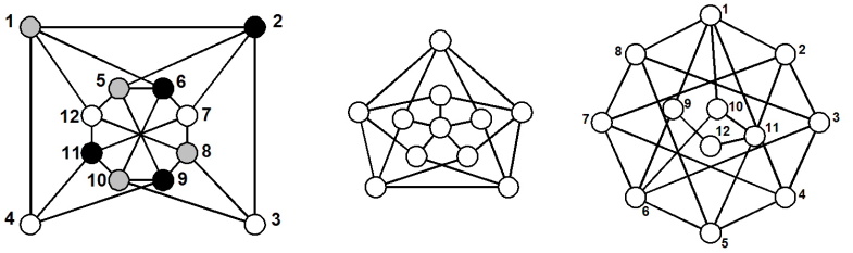
Figure 9: These graphs (from left to right) are (1) a uniquely 3-colorable graph, labeled with its unique 3-coloring [6], (2) the Grötzsch graph, and (3) the Jin graph.

A uniquely 3-colorable graph is a graph that can be colored with three colors in only one way, up to permutation of the color labels. Figure 9 displays a uniquely 3-colorable triangle-free graph [6]. Since the graph is uniquely 3-colorable, the addition of a single edge between two similarly-colored vertices will result in a new non-3-colorable graph. Table 1 also details these experiments. Finally, we investigated all non-3-colorable graphs on six vertices or less: every one has a Nullstellensatz certificate of degree four.

Figure 10: $3,4$ and 5 flowers (left to right). Note that the 3-flower is 3-colorable, whereas the 4 and 5 flowers are non-3-colorable. It is easy to see that only flowers that are multiples of 3 are 3-colorable.

References

- [1] N. Alon, Combinatorial Nullstellensatz, Combin. Prob. and Comput., 8, (1999), 7–29.
- [2] N. Alon and M. Tarsi, Colorings and orientations of graphs, Combinatorica, 12, (1992), 125–134.
- [3] E. Babson, S. Onn and R.R. Thomas, The Hilbert zonotope and a polynomial time algorithm for universal Gröbner bases, Advances in Applied Mathematics, 30, (2003), 529–544.
- [4] D.A. Bayer, “The Division Algorithm and the Hilbert Scheme,” Ph.D. Thesis, Harvard University, (1982).
- [5] S. Buss and T. Pitassi, Good degree bounds on nullstellensatz refutations of the induction principle, IEEE Conference on Computational Complexity, (1996), 233–242.
- [6] C.-Y. Chao and Z. Chen, On uniquely 3-colorable graphs, Discrete Mathematics, 112, (1993), 374–383.
- [7] D. Cox, J. Little and D. O’Shea, “Ideals,Varieties and Algorithms,” Springer Undergraduate Texts in Mathematics, Springer-Verlag, New York, (1992).
- [8] D. Cox, J. Little and D. O’Shea, “Using Algebraic Geometry,” Springer Verlag Graduate Texts in Mathematics, vol. 185, (1998).
- [9] J.A. De Loera, Gröbner bases and graph colorings, Beitrage zur Algebra und Geometrie, 36(1), (1995), 89–96.
- [10] S. Eliahou, An algebraic criterion for a graph to be four-colourable, Aportaciones Matemáticas, Soc. Matemática Mexicana, Notas de Investigacion, 6, (1992), 3–27.
- [11] K.G. Fischer, Symmetric polynomials and Hall’s theorem, Discrete Math, 69(3), (1988), 225–234.
- [12] M. Garey and D. Johnson, “Computers and Intractability: A Guide to the Theory of NP-Completeness,” W.H. Freeman and Company, Copyright 1979 Bell Telephone Laboratories, Incorporated.
- [13] J. Griggs, C. Grinstead and D. Guichard, The number of maximal independent sets in a connected graph , Discrete Mathematics, 68(2-3), (1988), 211–220.
- [14] J. Harant and I. Schiermeyer, On the independence number of a graph in terms of order and size, Discrete Mathematics, 232(1-3), (2001), 131–138.
- [15] C.J. Hillar and T. Windfeldt, “An algebraic characterization of uniquely vertex colorable graphs,” manuscript 2006, see http://www.math.tamu.edu/~chillar/files/uniquegraphcolorings.pdf
- [16] P. Impagliazzo, P. Pudlák and J. Sgall, Lower bounds for polynomial calculus and the Groebner basis algorithm, Computational Complexity, 8, (1999), 127–144.
- [17] G. Jin, Triangle-free four-chromatic graphs, Discrete Mathematics, 145, (1995), 151–170.
- [18] J. Kollar, Sharp effective Nullstellensatz, J. of the AMS, 1(4), (1988), 963–975.
- [19] M. Kreuzer and L. Robbiano, “Computational Commutative Algebra I,” Springer Verlag, Heidelberg, (2000).
- [20] J.B. Lasserre, Polynomials nonnegative on a grid and discrete optimization, Transactions of the AMS, 354(2), (2001), 631–649.
- [21] M. Laurent, Semidefinite representations for finite varieties, Mathematical Programming, 109, (2007), 1–26.
- [22] M. Laurent and F. Rendl, Semidefinite programming and integer programming. In: “Handbook on Discrete Optimization,” K. Aardal, G. Nemhauser, R. Weismantel (eds.), Elsevier B.V., (2005), 393–514.
- [23] S.R. Li and W.W. Li, Independence number of graphs and generators of ideals, Combinatorica, 1, (1981), 55–61.
- [24] L. Lovász, Stable sets and polynomials, Discrete Mathematics, 124, (1994), 137–153.
- [25] L. Lovász, Oberwolfach meeting on Geometric Convex Combinatorics, Mathematisches Forschungsinstitut Oberwolfach, Germany, June 2002.
- [26] S. Margulies, “Combinatorics, Computer Algebra and Complexity: Gröbner Bases and NP-Complete Problems,” UC Davis Ph.D. dissertation, in preparation, (2008).
- [27] Y. Matiyasevich, A criteria for colorability of vertices stated in terms of edge orientations, (in Russian), Discrete Analysis (Novosibirsk), 26, (1974), 65–71.
- [28] Y. Matiyasevich, Some algebraic methods for calculation of the number of colorings of a graph, (in Russian), Zapiski Nauchnykh Seminarov POMI, 293, (2001), 193–205 (available via www.pdmi.ras.ru).
- [29] M. Mnuk, Representing graph properties by polynomial ideals, In V. G. Ganzha, E. W. Mayr, and E. V. Vorozhtsov, editors, “Computer Algebra in Scientific Computing, CASC 2001.” Proceedings of the Fourth International Workshop on Computer Algebra in Scientific Computing, Konstanz, Springer-Verlag, (2001), 431–444.
- [30] S. Onn, Nowhere-zero flow polynomials, Journal of Combinatorial Theory, Series A, 108, (2004), 205–215.
- [31] P. Parrilo, Semidefinite programming relaxations for semialgebraic problems,” Mathematical Programming Ser. B, 96(2), (2003), 293–320.
- [32] P. Parrilo, “An explicit construction of distinguished representations of polynomials nonnegative over finite sets,” IfA Technical Report AUT02-02, (2002).
- [33] W. Schnyder, Planar graphs and poset dimension, Order, 5, (1989), 323–343.
- [34] A. Schrijver, “Theory of Linear and Integer Programming,” Wiley-Interscience Series in Discrete Mathematics and Optimization, John Wiley & Sons, Chichester, West Sussex, England, 1986.
- [35] S.E. Shauger, Results on the Erdös-Gyárfás conjecture in -free graphs, “Proceedings of the Twenty-ninth Southeastern International Conference on Combinatorics Graph Theory and Computing (Boca Raton, FL, 1998).” Congr. Numer., 134, (1998), 61–65.
- [36] A. Simis, W. Vasconcelos and R. Villarreal, On the ideal theory of graphs, J. Algebra, 167(2), (1994), 389–416.
- [37] M. Yannakakis, Expressing combinatorial optimization problems by linear programs, J. Comput. Syst. Sci., 43(3), (1991), 441–466.