Power Spectra of the Total Occupancy in the Totally Asymmetric Simple Exclusion Process

Abstract

As a solvable and broadly applicable model system, the totally asymmetric exclusion process enjoys iconic status in the theory of non-equilibrium phase transitions. Here, we focus on the time dependence of the total number of particles on a 1-dimensional open lattice, and its power spectrum. Using both Monte Carlo simulations and analytic methods, we explore its behavior in different characteristic regimes. In the maximal current phase and on the coexistence line (between high/low density phases), the power spectrum displays algebraic decay, with exponents $-1.62$ and $-2.00$, respectively. Deep within the high/low density phases, we find pronounced oscillations, which damp into power laws. This behavior can be understood in terms of driven biased diffusion with conserved noise in the bulk.

Introduction. The collective behavior of many constituents, interacting under non-equilibrium conditions, is far from well understood. Yet, such systems are ubiquitous in nature, from molecular biology at the nanoscale to infractructure networks at the global level. In physics, attacks on such highly complex systems often begin with seemingly small steps, defining simple models that are both tractable and believed to capture the essentials of the original problem. On this stage, the totally asymmetric simple exclusion process (TASEP) TASEP plays a key role, much like the Ising model in equilibrium statistical mechanics. With open boundaries, particles stochastically enter a one-lane lattice from one end, hop to the next site if it is empty, and leave at the opposite end. This simple transport model provides the first crucial steps towards the modeling of realistic processes, such as protein synthesis, surface growth, and vehicular traffic TASEP-appl . Further, it generates much theoretical interest: Despite its simplicity, its stationary state displays several phases and interesting algebraic correlations, much of which is known analytically TASEP-sol .

In this study, we focus on another simple quantity in TASEP: the total number of particles in the system at time $t$, $N(t)$. In the steady state, its time average should be the ensemble average, which can be easily computed from the known stationary distribution. However, as a fluctuating quantity, its power spectrum, $I(\omega)$, contains time-correlation information which is not as easily accessible. Although such correlations have been investigated recently PPOF , we find interesting behavior undetected previously: oscillatory behavior in $I(\omega)$ for the high and low density phases. While the previous study concerns correlations within the bulk of an infinite system, the new feature here is that our $I\left(\omega\right)$ carries information on the entirety of a finite system. Since many physical systems are far from the thermodynamic limit (e.g., mRNAs containing around $10^{3}$ codons or fewer), such finite-size effects can be physically significant. In the remainder of this letter, we briefly summarize the details of the model, our simulation methods, report our findings, and provide theoretical explanations for the phenomena.

The model and simulation results. A standard TASEP consists of particles hopping on a lattice of length $L$ with site label $i$. If the first site is empty, a particle enters the system with rate $\alpha$. A particle on the last site leaves the system with rate $\beta.$ In the bulk, a particle always hops onto the next site (with unit rate) if the site is empty; otherwise, it remains stationary. A configuration at any particular time is described by a set of occupation numbers $\left\{n_{i}\right\}$ ($n=0,1$ for a vacant vs. occupied site). In all our simulations, we start with an empty lattice and use random sequential updates, i.e., in each Monte Carlo step (MCS), we make $N+1$ random attempts to move a particle. Since the system is stochastic, a complete description requires $P\left(\left\{n_{i}\right\},t\right)$, the probability to find the system in configuration $\left\{n_{i}\right\}$ at time $t$. The evolution of $P$ is governed by a simple master equation. Though linear and typically easy to write, this equation cannot be solved in general. Yet, in the long time limit, $P$ settles into a $t$-independent distribution: $P^{\ast}$, the exact form of which is known TASEP-sol .

The macroscopic properties of these stationary states can be categorized in terms of three distinct phases, conveniently displayed as a phase diagram (Fig. 1a) in the $\alpha$-$\beta$ plane. Thanks to the exact solution, $P^{\ast}$, many properties can be computed analytically. The three regions are associated with the high density (HD), low density (LD), and maximum current (MC) phases. They are distinguished by their average local densities, $\rho_{i}\equiv\left\langle n_{i}/L\right\rangle$, where $\left\langle\bullet\right\rangle$ is an average over the stationary $P^{\ast}\left(\left\{n_{i}\right\}\right)$. In the thermodynamic limit and deep in the bulk, $\rho_{i}$ is $\rho_{+}=1-\beta$, $\rho_{-}=\alpha$, and ${1/2}$ for, respectively, the HD, LD, and MC phases. All aspects of the LD and HD phases can be directly related through particle-hole symmetry, so that we will concentrate only on the LD phase in this letter. For the LD phase, the deviations from $\rho_{-}$ are confined to a microscopic boundary layer near the exit. In the MC phase, the profile decays algebraically into the bulk, while the system displays behavior comparable to critical phenomena in equilibrium statistical mechanics. The transitions at the boundaries of the MC phase are continuous. By contrast, a discontinuity occurs across the HD/LD line. On this line ($\alpha=\beta<1/2$), typical configurations display the coexistence of regions with $\rho_{+}$ and $\rho_{-}$, joined by a microscopically sharp interface, known as a “shock”. The shock is delocalized, performing a random walk over the entire lattice, so that the average $\rho_{i}$ is linear over the interval $\left[\alpha,1-\alpha\right]$.

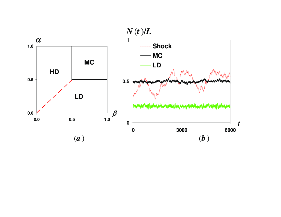
Figure 1: (a) Phase diagram of TASEP. On the dashed line, high and low density domains coexist, with a microscopic interface, known as the “shock.” (b) Typical time series (up to 600K MCS shown) of $N\left(t\right)$, for $L=1000$, in the three distinct regimes: coexistence, MC and LD (color online).

Our main interest here is $N(t)\equiv\sum_{i}n_{i}(t)$ and its associated power spectrum: $I(\omega)$. Though its time average (in the steady state) is just $\sum_{i}\left\langle n_{i}\right\rangle\equiv\bar{\rho}L$, $I(\omega)$ cannot be accessed from $P^{\ast}$. Specifically, we take a measurement of $N$ every 100 MCS (after discarding the first 100K MCS to allow the system to reach steady state) and label these by $t=1,2,...,T$. Typical $N(t)$’s in the three regimes are shown in Fig. 1b. For all but a few of our runs, $T=10^{4}$ ($10^{6}$ MCS), so that we can define a Fourier transform: $\tilde{N}\left(\omega\right)\equiv\sum_{t=1}^{T}N(t)e^{i\omega t}$, where $\omega=2\pi m/T$ with $m=0,1,...$ . To obtain the average power spectrum, we carry out typically 100 such runs and construct

$$I(\omega)=\left\langle\left|\tilde{N}\left(\omega\right)\right|^{2}\right\rangle.$$ (1)

The important control parameters for this system are $L$, $\alpha$, and $\beta$. We investigated a range of $L$’s from $250$ to $32000$. Here, we will show the results for $L=1000$, as well as some for the largest size. Also, we will present mainly data for three representative points in the phase diagram. Labeled by $\left(\alpha,\beta\right)$, they are $\left(0.7,0.7\right)$, $\left(0.3,0.7\right)$, and $\left(0.3,0.3\right)$, corresponding to, respectively, the MC, LD phases and the coexistence line. Systematic studies of the rest of the $\alpha$-$\beta$ square will be reported elsewhere promises .

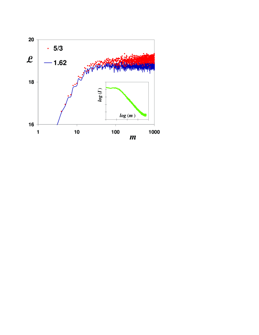
Figure 2: Power spectrum in the MC phase, $\alpha=\beta=0.7$. with $L=1000$. The inset shows a log-log plot of $I\left(\omega\right)$. The main figure shows $\mathcal{L}\equiv\ln\left(\omega^{p}I\right)$ vs. $m\equiv\omega T/2\pi$ (color online).

In the inset of Fig. 2, we show the power spectra for the MC phase. Away from high and low $\omega$ values, $I\left(\omega\right)$ appears to obey a power law: $I\propto\omega^{-p}$. The saturation at small $\omega$ is due to finite $L$ and the crossover scales with the expected $L^{-3/2}$ (see below). At large $\omega$, we are presumably probing an ultraviolet cutoff, due to a discrete lattice and MCS. To expose the power $p$ more effectively, we display $\omega^{p}I$ in a log-log plot (Fig. 2). The best fit seems to be $p=1.62$ (line, blue online), though the data are still consistent with $5/3$ (dots, red online), a value favored by the theoretical considerations below. Whether the difference of $\sim 3\%$ is truly significant remains to be explored promises . We have also simulated other points in the MC phase and find all data to be statistically indistinguishable from the set here. The results for the coexistence line, at $\alpha=\beta=0.3$, are very similar, except that they confirm the expected random walk behavior, with a power of $2$. The most remarkable phenomena are found in the HD/LD phases. As illustrated in Fig. 3, $I\left(\omega\right)$ displays large, damped oscillations. The examples in the inset are especially striking: An $L=32K$ lattice is used here, with three $\alpha$’s. In the next section, we briefly present the theory which accounts for these properties.

Theoretical approaches. To understand the behavior of the power spectra above, we rely on different (though related) approaches for the three regimes. The simplest case is the coexistence line, where the shock performs a random walk. As a result, $N\left(t\right)$ is also just a random walk (Fig. 1b) in the interval $\left[\rho_{-}L,\rho_{+}L\right]$ with reflecting boundary conditions DW . The power spectrum of this process is well understood, displaying the $\omega^{-2}$ behavior. Of course, for small $\omega$ (and long times), $I\left(\omega\right)$ saturates to a finite value, controlled by the allowed interveral for $N$. Later promises , we will show that the expected crossover exhibits data collapse with a scaling variable $\omega L^{2}$. The next regime, considered the most challenging theoretically, is the MC phase. Here, the associated non-equilibrium steady state is “critical”, displaying (power law) correlations and anomalous exponents. At the coarse-grained level, our system is described by a continuous density, $\rho\left(x,t\right)$, and may be studied as a stochastic field theory. Indeed, the TASEP is a driven diffusive system DDS in one dimension. Deviations of $\rho$ about its average here, $\phi\left(x,t\right)\equiv\rho\left(x,t\right)-1/2$, satisfy the noisy Burgers equation Burgers : $\partial_{t}\phi=\frac{1}{2}\partial_{x}^{2}\phi+\partial_{x}\phi^{2}+\partial_{x}\eta$, where $\eta$ is a Gaussian noise. Within the bulk of an infinite system, the dynamic two-point function $\left\langle\phi\left(x,t\right)\phi\left(x^{\prime},t^{\prime}\right)\right\rangle$ is translationally invariant and assumes a scaling form PPOF ; DDS ; FNS :

$$C\left(\xi,\tau\right)=\xi^{-1}f\left(\xi/\tau^{2/3}\right)$$ (2)

where $\xi=x^{\prime}-x$ and $\tau=t^{\prime}-t$. If we naively consider $\int d\xi C\left(\xi,\tau\right)$ as a candidate for our power spectrum, we would find that Eqn. (2) leads to $\int dsf\left(s\right)$, independent of $\tau$! This surprising conlusion is consistent with simply setting $k=0$ in the results of JS . On closer examination, however, we should seek the Fourier transform of $\int_{0}^{L}dxdx^{\prime}\left\langle\phi\left(x,0\right)\phi\left(x^{\prime},t\right)\right\rangle$ in a finite system. If we approximate this two-point function by $C\left(\xi,\tau\right)$, we are led to $\int_{0}^{L}d\xi\left[2\left(L-\xi\right)C\left(\xi,t\right)\right]$, which is of the form $t^{2/3}g\left(L/t^{2/3}\right)$. Thus, its Fourier transform would take the scaling form $I\left(\omega\right)=\omega^{-5/3}G\left(L\omega^{2/3}\right)$. Assuming that $G$ approaches a positive constant for $\omega\gg L^{-3/2}$, this theory predicts $I\left(\omega\right)\propto\omega^{-5/3}$. As discussed above, our data are consistent with this power, although $1.62$ appears to be a better fit. Though a 3% disagreement seems minor, we found similar discrepancies in other observables such as $\left\langle N\left(t\right)N\left(t^{\prime}\right)\right\rangle$. These issues, along with finite-size corrections to scaling, discrete space and time, and possible systematic errors, will be explored elsewhere promises .

Figure 3: Power spectrum $I\left(\omega\right)$ vs. $m\equiv\omega T/2\pi$ in the LD phase ($\alpha=1-\beta=0.3$) with $L=1000$. The inset shows a similar plot for a $L=32000$ lattice, with $\alpha=1-\beta=0.2,\,0.3,\,$ and $0.4$. The units for $log\left(I\right)$ are arbitrary, and the curves are displaced for clarity (color online).

Typically, the behavior deep in the HD and LD phases seems least interesting, with ordinary Gaussian fluctuations. Yet, $I\left(\omega\right)$ for this regime exhibits the most structure. We now turn to a brief account of a simple, linear theory for the fluctuations that predicts these interesting oscillations, focusing on the LD phase only.

Following standard routes for a continuum description DDS ; PPOF of a driven density $\rho(x,t)$, we study small fluctuations, $\phi$, around $\bar{\rho}$ using the stochastic equation of motion: $\partial_{t}\phi(x,t)=D\partial_{x}^{2}\phi-v\partial_{x}\phi+\partial_{x}\eta$. Here, $D$ is the (effective) diffusion constant, $v$ is the bias, and $\eta$ is a Gaussian correlated (local) noise with zero mean. If we were to start from the microscopic $\left\{n_{i}\right\}$ and take a naive continuum limit, we would arrive at $D=1/2$ and $v=1-2\bar{\rho}$ (in units of lattice spacing and MCS). But we leave these as $O\left(1\right)$ parameters for now. The solution in Fourier space is easy: $\tilde{\phi}\left(k,\omega\right)=ik\tilde{\eta}\left(k,\omega\right)/\left[Dk^{2}+ivk-i\omega\right]$, where $\phi(x,t)=\int_{k,\omega}\tilde{\phi}\left(k,\omega\right)e^{i(kx-\omega t)}$ and $\int_{k}\equiv\int dk/2\pi$. With $N\left(t\right)=\int_{0}^{L}dx\rho\left(x,t\right)=\bar{\rho}L+\int_{0}^{L}\phi\left(x,t\right)$, we have $\tilde{N}\left(\omega\right)=\int_{k}\left(e^{ikL}-1\right)\tilde{\eta}/\left[Dk^{2}+ivk-i\omega\right]$ for $\omega>0$. Writing $\left\langle\tilde{\eta}\left(k,\omega\right)\tilde{\eta}^{\ast}\left(k^{\prime},\omega^{\prime}\right)\right\rangle=A\delta\left(k-k^{\prime}\right)\delta\left(\omega-\omega^{\prime}\right)$ and replacing $\delta\left(\omega-\omega\right)$ by $T$, we find the power spectrum to be $\frac{AT}{2\pi}\int_{k}\left|\left(e^{ikL}-1\right)/\left[Dk^{2}+ivk-i\omega\right]\right|^{2}$. Evaluting the integral, we arrive at

$$I\left(\omega\right)=\frac{8ADT}{v^{3}}\mathop{\rm Re}\left[\frac{e^{ik_{+}L}-1}{R\left(1-R\right)^{2}}+\frac{e^{ik_{-}^{*}L}-1}{R^{*}\left(1+R^{*}\right)^{2}}\right]$$ (3)

where $R\equiv\sqrt{1-4iD\omega/v^{2}}$ and $k_{\pm}=iv\left(-1\pm R\right)/2D$.

To shed light on this complex expression, we consider three frequency regimes: (a) $\omega\rightarrow 0$, e.g., $m=1,2,3...$, (b) intermediate $\omega$’s ($\omega\ll v^{2}/D$, i.e., $1\ll m\ll T$), and (c) $\omega\rightarrow\infty$. In regime (a), $I$ approaches a constant, which can be used to fit $A$. A further simplication is that the first term in $\mathop{\rm Re}\left[...\right]$ is $O\left(\left(vL/D\right)^{2}\right)$, while the second term is $O\left(1\right)$. Thus, the latter can be largely ignored, if we take, e.g., $L=32K$, as in the inset of Fig. 3. In regime (b), we keep $O\left(\omega^{2}\right)$ corrections in $R$ and $k_{\pm}$, i.e.,

$$1-\frac{2iD\omega}{v^{2}}+\frac{2D^{2}\omega^{2}}{v^{4}}\quad\text{and}\quad\frac{\omega}{v}+\frac{iD\omega^{2}}{v^{3}}$$

respectively. The result shows damped oscillations manifestly:

$$I\left(\omega\right)\cong\frac{2AvT}{D\omega^{2}}\left[1-e^{-\frac{D\omega^{2}L}{v^{3}}}\cos\left(\omega L/v\right)\right].$$ (4)

The minima are near integer multiples of $2\pi v/L$ in $\omega$ (i.e., $vT/L$ in $m$). Remarkably, the minima in Fig. 3 are very close to these values if we naively substitute $\left(0.4,10^{6},10^{3}\right)$ for $\left(v,T,L\right)$. Encouraged by this approach, we attempt to fit the $L=32K$ data with the full Eqn. (3). The result for $\alpha=0.3$, shown in Fig. 4, is surpringly good, indicating that this simple theory has captured the essentials of our system.

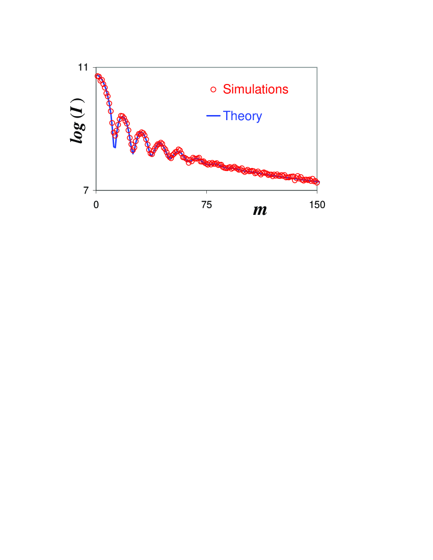
Figure 4: Power spectrum $\log\left(I\right)$ vs. $m$ for $\alpha=1-\beta=0.3$ with $L=32000$ (color online).

The physical origins of the oscillations are noteworthy. They can be traced to the time it takes a fluctuation to traverse the entire lattice. Indeed, if there is no exclusion and each particle travels ballistically at velocity $u$, then $N\left(t\right)$ will consist of a random series of unit increments (due to $\alpha$), correlated with unit drops at times $L/u$ later (assuming $\beta=1$). The associated $I$ will be proportional to $z^{-2}\sin^{2}z$, with $z\equiv\omega L/2u$, with zeros at multiples of $2\pi u/L$. The effect of diffusion, embodied in $D$, is just to smear out the minima and fill in the zeros. Returning to the fit above, we were surprised that it requires $D\simeq 20$ and $A\simeq 1/500$, values that seem remarkably far from the naive $O\left(1\right)$ levels. Work is in progress to understand why these parameters are so seriously “renormalized.”promises

Beyond the oscillations, there is another subtle feature in this intermediate $\omega$ regime. As Eqn. (4) shows, the oscillations are completely damped when $\omega^{2}$ exceeds $v^{3}/DL$, and $I$ settles into $\omega^{-2}$. Though not shown, this power is confirmed in the $L=32K$ case. However, on further scrutiny, we see that $R\rightarrow\sqrt{\omega}$ in the truly asymptotic regime (c): $\omega\gg v^{2}/4D$. Then, Eqn. (3) predicts a $\omega^{-3/2}$ decay 3/2 power ! If this regime is reached before the oscillations are fully damped, then the $\omega^{-2}$ behavior of the “intermediate regime” will lie hidden. This is indeed true for the $L=1K$ case, where the oscillations die out at much larger $m$’s and only the $3/2$ power is observed.

Outlook. In addition to a more detailed and systematic Monte Carlo study (e.g., larger systems, longer runs, finite-size scaling, etc.), there are a number of issues worthy of further pursuit. The continuum theory represents a rough first step and should be refined to a version with discrete space/time. Most intimately connected to this work is a better understanding of the origin of the large “renormalization effects” on the diffusion coefficient, $D$. Beyond interests specific to the simple TASEP, we are motivated by its applicability to protein synthesis, where the lattice (particles) model the mRNA (ribosomes) TASEP-appl . To capture more of the process in vivo, we should include the effects of (i) particles that occupy $\ell>1$ sites, (ii) inhomogeneous hopping rates, (iii) finite reservoir of particles which can enter the lattice, and (iv) competition with other TASEPs (mRNAs) for a finite pool of particles. Some of these issues have been considered TASEP-appl , though none focused on the total occupancy, a quantity surely of interest in the context of biology. Needless to say, many other generalizations - all well motivated by physical systems - come to mind, e.g., many particle species, multiple lanes, and high dimensions. In the past, power spectra have served us well, providing valuable perspectives into stochastic systems in general PSpGenRef and driven system in particular PSpDDS . We hope this work will spark further interest to study power spectra in novel non-equilibrium systems far beyond physics, such as biology, social networks, and finance.

References

- (1) F. Spitzer, Adv. Math. 5, 246 (1970). For a recent review, see G. Schütz, Exactly solvable models in many-body systems, Vol. 19 of Phase Transition and Critical Phenomena, eds C. Domb and J.L. Lebowitz (Academic, London, 2001).
- (2) C. MacDonald, J. Gibbs, and A. Pipkin, Biopolymers, 6, 1 (1968); C. MacDonald and J. Gibbs, Biopolymers, 7, 707 (1969); D.E. Wolf, and L.-H. Tang, Phys. Rev. Lett. 65, 1591 (1990); V. Popkov, L. Santen, A. Schadschneider, and G.M. Schütz, J. Phys. A: Math. Gen. 34, L45 (2001); L.B. Shaw, R.K.P. Zia, and K.H. Lee, Phys. Rev. E 68, 021910 (2003); T. Chou and G. Lakatos, Phys. Rev. Lett. 93, 198101 (2004).
- (3) See, e.g., B. Derrida, Phys. Rep. 301, 65 (1998) and the review in TASEP .
- (4) P. Pierobon, A. Parmeggiani, F. von Oppen, and E. Frey, Phys. Rev. E 72, 036123 (2005). Note that the power spectrum considered in this reference (Eqn. 26) is associated with the autocorrelation of the local density fluctuations. It should be distinguished from our correlation of the total occupation in the system.
- (5) D.A. Adams, B. Schmittmann, and R.K.P. Zia, to be published.
- (6) B. Derrida, E. Domany, and D. Mukamel, J. Stat. Phys. 69, 667 (1992). L. Santen + C. Appert J. Stat. Phys. 106, 187 (2002).
- (7) H.K. Janssen and B. Schmittmann, Z. Phys. B63, 517 (1986); For a general review, see B. Schmittmann and R.K.P. Zia Statistical Mechanics of Driven Diffusive Systems, Vol. 17 of Phase Transitions and Critical Phenomena, eds C. Domb and J.L. Lebowitz (Academic, New York, 1995).
- (8) J.M. Burgers, The Nonlinear Diffusion Equation (Riedel, Boston, 1974).
- (9) D. Forster, D.R. Nelson, and M.J. Stephen, Phys. Rev. A16, 732 (1977).
- (10) Specifically, see Eqns. (21b) and (24a) in DDS and also FNS and H. van Beijeren, R. Kutner, and H. Spohn, Phys. Rev. Lett. 54, 2026 (1985).
- (11) We emphasize that, despite the similarity, this is not the same as in PPOF , which focused on the power spectrum of the local density fluctuations.
- (12) See, e.g., H. L. Pecseli, Fluctuations in Physical Systems (Cambridge, UK, 2000).
- (13) See, e.g., J.V. Andersen, H.K. Jensen, and O.G. Mouritsen, Phys. Rev. B44, 439 (1991); K-t. Leung, Phys. Rev. B44, 5340 (1991); K.B. Lauritsen and H.C. Fogedby, J. Stat. Phys. 72, 189 (1993).