TROPICAL IMPLICITIZATION
AND MIXED FIBER POLYTOPES

Abstract

The software TrIm offers implementations of tropical implicitization and tropical elimination, as developed by Tevelev and the authors. Given a polynomial map with generic coefficients, TrIm computes the tropical variety of the image. When the image is a hypersurface, the output is the Newton polytope of the defining polynomial. TrIm can thus be used to compute mixed fiber polytopes, including secondary polytopes.

14Q10, 52B20, 52B55, 65D18

1 Introduction

Implicitization is the problem of transforming a given parametric representation of an algebraic variety into its implicit representation as the zero set of polynomials. Most algorithms for elimination and implicitization are based on multivariate resultants or Gröbner bases, but current implementations of these methods are often too slow. When the variety is a hypersurface, the coefficients of the implicit equation can also be computed by way of numerical linear algebra [3, 7], provided the Newton polytope of that implicit equation can be predicted a priori.

The problem of predicting the Newton polytope was recently solved independently by three sets of authors, namely, by Emiris, Konaxis and Palios [8], Esterov and Khovanskii [13], and in our joint papers with Tevelev [18, 19]. A main conclusion of these papers can be summarized as follows: The Newton polytope of the implicit equation is a mixed fiber polytope.

The first objective of the present article is to explain this conclusion and to present the software package TrIm for computing such mixed fiber polytopes. The name of our program stands for Tropical Implicitization, and it underlines our view that the prediction of Newton polytopes is best understood within the larger context of tropical algebraic geometry. The general theory of tropical elimination developed in [18] unifies earlier results on discriminants [4] and on generic polynomial maps whose images can have any codimension [19]. The second objective of this article is to explain the main results of tropical elimination theory and their implementation in TrIm. Numerous hands-on examples will illustrate the use of the software. At various places we give precise pointers to [8] and [13], so as to highlight similarities and differences among the different approaches to the subject.

Our presentation is organized as follows. In Section 2 we start out with a quick guide to TrIm by showing some simple computations. In Section 3 we explain mixed fiber polytopes. That exposition is self-contained and may be of independent interest to combinatorialists. In Section 4 we discuss the computation of mixed fiber polytopes in the context of elimination theory, and in Section 5 we show how the tropical implicitization problem is solved in TrIm. Theorem 5.1 expresses the Newton polytope of the implicit equation as a mixed fiber polytope. In Section 6 we present results in tropical geometry on which the development of TrIm is based, and we explain various details concerning our algorithms and their implementation.

2 How to use TrIm

The first step is to download TrIm from the following website which contains information for installation in Linux:

http://math.mit.edu/~jyu/TrIm

TrIm is a collection of C++ programs which are glued together and integrated with the external software polymake [9] using perl scripts. The language perl was chosen for ease of interfacing between various programs.

The fundamental problem in tropical implicitization is to compute the Newton polytope of a hypersurface which is parametrized by Laurent polynomials with sufficiently generic coefficients. As an example we consider the following three Laurent polynomials in two unknowns $x$ and $y$ with sufficiently generic coefficients $\alpha_{1},\alpha_{2},\alpha_{3},\beta_{1},\beta_{2},\beta_{3},\gamma_{1},\gamma_{2},\gamma_{3}$:

$$u\quad = \quad\alpha_{1}\cdot\frac{1}{x^{2}y^{2}}\,+\,\alpha_{2}\cdot x\,+\,\alpha_{3}\cdot xy$$

$$v\quad = \quad\beta_{1}\cdot x^{2}\,+\,\beta_{2}\cdot y\,+\,\beta_{3}\cdot\frac{1}{x}$$

$$w\quad = \quad\gamma_{1}\cdot y^{2}\,+\,\gamma_{2}\cdot\frac{1}{xy}\,+\,\gamma_{3}\cdot\frac{1}{y}.$$

We seek the unique (up to scaling) irreducible polynomial $F(u,v,w)$ which vanishes on the image of the corresponding morphism $(\mathbb{C}^{*})^{2}\rightarrow\mathbb{C}^{3}$. Using our software TrIm, the Newton polytope of the polynomial $F(u,v,w)$ can be computed as follows. We first create a file input with the contents

[x,y]
[x^(-2)*y^(-2) + x + x*y,
 x^2 + y + x^(-1),
 y^2 + x^(-1)*y^(-1) + y^(-1)]

Here the coefficients are suppressed: they are tacitly assumed to be generic. We next run a perl script using the command ./TrIm.prl input. The output produced by this program call is quite long. It includes the lines

VERTICES
1  9 2 0
1  0 9 2
1  0 9 0
1  0 0 9
1  6 6 0
1  2 2 8
1  0 6 6
1  2 8 2
1  6 0 6
1  0 0 0
1  9 0 0
1  2 0 9
1  8 2 2

Ignoring the initial 1, this list consists of $13$ lattice points in $\mathbb{R}^{3}$, and these are precisely the vertices of the Newton polytope of $F(u,v,w)$. The above output format is compatible with the polyhedral software Polymake [9]. We find that the Newton polytope has $10$ facets, $21$ edges, and $13$ vertices. Further down in the output, TrIm prints a list of all lattice points in the Newton polytope, and it ends by telling us the number of lattice points:

N_LATTICE_POINTS
383

Each of the $383$ lattice points $(i,j,k)$ represents a monomial $u^{i}v^{j}w^{k}$ which might occur with non-zero coefficient in the expansion of $F(u,v,w)$. Hence, to recover the coefficients of $F(u,v,w)$ we must solve a linear system of $382$ equations with $383$ unknowns. Interestingly, in this example, $39$ of the $383$ monomials always have coefficient zero in $F(u,v,w)$. Even when $\alpha_{1},\ldots,\gamma_{3}$ are completely generic, the number of monomials in $F(u,v,w)$ is only $344$.

The command ./Trim.prl implements a certain algorithm, to be described in the next sections, whose input consists of $n$ lattice polytopes in $\mathbb{R}^{n-1}$ and whose output consists of one lattice polytope in $\mathbb{R}^{n}$. In our example, with $n=3$, the input consists of three triangles and the output consisted of a three-dimensional polytope. These are depicted in Figure 1.

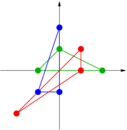
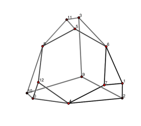
Input	Output

Figure 1: Tropical implicitization constructs the three-dimensional Newton polytope of a parametrized surface from the three Newton polygons of the given parametrization

The program also works in higher dimensions but the running time quickly increases. For instance, consider the hypersurface in $\mathbb{C}^{4}$ represented by the following four Laurent polynomials in $x,y,z$, written in TrIm format:

[x,y,z]
[x*y + z + 1,
 x*z + y + 1,
 y*z + x + 1,
 x^3 + y^5 + z^7]

It takes ${\tt TrIm}$ a few moments to inform us that the Newton polytope of this hypersurface has $40$ vertices and contains precisely $5026$ lattice points. The $f$-vector of this four-dimensional polytope equals $(40,111,103,32)$.

Remark 2.1.

The examples above may serve as illustrations for the results in the papers [8] and [13]. Emiris, Konaxis and Palios [8] place the emphasis on computational complexity, they present a precise formula for plane parametric curves, and they allow for the map to given by rational functions. Esterov and Khovanskii develop a general theory of polyhedral elimination, which parallels the tropical approach in [18], and which includes implicitization as a very special case. A formula for the leading coefficients of the implicit equation is given in [8, §4]. This formula is currently not implemented in TrIm but it could be added in a future version.

What distinguishes TrIm from the approaches in [8] and [13] is the command TrCI which computes the tropical variety of a generic complete intersection. The relevant mathematics will be reviewed in Section 6. This command is one of the ingredients in the implementation of tropical implicitization. The input again consists of $m$ Laurent polynomials in $n$ variables whose coefficients are tacitly assumed to be generic, or, equivalently, of $m$ lattice polytopes in $n$-space. Here it is assumed that $m\leq n$. If equality holds then the program simply computes the mixed volume of the given polytopes. As an example, delete the last line from the previous input file:

[x,y,z]
[x*y + z + 1,
 x*z + y + 1,
 y*z + x + 1]

The command ./TrCI.prl input computes the mixed volume of the three given lattice polytopes in $\mathbb{R}^{3}$. Here the given polytopes are triangles. The last line in the output shows that their mixed volume equals five.

Now repeat the experiment with the input file input as follows:

[x,y,z]
[x*y + z + 1,  x*z + y + 1]

The output is a one-dimensional tropical variety given by five rays in $\mathbb{R}^{3}$:

DIM
1

RAYS
 0 -1 -1
 0  0  1
 1  0  0
 0  1  0
-1  1  1

MAXIMAL_CONES
0
1
2
3
4

MULTIPLICITIES
2
1
1
1
1

Note that the first ray, here indexed by 0, has multiplicity two. This scaling ensures that the sum of the five RAYS equals the zero vector $(0,0,0)$.

For a more interesting example, let us tropicalize the complete intersection of two generic hypersurfaces in $\mathbb{C}^{5}$. We prepare input as follows:

[a,b,c,d,e]
[a*b + b*c + c*d + d*e + a*e + 1,
 a*b*c + b*c*d + c*d*e + d*e*a + e*a*b]

When applied to these two polynomials in five unknowns, the command ./TrCI.prl input produces a three-dimensional fan in $\mathbb{R}^{5}$. This fan has $26$ rays and it has $60$ maximal cones. Each maximal cone is the cone over a triangle or a quadrangle, and it has multiplicity one. The rays are

RAYS
-1  1  0  0  1
-1  1  1 -1  3
 0  1  0  0  1
-1  3 -1  1  1

$\,\,\,\cdots\quad\cdots\quad\cdots$

The rays are labeled $0,1,\ldots,25$, in the order in which they were printed. The maximal (three-dimensional) cones appear output in the format

MAXIMAL_CONES
0 1 2 3
0 1 7 10
0 1 12
0 3 4 7
0 3 12
0 7 12

$\,\cdots\,\,\,\cdots$

It is instructive to compute the tropical intersection of two generic hypersurfaces with the same support. For example, consider the input file

[x,y,z]
[1 + x + y + z + x*y + x*z + y*z + x*y*z,
 1 + x + y + z + x*y + x*z + y*z + x*y*z]

As before, the reader should imagine that the coefficients are generic rational numbers instead of one’s. The tropical complete intersection determined by these two equations consists of the six rays normal to the six facets of the given three-dimensional cube. The same output would be produced by Jensen’s software GFan [2, 12], which computes arbitrary tropical varieties, provided we input the two equations with generic coefficients.

3 Mixed fiber polytopes

We now describe the construction of mixed fiber polytopes. These generalize ordinary fiber polytopes [1], and hence they generalize secondary polytopes [10]. The existence of mixed fiber polytopes was predicted by McDonald [14] and Michiels and Cools [16] in the context of polynomial systems solving. They were first constructed by McMullen [15], and later independently by Esterov and Khovanskii [13].

The presentation in this section is written entirely in the language of combinatorial geometry, and it should be of independent interest to some of the readers of Ziegler’s text book [20]. There are no polynomials or varieties in this section, neither classical nor tropical. The connection to elimination and tropical geometry will be explained in subsequent sections.

Consider a linear map $\,\pi:\mathbb{R}^{p}\rightarrow\mathbb{R}^{q}$ and a $p$-dimensional polytope $P\subset\mathbb{R}^{p}$ whose image $Q=\pi(P)$ is a $q$-dimensional polytope in $\mathbb{R}^{q}$. If $x$ is any point in the interior of $Q$ then its fiber $\,\pi^{-1}(x)\cap P\,$ is a polytope of dimension $p-q$. The fiber polytope is defined as the Minkowski integral

$$\Sigma_{\pi}(P)\quad=\quad\int_{Q}(\pi^{-1}(x)\cap P)\,dx.$$ (1)

It was shown in [1] that this integral defines a polytope of dimension $p-q$. The fiber polytope $\Sigma_{\pi}(P)$ lies in an affine subspace of $\mathbb{R}^{p}$ which is a parallel translate of $\,{\rm kernel}(\pi)$. Billera and Sturmfels [1] used the notation $\Sigma(P,Q)$ for the fiber polytope, and they showed that its faces are in bijection with the coherent polyhedral subdivisions of $Q$ which are induced from the boundary of $P$. We here prefer the notation $\Sigma_{\pi}(P)$ over the notation $\Sigma(P,Q)$, so as to highlight the dependence on $\pi$ for fixed $P$ and varying $\pi$.

Example 3.1

Let $p=3$ and take $P$ to be the standard $3$-cube

$$P\,\,\,=\,\,\,{\rm conv}\bigl{\{}(000),(001),(010),(011),(100),(101),(110),(111)\bigr{\}}.$$

We also set $q=1$ and we fix the linear map

$$\pi:\mathbb{R}^{3}\rightarrow\mathbb{R}^{1},\,(u,v,w)\mapsto u+2v+3w.$$

Then $Q=\pi(P)$ is the line segment $[0,6]$. For $0<x<6$, each fiber $\pi^{-1}(x)\cap P$ is either a triangle, a quadrangle or a pentagon. Since the fibers have a fixed normal fan over each open segment $(i,i+1)$, we find

$$\Sigma_{\pi}(P)\quad=\quad\sum_{i=0}^{5}\int_{i}^{i+1}\!(\pi^{-1}(x)\cap P)\,dx\quad=\quad\sum_{i=0}^{5}\bigl{(}\pi^{-1}(i+\frac{1}{2})\cap P\bigr{)}.$$

Hence the fiber polygon is really just the Minkowski sum of two triangles, two quadrangles and two pentagon, and this turns out to be a hexagon:

$$\Sigma_{\pi}(P)\,\,=\,\,{\rm conv}\bigl{\{}(1,10,5),(1,4,9),(5,2,9),(11,2,7),(11,8,3),(7,10,3)\bigr{\}}.$$

In the next section we shall demonstrate how TrIm can be used to compute fiber polytopes. The output produced will be the planar hexagon which is gotten from the coordinates above by applying the linear map $(u,v,w)\mapsto(w-3,v+w-9)$. Hence TrIm produces the following coordinatization:

$$\Sigma_{\pi}(P)\,\,\,=\,\,\,{\rm conv}\bigl{\{}(2,6),\,(6,4),\,(6,2),\,(4,0),\,(0,2),\,(0,4)\,\bigr{\}}.$$ (2)

It is no big news to polytope aficionados that the fiber polygon of the $3$-cube is a hexagon. Indeed, by [20, Example 9.8], the fiber polytope obtained by projecting the $p$-dimensional cube onto a line is the permutohedron of dimension $p-1$. For $p=3$ the vertices of the hexagon $\Sigma_{\pi}(P)$ correspond to the six monotone edge paths on the $3$-cube from $(000)$ to $(111)$. ∎

As a special case of the construction of fiber polytopes we get the secondary polytopes. Suppose that $P$ is a polytope with $n$ vertices in $\mathbb{R}^{p}$ and let $\Delta$ denote the standard $(n-1)$-simplex in $\mathbb{R}^{n}$. There exists a linear map $\,\rho:\mathbb{R}^{n}\rightarrow\mathbb{R}^{p}$ such that $\rho(\Delta)=P$, and this linear map is unique if we prescribe a bijection from the vertices of $\Delta$ onto the vertices of $P$. The polytope $\Sigma_{\rho}(\Delta)$ is called the secondary polytope of $P$; see [20, Definition 9.9]. Secondary polytopes were first introduced in an algebraic context by Gel’fand, Kapranov and Zelevinsky [10]. For example, if we take $P$ to be the $3$-dimensional cube as above, then the simplex $\Delta$ is $7$-dimensional, and the secondary polytope $\Sigma_{\rho}(\Delta)$ is a $4$-dimensional polytope with $74$ vertices. These vertices are in bijection with the $74$ triangulations of the $3$-cube.

A detailed introduction to triangulations and a range of methods for computing secondary polytopes can be found in the forthcoming book [5]. We note that the computation of fiber polytopes can in principle be reduced to the computation of secondary polytopes, by means of the formula

$$\Sigma_{\pi}(\rho(\Delta))\,\,\,=\,\,\,\rho(\Sigma_{\pi\circ\rho}(\Delta)).$$ (3)

Here $\pi\circ\rho$ is the composition of the following two linear maps of polytopes:

$$\Delta\stackrel{{\scriptstyle\rho}}{{\longrightarrow}}P\stackrel{{\scriptstyle\pi}}{{\longrightarrow}}Q$$

The formula (3) appears in [1, Lemma 2.3] and in [20, Exercise 9.6]. The algorithm of Emiris et al. [8, §4] for computing Newton polytopes of specialized resultants is based on a variant of (3). Neither our software TrIm nor the Esterov-Khovanskii construction [13] uses the formula (3).

We now come to the main point of this section, namely, the construction of mixed fiber polytopes. This is primarily due to McMullen [15], but was rediscovered in the context of elimination theory by Khovanskii and Esterov [13, §3]. We fix a linear map $\pi:\mathbb{R}^{p}\rightarrow\mathbb{R}^{q}$ as above, but we now consider a collection of $c$ polytopes $P_{1},\ldots,P_{c}$ in $\mathbb{R}^{p}$. We consider the Minkowski sum $\,P_{\lambda}=\lambda_{1}P_{1}+\cdots+\lambda_{c}P_{c}\,$ where $\,\lambda=(\lambda_{1},\ldots,\lambda_{c})$ is a parameter vector of unspecified positive real numbers. We shall assume that $P_{\lambda}$ is of full dimension $p$, but we do allow its summands $P_{i}$ to be lower-dimensional. The image of $P_{\lambda}$ under the map $\pi$ is the $q$-dimensional polytope

$$\pi(P_{\lambda})\,\,\,=\,\,\,\lambda_{1}\cdot\pi(P_{1})+\cdots+\lambda_{c}\cdot\pi(P_{c}).$$

The following result concerns the fiber polytope from $\,P_{\lambda}\,$ onto $\,\pi(P_{\lambda})$.

Theorem 3.2 ([15, 13]).

The fiber polytope $\Sigma_{\pi}(P_{\lambda})$ depends polynomially on the parameter vector $\lambda$. This polynomial is homogeneous of degree $q+1$. Moreover, there exist unique polytopes $\,M_{i_{1}i_{2}\cdots i_{c}}\,$ such that

$$\Sigma_{\pi}(\,\lambda_{1}P_{1}+\cdots+\lambda_{c}P_{c}\,)\,\,\,\,\,=\sum_{i_{1}+\cdots+i_{c}=q+1}\!\!\!\!\!\!\!\lambda_{1}^{i_{1}}\lambda_{2}^{i_{2}}\cdots\lambda_{c}^{i_{c}}\cdot M_{i_{1}i_{2}\cdots i_{c}}.$$ (4)

To appreciate this theorem, it helps to begin with the case $c=1$. That corresponds to scaling the polytopes $P$ and $Q$ above by the same factor $\lambda$. This results in the Minkowski integral (1) being scaled by the factor $\lambda^{q+1}$. More generally, the coefficients of the pure powers $\lambda_{j}^{q+1}$ in the expansion (4) are precisely the fiber polytopes of the individual $P_{j}$, that is,

$$M_{0,\ldots,0,q+1,0,\ldots,0}\,\,=\,\,\Sigma_{\pi}(P_{j}).$$

On the other extreme, we may consider $\,i_{1}=i_{2}=\cdots=i_{c}=1$, which is the term of interest for elimination theory. Of course, if all $i_{j}$’s are equal to one then the number $c$ of polytopes $P_{j}$ is one more than the dimension $q$ of the image of $\pi$. We now assume that this holds, i.e., we assume that $\,c=q+1$. We define the mixed fiber polytope to be the coefficient of the monomial $\lambda_{1}\lambda_{2}\cdots\lambda_{c}$ in the formula (4). The mixed fiber polytope is denoted

$$\Sigma_{\pi}(P_{1},P_{2},\ldots,P_{c})\quad:=\quad M_{11\cdots 1}.$$ (5)

The smallest non-trivial case arises when $p=3$, $c=2$ and $q=1$, where we are projecting two polytopes $P_{1}$ and $P_{2}$ in $\mathbb{R}^{3}$. Their mixed fiber polytope with respect to a linear form $\,\pi:\mathbb{R}^{3}\rightarrow\mathbb{R}^{1}\,$ is the coefficient of $\,\lambda_{1}\lambda_{2}\,$ in

$$\Sigma_{\pi}(\lambda_{1}P_{1}+\lambda_{2}P_{2})\quad=\quad\lambda_{1}^{2}\cdot\Sigma_{\pi}(P_{1})\,\,+\,\,\lambda_{1}\lambda_{2}\cdot\Sigma_{\pi}(P_{1},P_{2})\,\,+\,\,\lambda_{2}^{2}\cdot\Sigma_{\pi}(P_{2}).$$

The following is [18, Example 4.10]. It will be revisited in Example 4.2.

Example 3.3

Consider the following two tetrahedra in three-space:

$$\,P_{1}={\rm conv}\{0,3e_{1},3e_{2},3e_{3}\}\,\hbox{ and }\,P_{2}={\rm conv}\{0,-2e_{1},-2e_{2},-2e_{3}\}.$$

Their Minkowski sum $P_{1}+P_{2}$ has $12$ vertices, $24$ edges and $14$ facets. If we take $\pi:\mathbb{R}^{3}\rightarrow\mathbb{R}^{1}$ to be the linear form $\,(u,v,w)\mapsto u-2v+w\,$ then the fiber polytope $\,\Sigma_{\pi}(P_{1}+P_{2})\,=\,M_{20}\,+\,M_{11}\,+\,M_{02}\,$ is a polygon with ten vertices. Its summands $M_{20}=\Sigma_{\pi}(P_{1})$ and $M_{02}=\Sigma_{\pi}(P_{2})$ are quadrangles, while the mixed fiber polytope $\,M_{11}=\Sigma_{\pi}(P_{1},P_{2})\,$ is a hexagon. ∎

We remark that fiber polytopes are special instances of mixed fiber polytopes. Suppose that $P_{1}=P_{2}=\cdots=P_{c}$ are all equal to the same fixed polytope $P$ in $\mathbb{R}^{p}$. Then the fiber polytope $\Sigma_{\pi}(P_{\lambda})$ in (4) equals

$$\Sigma(\lambda_{1}P_{1}+\cdots+\lambda_{c}P_{c})\quad=\quad(\lambda_{1}+\cdots+\lambda_{c})^{c}\cdot\Sigma_{\pi}(P).$$

Hence the fiber polytope $\Sigma_{\pi}(P)$ is the mixed fiber polytope $\Sigma_{\pi}(P,\ldots,P)$ scaled by a factor of $1/c!$. Similarly, any of the coefficients in the expansion (4) can be expressed as mixed fiber polytopes. Up to scaling, we have

$$\,M_{i_{1}i_{2}\cdots i_{c}}\quad=\quad\,\,\Sigma_{\pi}\bigl{(}\underbrace{P_{1},\ldots,P_{1}}_{i_{1}\,{\rm times}},\underbrace{P_{2},\ldots,P_{2}}_{i_{2}\,{\rm times}},\ldots,\underbrace{P_{c},\ldots,P_{c}}_{i_{c}\,{\rm times}}\bigr{)}.$$

In the next section we shall explain how mixed fiber polytopes, and hence also fiber polytopes and secondary polytopes, can be computed using TrIm.

4 Elimination

Let $\,f_{1},f_{2},\ldots,f_{c}\in\mathbb{C}[x_{1}^{\pm 1},x_{2}^{\pm 1},\ldots,x_{p}^{\pm 1}]\,$ be Laurent polynomials whose Newton polytopes are $P_{1},P_{2},\ldots,P_{c}\subset\mathbb{R}^{p}$, and suppose that the coefficients of the $f_{i}$ are generic. This means that

$$f_{i}(x)\quad=\quad\sum_{a\in P_{i}\cap\mathbb{Z}^{n}}c_{i,a}\cdot x_{1}^{a_{1}}x_{2}^{a_{2}}\cdots x_{p}^{a_{p}},$$

where the coefficients $c_{i,a}$ are assumed to be sufficiently generic non-zero complex numbers. The corresponding variety

$$X\quad=\quad\bigl{\{}u\in(\mathbb{C}^{*})^{p}\,\,:\,\,f_{1}(u)=f_{2}(u)=\cdots=f_{c}(u)=0\bigr{\}}$$

is a complete intersection of codimension $c$ in the algebraic torus $(\mathbb{C}^{*})^{p}$.

We set $r=p-c+1$ and we fix an integer matrix ${\bf A}=(a_{ij})$ of format $r\times p$ where the rows of ${\bf A}$ are assumed to be linearly independent. We also let $\pi:\mathbb{R}^{p}\rightarrow\mathbb{R}^{c-1}$ be any linear map whose kernel equals the row space of ${\bf A}$. The matrix ${\bf A}$ induces the following monomial map:

$$\alpha:(\mathbb{C}^{*})^{p}\rightarrow(\mathbb{C}^{*})^{p-c+1}\,,\,\,\,(x_{1},\ldots,x_{p})\mapsto\bigl{(}\prod_{j=1}^{p}x_{j}^{a_{1j}},\ldots,\prod_{j=1}^{p}x_{j}^{a_{rj}}\bigr{)}.$$ (6)

Let $Y$ be the closure in $(\mathbb{C}^{*})^{p-c+1}$ of the image $\alpha(X)$. Then $Y$ is a hypersurface, and we are interested in its Newton polytope. By this we mean the Newton polytope of the irreducible equation of that hypersurface.

Theorem 4.1 (Khovanskii and Esterov [13]).

The Newton polytope of $\,Y\,$ is affinely isomorphic to the mixed fiber polytope $\Sigma_{\pi}(P_{1},\ldots,P_{c})$.

A proof of this result using tropical geometry is given in [18]. The computation of the hypersurface $Y$ from the defining equations $f_{1},\ldots,f_{c}$ of $X$ is a key problem of elimination theory. Theorem 4.1 offers a tropical solution to this problem. It predicts the Newton polytope of $Y$. This information is useful for symbolic-numeric software. Knowing the Newton polytopes reduces computing the equation of $Y$ to linear algebra.

The numerical mathematics of this linear algebra problem is interesting and challenging, as seen in [3] and confirmed by the experiments reported in [19, §5.2]. We hope that our software TrIm will eventually be integrated with software exact linear algebra or numerical linear algebra (e.g. LAPack). Such a combination would have the potential of becoming a useful tool for practitioners of non-linear computational geometry.

In what follows, we demonstrate how TrIm computes the Newton polytope of $Y$ and hence the mixed fiber polytope $\Sigma_{\pi}(P_{1},\ldots,P_{c})$. The input consists of the polytopes $P_{1},\ldots,P_{c}$ and the matrix ${\bf A}$. The map $\pi$ is tacitly understood as the map from $\mathbb{R}^{p}$ onto the cokernel of the transpose of ${\bf A}$.

Example 4.2

Let $p=3,c=2$ and consider [18, Example 1.3]. Here the variety $X$ is the curve in $(\mathbb{C}^{*})^{3}$ defined by the two Laurent polynomials

$$f_{1}\,=\,\alpha_{1}x_{1}^{3}+\alpha_{2}x_{2}^{3}+\alpha_{3}x_{3}^{3}+\alpha_{4}\quad\hbox{and}\quad f_{2}\,=\,\beta_{1}x_{1}^{-2}+\beta_{2}x_{2}^{-2}+\beta_{3}x_{3}^{-2}+\beta_{4}.$$

We seek to compute the Newton polygon of the image curve $Y$ in $(\mathbb{C}^{*})^{2}$ where ${\bf A}=\begin{pmatrix}1&1&1\\ 0&1&2\end{pmatrix}$. The curve is written on a file input as follows:

[x1,x2,x3]
[x1^3 + x2^3 + x3^3 + 1, x1^(-2)+x2^(-2)+x3^(-2)+1]

We also prepare a second input file A.matrix as follows:

LINEAR_MAP
1 1 1
0 1 2

We now execute the following two commands in TrIm:

./TrCI.prl input > fan
./project.prl fan A.matrix

The output we obtain is the Newton polygon of the curve $Y$:

VERTICES
1 36  0
1  0 36
1 30 12
1 18 12
1  6 24
1 18 24

This hexagon coincides with the hexagon in [18, Examples 1.3 and 4.10]. It is isomorphic to the mixed fiber polytope $\Sigma_{\pi}(P_{1},P_{2})$ in Example 3.3. ∎

We may use TrIm to compute arbitrary fiber polytopes. For example, to carry out the computation of Example 3.1, we prepare input as

[x,y,z]
[1 + x + y + z + x*y + x*z + y*z + x*y*z,
 1 + x + y + z + x*y + x*z + y*z + x*y*z]

and A.matrix as

LINEAR_MAP
1  1 -1
2 -1  0

The two commands above now produce the hexagon in (2). Our next example shows how to compute secondary polytopes using TrIm.

Example 4.3

Following [20, Example 9.11], we consider the hexagon with vertices $(0,0),(1,1),(2,4),(3,9),(4,16),(5,25)$. This hexagon is represented in TrIm by the following file ${\tt A.matrix}$. The rows of this matrix span the linear relations among the five non-zero vertices of the hexagon:

LINEAR_MAP
 3   -3  1  0  0
 8   -6  0  1  0
15  -10  0  0  1

On the file input we take three copies of the standard $5$-simplex:

[a,b,c,d,e]
[a+b+c+d+e+1,  a+b+c+d+e+1, a+b+c+d+e+1]
 

Running our two commands, we obtain a $3$-dimensional polytope with $14$ vertices, $21$ edges and $9$ facets. That polytope is the associahedron [20]. ∎

We close this section with another application of tropical elimination.

Example 4.4

For two subvarieties $X_{1}$ and $X_{2}$ of $(\mathbb{C}^{*})^{n}$ we define their coordinate-wise product $X_{1}\star X_{2}$ to be the closure of the set of all points $(u_{1}v_{1},\ldots,u_{n}v_{n})$ where $(u_{1},\ldots,u_{n})\in X_{1}$ and $(v_{1},\ldots,v_{n})\in X_{2}$. The expected dimension of $X_{1}\star X_{2}$ is the sum of the dimensions of $X_{1}$ and $X_{2}$, so we can expect $X_{1}\star X_{2}$ to be a hypersurface when ${\rm dim}(X_{1})+{\rm dim}(X_{2})=n-1$. Assuming that $X_{1}$ and $X_{2}$ are generic complete intersections then the Newton polytope of that hypersurface can be computed using TrIm as follows. Let $p=2n$ and define $X$ as the direct product $X_{1}\times X_{2}$. Then $X_{1}\star X_{2}$ is the image of $X$ under the monomial map

$$\alpha:(\mathbb{C}^{*})^{2n}\rightarrow(\mathbb{C}^{*})^{n},\,(u_{1},\ldots,u_{n},v_{1},\ldots,v_{n})\mapsto(u_{1}v_{1},\ldots,u_{n}v_{n}).$$

Here is an example where $X_{1}$ and $X_{2}$ are curves in three-dimensional space $(n=3)$. The two input curves are specified on the file input as follows:

[u1,u2,u3, v1,v2,v3]
[u1 + u2 + u3 + 1,
 u1*u2 + u1*u3 + u2*u3 + u1 + u2 + u3,
 v1*v2 + v1*v3 + v2*v3 + v1 + v2 + v3 + 1,
 v1*v2*v3 + v1*v2 + v1*v3 + v2*v3 + v1 + v2 + v3]

The multiplication map $\alpha:(\mathbb{C}^{*})^{3}\times(\mathbb{C}^{*})^{3}\rightarrow(\mathbb{C}^{*})^{3}$ is specified on A.matrix:

LINEAR_MAP
1 0 0 1 0 0
0 1 0 0 1 0
0 0 1 0 0 1

The image of $X_{1}\times X_{2}$ under the map $\alpha$ is the surface $X_{1}\star X_{2}$. We find that the Newton polytope of this surface has ten vertices and seven facets:

VERTICES
1 8 4 0
1 0 8 4
1 0 8 0
1 0 0 8
1 4 8 0
1 4 0 8
1 0 4 8
1 8 0 0
1 0 0 0
1 8 0 4

FACETS
128 -16   0   0
  0   0   0  32
128   0 -16   0
  0  32   0   0
  0   0  64   0
128   0   0 -16
192 -16 -16 -16

5 Implicitization

Implicitization is a special case of elimination. Suppose we are given $n$ Laurent polynomials $g_{1},\ldots,g_{n}$ in $\mathbb{C}[t_{1}^{\pm 1},\ldots,t_{n-1}^{\pm 1}]$ which have Newton polytopes $Q_{1},\ldots,Q_{n}\subset\mathbb{R}^{n-1}$ and whose coefficients are generic complex numbers. These data defines the morphism

$$\,g\,:\,(\mathbb{C}^{*})^{n-1}\rightarrow(\mathbb{C}^{*})^{n}\,,\,t\,\mapsto\,\bigl{(}\,g_{1}(t),\ldots,g_{n-1}(t)\bigr{)}.$$ (7)

Under mild hypotheses, the closure of the image of $g$ is a hypersurface $Y$ in $(\mathbb{C}^{*})^{n}$. Our problem is to compute the Newton polytope of this hypersurface. A first example of how this is done in TrIm was shown in the beginning of Section 2, and more examples will be featured in this section.

The problem of implicitization is reduced to the elimination computation in the previous section as follows. We introduce $n$ new variables $y_{1},\ldots,y_{n}$ and we consider the following $n$ auxiliary Laurent polynomials:

$$f_{1}(x)\,=\,g_{1}(t)\,-\,y_{1}\,,\,\,\,f_{2}(x)\,=\,g_{2}(t)\,-\,y_{2}\,,\,\,\ldots,\,f_{n}(x)\,=\,g_{n}(t)\,-\,y_{n}.$$ (8)

Here we set $p=2n-1$ and $(x_{1},\ldots,x_{p})=(t_{1},\ldots,t_{n-1},y_{1},\ldots,y_{n})$ so as to match the earlier notation. The subvariety of $\,(\mathbb{C}^{*})^{p}\,=\,(\mathbb{C}^{*})^{n-1}\times(\mathbb{C}^{*})^{n}\,$ defined by $f_{1},\ldots,f_{n}$ is a generic complete intersection of codimension $n$, namely, it is the graph of the map $g$. The image of $g$ is obtained by projecting the variety $\,\{f_{1}=\cdots=f_{n}=0\}\,$ onto the last $n$ coordinates. This projection is the monomial map $\alpha$ specified by the $n\times p$-matrix $A~{}=~{}(\mathbf{0}~{}I)$ where $\mathbf{0}$ is the $n\times(n{-}1)$ matrix of zeroes and $I$ is the $n\times n$ identity matrix.

This shows that we can solve the implicitization problem by doing the same calculation as in the previous section. Since that calculation is a main application of TrIm, we have hard-wired it in the command ./TrIm.prl. Here is an example that illustrates the advantage of using tropical implicitization in analyzing parametric surfaces of high degree in three-space.

Example 5.1

Consider the parametric surface specified by the input

[x,y]
[x^7*y^2 + x*y + x^2*y^7 + 1,
 x^8*y^8 + x^3*y^4 + x^4*y^3 + 1,
 x^6*y + x*y^6 + x^3*y^2 + x^2*y^3 + x + y]

Using the technique shown in Section 2, we learn in a few seconds to learn that the irreducible equation of this surface has degree $90$. The command ./TrIm.prl input reveals that its Newton polytope has six vertices

VERTICES
1  80  0  0
1   0 45  0
1   0  0 80
1   0 10 80
1   0  0  0
1  28  0 54

This polytope also has six facets, namely four triangles and two quadrangles. The expected number of monomials in the implicit equation equals

N_LATTICE_POINTS
62778

At this point the user can make an informed choice as to whether she wishes to attempt solving for the coefficients using numerical linear algebra. ∎

Returning to our polyhedral discussion in Section 3, we next give a conceptual formula for the Newton polytope of the implicit equation as a mixed fiber polytope. The given input is a list of $n$ lattice polytopes $Q_{1},Q_{2},\ldots,Q_{n}$ in $\mathbb{R}^{n-1}$. Taking the direct product of $\mathbb{R}^{n-1}$ with the space $\mathbb{R}^{n}$ with standard basis $\{e_{1},e_{2},\ldots,e_{n}\}$, we consider the auxiliary polytopes

$$\mathrm{conv}(Q_{1}\cup\{e_{1}\})\,,\,\,\mathrm{conv}(Q_{2}\cup\{e_{2}\})\,,\,\,\ldots\,,\,\,\mathrm{conv}(Q_{n}\cup\{e_{n}\})\,\,\,\subset\,\,\,\mathbb{R}^{n-1}\times\mathbb{R}^{n},$$

where $\mathrm{conv}$ denotes the convex hull. These are the Newton polytopes of the equations $f_{1},f_{2},\ldots,f_{n}$ in (8). We now define $\pi$ to be the projection onto the first $n-1$ coordinates

$$\pi:\mathbb{R}^{n-1}\times\mathbb{R}^{n}\rightarrow\mathbb{R}^{n-1}\,,\,\,(u_{1},\ldots,u_{n-1},v_{1},v_{2},\ldots,v_{n})\,\mapsto\,(u_{1},\ldots,u_{n-1}).$$

The following result is an immediate corollary to Theorem 4.1. We propose that it be named the Fundamental Theorem of Tropical Implicitization.

Theorem 5.2.

The Newton polytope of an irreducible hypersurface in $(\mathbb{C}^{*})^{n}$ which is parametrically represented by generic Laurent polynomials with given Newton polytopes $Q_{1},\ldots,Q_{n}$ equals the mixed fiber polytope

$$\Sigma_{\pi}\bigl{(}\mathrm{conv}(Q_{1}\cup\{e_{1}\}),\mathrm{conv}(Q_{2}\cup\{e_{2}\}),\ldots,\mathrm{conv}(Q_{n}\cup\{e_{n}\})\bigr{)}.$$ (9)

This theorem is the geometric characterization of the Newton polytope of the implicit equation, and it summarizes the essence of the recent progress obtained by Emiris, Konaxis and Palios [8], Esterov and Khovanskii [13], and Sturmfels, Tevelev and Yu [18, 19]. Our implementation of in TrIm computes the mixed fiber polytope (9) for any given $Q_{1},Q_{2},\ldots,Q_{n}$, and it suggests that the Fundamental Theorem of Tropical Implicitization will be a tool of considerable practical value for computational algebra.

Example 5.3

We consider a threefold in $\mathbb{C}^{4}$ which is parametrically represented by four trivariate polynomials. On the file input we write

[x,y,z]
[x + y + z + 1,
 x^2*z + y^2*x + z^2*y + 1,
 x^2*y + y^2*z + z^2*x + 1,
 x*y + x*z + y*z + x + y + z]

The Newton polytope of this threefold has the f-vector $(8,16,14,6)$, and it contains precisely $619$ lattice points. The eight vertices among them are

VERTICES
1 15 0 0 0
1  0 6 0 0
1  0 0 0 9
1  0 0 6 0
1  0 0 0 0
1 12 0 0 3
1  9 3 0 0
1  9 0 3 0

This four-dimensional polytope is the mixed fiber polytope (9) for the tetrahedra $Q_{1},Q_{2},Q_{3}$ and the octahedron $Q_{4}$ specified in the file input. ∎

In (7) we assumed that the $g_{i}(t)$ are Laurent polynomials but this hypothesis can be relaxed to other settings discussed in [8, 13]. In particular, the Fundamental Theorem of Tropical Implicitization extends to the case when the $g_{i}(t)$ are rational functions. Here is how this works in TrIm.

Example 5.4

Let $\alpha_{1},\ldots,\alpha_{5}$ and $\beta_{1},\ldots,\beta_{5}$ be general complex numbers and consider the plane curve which has the rational parametrization

$$x\,\,=\,\,\frac{\alpha_{1}t^{3}+\alpha_{2}t+\alpha_{3}}{\alpha_{4}t^{2}+\alpha_{5}}\quad\hbox{and}\quad y\,\,=\,\,\frac{\beta_{1}t^{4}+\beta_{2}t^{3}+\beta_{3}}{\beta_{4}t^{2}+\beta_{5}}.$$ (10)

This curve appears in [8, Example 4.7]. The input for TrIm is as follows:

[ t, x, y ]
[ t^3 + t + 1   +  x*t^2 + x ,
  t^4 + t^3 + 1  +  y*t^2 + y ]

The equation of the plane curve is gotten by eliminating the unknown $t$ from the two equations (10). Tropical elimination using TrIm predicts that the Newton polygon of that plane curve is the following pentagon:

POINTS
1 4 2
1 0 3
1 2 3
1 0 0
1 4 0

This prediction is the correct Newton polygon for generic coefficients $\alpha_{i}$ and $\beta_{j}$. In particular, generically the pairs of coefficients $(\alpha_{4},\alpha_{5})$ and $(\beta_{4},\beta_{5})$ in the denominators are distinct. If we assume, however, that the denominators are the same, then the correct Newton polytope is a quadrangle inside this pentagon, as computed in [8, Example 5.6]. ∎

6 Tropical varieties

We now explain the mathematics on which TrIm is based. The key idea is to embed the study of Newton polytopes into the context of tropical geometry [2, 4, 18, 19]. Let $I$ be any ideal in the Laurent polynomial ring $\mathbb{C}[x_{1}^{\pm 1},\ldots,x_{p}^{\pm 1}]$. Then its tropical variety is

$$\mathcal{T}(I)\,\,\,=\,\,\,\bigl{\{}w\in\mathbb{R}^{p}\,:\,\text{in}_{w}(I)\text{ does not contain a monomial}\bigr{\}}.$$

Here ${\rm in}_{w}(I)$ is the ideal of $\mathbb{C}[x_{1}^{\pm 1},\ldots,x_{p}^{\pm 1}]$ which is generated by the $w$-initial forms of all elements in $I$. The set $\mathcal{T}(I)$ can be given the structure of a polyhedral fan, for instance, by restricting the Gröbner fan of any homogenization of $I$. A point $w$ in $\mathcal{T}(I)$ is called regular if it lies in the interior of a maximal cone in some fan structure on $\mathcal{T}(I)$. Every regular point $w$ naturally comes with a multiplicity $m_{w}$, which is a positive integer. We can define $m_{w}$ as the sum of multiplicities of all minimal associate primes of the initial ideal $\text{in}_{w}(I)$. The multiplicities $m_{w}$ on $\mathcal{T}(I)$ are independent of the fan structure and they satisfy the balancing condition [18, Def. 3.3].

If $I$ is a principal ideal, generated by one Laurent polynomial $f(x)$, then $\mathcal{T}(I)$ is the union of all codimension one cones in the normal fan of the Newton polytope $P$ of $f(x)$. A point $w\in\mathcal{T}(I)$ is regular if and only if $w$ supports an edge of $P$, and $m_{w}$ is the lattice length of that edge. It is important to note that the polytope $P$ can be reconstructed uniquely, up to translation, from the tropical hypersurface $\mathcal{T}(I)$ together with its multiplicities $m_{w}$. The following TrIm example shows how to go back and forth between the Newton polytope $P$ and its tropical hypersurface $\mathcal{T}(I)$.

Example 6.1

We write the following polynomial onto the file poly:

[ x, y, z ]
[ x + y + z + x^2*y^2 + x^2*z^2 + y^2*z^2 ]

The command ./TrCI.prl poly > fan writes the tropical surface defined by this polynomial onto a file fan. That output file starts out like this:

AMBIENT_DIM
3

DIM
2
..........

The tropical surface consists of $12$ two-dimensional cones on $8$ rays in $\mathbb{R}^{3}$. Three of the $12$ cones have multiplicity two, while the others have multiplicity one. Combinatorially, this surface is the edge graph of the $3$-cube. The Newton polytope $P$ is an octahedron, and it can be recovered from the data on ${\tt fan}$ after we place the $3\times 3$ identity matrix in the file A.matrix:

LINEAR_MAP
1 0 0
0 1 0
0 0 1

Our familiar command

./project.prl fan A.matrix

now reproduces the Newton octahedron $P$ in the familiar format:

VERTICES
1 2 2 0
1 0 2 2
1 0 1 0
1 2 0 2
1 1 0 0
1 0 0 1

Note that the edge lengths of $P$ are the multiplicities on the tropical surface. ∎

The implementation of the command project.prl is based on the formula given in [19, Theorem 5.2]. See [4, §2] for a more general version. This result translates into an algorithm for TrIm which can be described as follows. Given a generic vector $w\in\mathbb{R}^{k}$ such that $\text{face}_{w}(P)$ is a vertex $v$, the $i^{th}$ coordinate $v_{i}$ is the number of intersections, counted with multiplicities, of the ray $w+\mathbb{R}_{>0}e_{i}$ with the tropical variety. Here, the multiplicity of the intersection with a cone $\Gamma$ is the multiplicity of $\Gamma$ times the absolute value of the $i^{th}$ coordinate of the primitive normal vector to the cone $\Gamma$.

Intuitively, what we are doing in our software is the following. We wish to determine the coordinates of the extreme vertex $v=\text{face}_{w}(P)$ of a polytope $P$ in a given direction $w$. Our polytope is placed so that it lies in the positive orthant and touches all the coordinate hyperplanes. To compute the $i^{th}$ coordinate of the vertex $v$, we can walk from $v$ toward the $i^{th}$ hyperplane along the edges of $P$, while keeping track of the edge lengths in the $i^{th}$ direction. A systematic way to carry out the walk is to follow the edges whose inner normal cone intersect the ray $w+\mathbb{R}_{>0}e_{i}$. Recall that the multiplicity of a codimension one normal cone is the lattice length of the corresponding edge. Using this subroutine for computing extreme vertices, the whole polytope is now constructed using the method of Huggins [11].

To compute the tropical variety $\mathcal{T}(I)$ for an arbitrary ideal $I$ one can use the Gröbner-based software GFan due to Jensen [2, 12]. Our polyhedral software TrIm performs the same computation faster when the generators of $I$ are Laurent polynomials $f_{1},f_{2},\ldots,f_{c}$ that are generic relative to their Newton polytopes $P_{1},P_{2},\ldots,P_{c}$. It implements the following combinatorial formula for the tropical variety $\mathcal{T}(I)$ of the complete intersection $I$.

Theorem 6.2.

The tropical variety $\mathcal{T}(I)$ is supported on a subfan of the normal fan of the Minkowski sum $\sum_{i=1}^{c}P_{i}$. A point $w$ is in $\mathcal{T}(I)$ if and only if the polytope ${\rm face}_{w}(\sum_{j\in J}P_{j})$ has dimension $\geq|J|$ for $J\subseteq\{1,\ldots,c\}$. The multiplicity of $\mathcal{T}(I)$ at a regular point $w$ is the mixed volume

$$m_{w}\,\,\,=\,\,\,{\rm mixed}\,{\rm volume}\bigl{(}{\rm face}_{w}(P_{1}),{\rm face}_{w}(P_{2}),\ldots,{\rm face}_{w}(P_{c})\bigr{)},$$ (11)

where we normalize volume respect to the affine lattice parallel to $\sum_{j\in J}P_{j}$.

For a proof of this theorem see [18, §4]. We already saw some examples in the second half of Section 2. Here is one more such illustration:

Example 6.3

We consider the generic complete intersection of codimension three in six-dimensional space $(\mathbb{C}^{*})^{3}$ given by the polynomials

[a,b,c,d,e,f]
[a*b*c*d*e*f + a + b + c + d + e + f + 1,
 a*b + b*c + c*d + d*e + e*f + f*a,
 a + b + c + d + e + f + 1]

The application of ./TrCI.prl to this input internally constructs the corresponding six-dimensional polytope $P_{1}+P_{2}+P_{3}$. It lists all facets and their normal vectors, it generates all three-dimensional cones in the normal fan, and it picks a representative vector $w$ in the relative interior of each such cone. The three polytopes $\,{\rm face}_{w}(P_{1})$, ${\rm face}_{w}(P_{2})$ and ${\rm face}_{w}(P_{3})\,$ are translated to lie in the same three-dimensional space, and their mixed volume $m_{w}$ is computed. If $m_{w}$ is positive then TrIm outputs the rays of that cone and the mixed volume $m_{w}$. The output reveals that this tropical threefold in $\mathbb{R}^{6}$ consists of $117$ three-dimensional cones on $22$ rays. ∎

In our implementation of Theorem 6.2 in TrIm, the Minkowski sum is computed using the iB4e library [11], enumerating the $d$-dimensional cones is done by Polymake [9], the mixed volumes are computed using the mixed volume library [6], and integer linear algebra for lattice indices is done using NTL [17]. What oversees all the computations is the perl script TrCI.prl. The output format is consistent with that of the current version of Gfan [12] and is intended to interface with the polyhedral software Polymake [9] when it supports polyhedral complexes and fans in the future.

Elimination theory is concerned with computing the image of an algebraic variety whose ideal $I$ we know under a morphism $\alpha:(\mathbb{C}^{*})^{p}\rightarrow(\mathbb{C}^{*})^{r}$. We write $\beta$ for the corresponding homomorphism from the Laurent polynomial ring in $r$ unknowns to the Laurent polynomial ring in $p$ unknowns. Then $J=\beta^{-1}(I)$ is the ideal of the image variety, and, ideally, we would like to find generators for $J$. That problem is too hard, and what we do instead is to apply tropical elimination theory as follows. We assume that $\alpha$ is a monomial map, specified by an $r\times p$ integer matrix ${\bf A}=(a_{ij})$ as in (6). Rather than computing the variety of $J$ from the variety of $I$, we instead compute the tropical variety $\mathcal{T}(J)$ from the tropical variety $\mathcal{T}(I)$. This is done by the following theorem which characterizes the multiplicities.

Theorem 6.4.

The tropical variety $\mathcal{T}(J)$ equals the image of $\mathcal{T}(I)$ under the linear map $\mathbf{A}$. If the monomial map $\alpha$ induces a generically finite morphism of degree $\delta$ from the variety of $I$ onto the variety of $J$ then the multiplicity of $\mathcal{T}(J)$ at a regular point $w$ is computed by the formula

$$m_{w}\,\,=\,\,\frac{1}{\delta}\cdot\sum_{v}m_{v}\cdot\mathrm{index}(\mathbb{L}_{w}\cap\mathbb{Z}^{r}:\mathbf{A}(\mathbb{L}_{v}\cap\mathbb{Z}^{p})).$$ (12)

The sum is over all points $v$ in $\mathcal{T}(I)$ with $\mathbf{A}v=w$. We assume that the number of these points is finite. they are all regular in $\mathcal{T}(I)$, and $\mathbb{L}_{v}$ is the linear span of a neighborhood of $v$ in $\mathcal{T}(I)$, and similarly for $w\in\mathcal{T}(J)$.

The formula (12) can be regarded as a push-forward formula in intersection theory on toric varieties, and it constitutes the workhorse inside the TrIm command project.prl. When the tropical variety $\mathcal{T}(J)$ has codimension one, then that tropical hypersurface determines the Newton polytope of the generator of $J$. The transformation from tropical hypersurface to mixed fiber polytope was behind all our earlier examples. That transformation was shown explicitly for an octahedron in Example 6.1.

In all our examples so far, the ideal $I$ was tacitly assumed to be a generic complete intersection, and Theorem 6.2 was used to determine the tropical variety $\mathcal{T}(I)$ and the multiplicities $m_{v}$. In other words, the command TrCI furnished the ingredients for the formula (12). In particular, then $I$ is the ideal of the graph of a morphism, as in Section 5, then Theorem 6.4 specializes to the formula for tropical implicitization given in [19].

It is important to note, however, that Theorem 6.4 applies to any ideal $I$ whose tropical variety happens to be known, even if $I$ is not a generic complete intersection. For instance, $\mathcal{T}(I)$ might be the output of a GFan computation, or it might be one of the special tropical varieties which have already been described in the literature. Any tropical variety with known multiplicities can serve as the input to the TrIm command project.prl.

Acknowledgments. We are grateful to Peter Huggins for his help at many stages of the TrIm project. His iB4e software became a crucial ingredient in our implementation. Bernd Sturmfels was partially supported by the National Science Foundation (DMS-0456960), and Josephine Yu was supported by a UC Berkeley Graduate Opportunity Fellowship and by the Institute for Mathematics and its Applications (IMA) in Minneapolis.

References

- [1] Louis Billera and Bernd Sturmfels: Fiber polytopes, Annals of Mathematics 135 (1992) 527–549.
- [2] Tristram Bogart, Anders Jensen, David Speyer, Bernd Sturmfels, and Rekha Thomas: Computing tropical varieties, Journal of Symbolic Computation 42 (2007) 54–73.
- [3] Robert Corless, Mark Giesbrecht, Ilias Kotsireas and Steven Watt: Numerical implicitization of parametric hypersurfaces with linear algebra, in: Artificial Intelligence and Symbolic Computation, Springer Lecture Notes in Computer Science, 1930 (2000) 174–183.
- [4] Alicia Dickenstein, Eva Maria Feichtner, and Bernd Sturmfels: Tropical discriminants, Journal of the American Mathematical Society, to appear.
- [5] Jesus De Loera, Jörg Rambau, Francisco Santos: Triangulations: Applications, Structures and Algorithms, Algorithms and Computation in Mathematics, Springer Verlag, Heidelberg, to appear.
- [6] Ioannis Emiris and John Canny: Efficient incremental algorithms for the sparse resultant and the mixed volume, J. Symbolic Computation 20 (1995) 117–150.
- [7] Ioannis Emiris and Ilias Kotsireas: Implicitization exploiting sparseness, in D. Dutta, M. Smid, R. Janardan (eds): Geometric And Algorithmic Aspects Of Computer-aided Design And Manufacturing, pp. 281–298, DIMACS Series in Discrete Mathematics and Theoretical Computer Science 67, American Mathematical Society, Providence RI, 2005.
- [8] Ioannis Emiris, Christos Konaxis and Leonidas Palios: Computing the Newton polytope of specialized resultants. Presented at the conference MEGA 2007 (Effective Methods in Algebraic Geometry), Strobl, Austria, June 2007.
- [9] Ewgenij Gawrilow and Michael Joswig: Polymake: a framework for analyzing convex polytopes. In Polytopes—Combinatorics and Computation (Oberwolfach, 1997), DMV Seminar, Vol 29, pages 43–73. Birkhäuser, Basel, 2000.
- [10] Israel Gel’fand, Mikhael Kapranov and Andrei Zelevinsky: Discriminants, Resultants, and Multidimensional Determinants; Birkhäuser, Boston, 1994.
- [11] Peter Huggins: iB4e: A software framework for parametrizing specialized LP problems, A Iglesias, N Takayama (Eds.): Mathematical Software - ICMS 2006, Second International Congress on Mathematical Software, Castro Urdiales, Spain, September 1-3, 2006, Proceedings. Lecture Notes in Computer Science 4151 Springer 2006, (pp. 245-247)
- [12] Anders N. Jensen: Gfan, a software system for Gröbner fans. Available at http://home.imf.au.dk/ajensen/software/gfan/gfan.html.
- [13] Askold Khovanskii and Alexander Esterov: Elimination theory and Newton polyhedra, Preprint: math.AG/0611107.
- [14] John McDonald: Fractional power series solutions for systems of equations, Discrete and Computational Geometry 27 (2002) 501–529.
- [15] Peter McMullen: Mixed fibre polytopes, Discrete and Computational Geometry 32 (2004) 521–532.
- [16] Tom Michiels and Ronald Cools: Decomposing the secondary Cayley polytope, Discrete and Computational Geometry 23 (2000) 367–380, 2000.
- [17] Victor Shoup: NTL: A Library for doing Number Theory, available at http://www.shoup.net/index.html
- [18] Bernd Sturmfels and Jenia Tevelev: Elimination theory for tropical varieties, Preprint: math.AG/0704347.
- [19] Bernd Sturmfels, Jenia Tevelev, and Josephine Yu: The Newton polytope of the implicit equation, Moscow Mathematical Journal 7 (2007) 327–346.
- [20] Günter Ziegler: Lectures on Polytopes, Graduate Texts in Mathematics 152, Springer-Verlag, New York, 1995.