Non-Abelian Plasma Instabilities for Extreme Anisotropy

Abstract

Thermalization of quark-gluon plasmas in heavy-ion collisions is a difficult theoretical problem. One theoretical goal has been to understand the physics of thermalization in the relatively simplifying limit of arbitrarily high energy collisions, where the running coupling $\alpha_{\rm s}$ is weak. One of the current roadblocks to achieving this goal is lack of knowledge about the behavior of plasma instabilities when particle distributions are highly anisotropic. In particular, it has not been known how the magnetic fields generated by plasma instabilities scale with anisotropy. In this paper, we use numerical simulations in a first attempt to determine this scaling.

I Introduction and Results

How do non-abelian plasmas that start far from equilibrium, such as quark-gluon plasmas produced in heavy ion collisions, equilibrate? This question has proven difficult to answer in detail even in the theoretical simplifying limit of weak coupling, appropriate to arbitrarily high energy collisions. A pathbreaking first attempt was made by Baier, Mueller, Schiff, and Son bottom_up , who analyzed equilibration in the weak coupling limit via scattering processes of individual particles. The resulting picture of quark-gluon plasma equilibration is known as the bottom-up scenario. It was later realized, however, that collective effects in the form of magnetic plasma instabilities, known as Weibel or filamentary instabilities, necessarily play a role in bottom-up equilibration ALM . These instabilities have long been known in traditional plasma physics weibel , but their non-abelian counterparts develop somewhat differently. The effect of non-abelian interactions on the late-time development of plasma instabilities has been studied over the past few years with numerical simulations RRS ; RRS2 ; RV ; Nara ; DNS ; BodekerRummukainen ; linear1 ; linear2 . A great deal has been learned, but these simulations have not significantly explored the extremely non-equilibrium conditions relevant to the initial phase of bottom-up thermalization.

In particular, Weibel instabilities are generated by anisotropic distributions of plasma particle momenta, as measured in local plasma rest frames. So far, simulations have mostly focused on the case of moderate anisotropy. The bottom-up scenario, however, generates parametrically extreme anisotropies early on, before thermalization is achieved. Thermalization, of course, eventually produces isotropic (thermal) momentum distributions in local plasma rest frames. As an example, in the original bottom-up scenario (ignoring plasma instabilities), at one particular pre-thermalization moment of the expansion, the local distribution of particle velocities looks like a pancake in momentum space, with

$$p_{z}\sim g\,p_{\perp},$$ (1)

where $g$ is the QCD coupling constant and $z$ is the beam direction. Formally, in the limit of arbitrarily weak coupling $g$, this represents extreme anisotropy. To understand equilibration in the weak coupling limit, one must therefore understand the development of plasma instabilities for the case of extreme anisotropy, $p_{z}/p_{\perp}\ll 1$. The purpose of this paper is to make a first attempt to explore this limit using numerical simulations.

Discussion of weak-coupling thermalization starts from the saturation picture of high-energy heavy ion collisions, where there is initially a non-perturbatively large phase-space density $f\sim 1/g^{2}$ of low $x$ gluons with momentum of order the saturation scale $Q_{\rm s}$. These initial gluons are the “hard” particles in discussions of thermalization. We formally consider the case where $Q_{\rm s}$ is so large that the running coupling $\alpha_{\rm s}(Q_{\rm s})$ can be treated as arbitrarily small. Bottom-up thermalization describes what happens as the plasma subsequently expands one-dimensionally between the two retreating pancakes of nuclear debris. The expansion reduces the density of hard particles enough that one can treat them perturbatively for times $\tau\gg 1/Q_{\rm s}$. In the first stage of the original bottom-up picture of thermalization, which corresponded to $1\ll Q_{\rm s}\tau\ll g^{-3}$, the one-dimensional expansion effectively red-shifts the component $p_{z}$ of hard particle momenta along the beam axis, as measured in local plasma rest frames. For free particles, the expansion would drive the system away from local anisotropy as

$$\frac{p_{z}}{p}\sim(Q_{\rm s}\tau)^{-1}.\qquad\qquad\mbox{(free streaming)}$$ (2)

However, small-angle $2{\to}2$ collisions between the hard particles tend to broaden $p_{z}/p$, softening the anisotropy to

$$\frac{p_{z}}{p}\sim(Q_{\rm s}\tau)^{-1/3}\qquad\qquad\mbox{(original bottom-up)}$$ (3)

in the original bottom-up analysis of Baier et al. bottom_up . This is a balance between one-dimensional expansion driving the system away from isotropy and collisions driving it towards isotropy. In Baier et al.’s analysis, this relatively simple state of affairs continues until parametrically late times $Q_{\rm s}\tau\sim g^{-3}$, when other interesting things start to happen to bring about the eventual thermalization of the plasma.

Plasma instabilities already play a role in the relatively simple first stage of bottom-up thermalization, however, and we will focus on this stage to motivate our investigation. In particular, plasma instabilities provide another mechanism to drive the system towards isotropy, and they change the exponent in (3). Weibel instabilities are associated with the creation of large, soft magnetic fields, which randomly bend the directions of the particles. How much bending occurs depends on the size of these magnetic fields $B$. Unfortunately, the parametric size of $B$ in the case of extreme anisotropy ($p_{z}/p\ll 1$) has not been clear. As an example, there are two different guesses that have been made in the literature BnewBUP ; kminus2 , which would modify the original first-stage bottom-up behavior (3) to

$$\frac{p_{z}}{p}\sim\begin{cases}(Q_{\rm s}\tau)^{-1/4},&\mbox{Ref.\ \cite[cite]{\@@bibref{Authors Phrase1YearPhrase2}{BnewBUP}{\@@citephrase{(}}{\@@citephrase{)}}};}\\ (Q_{\rm s}\tau)^{-1/8},&\mbox{Ref.\ \cite[cite]{\@@bibref{Authors Phrase1YearPhrase2}{kminus2}{\@@citephrase{(}}{\@@citephrase{)}}}.}\end{cases}$$ (4)

The goal of this paper is to make a first attempt at resolving the issue by measuring the dependence of the soft magnetic fields $B$, caused by non-abelian Weibel instabilities, on the anisotropy of the hard particle distribution.

I.1 Review: The limiting size of unstable magnetic fields

Let $f_{0}({\bm{p}})$ be the phase-space distribution of particles in the plasma, so that the density $n$ is

$$n=\int\frac{d^{3}p}{(2\pi)^{3}}\,f_{0}({\bm{p}}).$$ (5)

For moderately anisotropic $f_{0}({\bm{p}})$, there is a single parametric scale of soft physics in the plasma which characterizes plasmon masses, Debye screening, and Weibel instabilities. For definiteness, we can take the scale of soft physics to be the effective mass $m_{\infty}$ of hard gluons in the plasma, given by MrowThoma ; Boltzmann

$$m_{\infty}^{2}\equiv g^{2}\nu t_{R}\int\frac{d^{3}p}{(2\pi)^{3}}\>\frac{f_{0}({\bm{p}})}{p}\,,$$ (6)

where there is an implicit sum over species, $t_{R}$ is a group factor, and $\nu$ counts the number of non-color degrees of freedom (e.g. spin) for a given species. For moderately anisotropic $f_{0}$, the typical instability wavenumber $k_{\rm unstable}$ and growth rate $\gamma$ are both of order $m_{\infty}$. Perturbation theory can be used to study the growth of instabilities from small seed fields. These instabilities cease to grow when their magnetic fields become large enough that their non-abelian self-interaction becomes important and perturbation theory breaks down linear1 ; RRS2 . Crudely speaking, that happens when gauge fields become important in soft covariant derivatives $D=\partial-igA\sim i(k-gA)$, so that

$$A\sim\frac{k}{g}\sim\frac{m_{\infty}}{g},\qquad\qquad$$ (moderate anisotropy) (7)

and

$$B_{*}\sim kA\sim\frac{k^{2}}{g}\sim\frac{m_{\infty}^{2}}{g}.\qquad\qquad$$ (moderate anisotropy) (8)

We write $B$ with an asterisk subscript to denote, roughly speaking, the limiting size of the magnetic fields associated with unstable modes. This excludes other (higher momentum) modes which are excited at late times, associated with a cascade of plasmons that we will review later.

For extremely anisotropic distributions $f_{0}({\bm{p}})$, we have an additional parameter in the problem: the amount of anisotropy. Motivated by the application to bottom-up thermalization, we will focus on oblate distributions that are axi-symmetric about the beam axis $z$, and we will roughly characterize the amount of anisotropy by the typical magnitude

$$\theta\equiv\frac{|p_{z}|}{p}=|v_{z}|.$$ (9)

Since $\theta$ is parametrically small in the first stage of bottom-up thermalization, we need to know how the physics of instabilities depends parametrically on $\theta$. A perturbative analysis of the instability shows that typical unstable modes have wave numbers ${\bm{k}}$ and growth rates $\gamma$ of order ALM

$$(k_{\perp},k_{z})\sim(m_{\infty},k_{\rm max})\sim\Bigl{(}m_{\infty},\frac{m_{\infty}}{\theta}\Bigr{)},$$ (10)

$$\gamma\sim m_{\infty},$$ (11)

where

$$k_{\rm max}\sim\frac{m_{\infty}}{\theta}$$ (12)

is the maximum value of $k$ for unstable modes.

What has been unclear is the size of the fields when unstable modes become non-perturbatively large and cease to grow. Here is a simple, hand-waving generalization of (8) which reproduces a conjecture made in Ref. kminus2 . Soft covariant derivatives $D_{z}=\partial_{z}-igA_{z}$ and $D_{\perp}=\partial_{\perp}-igA_{\perp}$ will become non-perturbative when

$$A_{z}\sim\frac{k_{z}}{g}\sim\frac{k_{\rm max}}{g}\qquad\mbox{and}\qquad A_{\perp}\sim\frac{k_{\perp}}{g}\sim\frac{m_{\infty}}{g}\,,$$ (13)

corresponding to magnetic fields

$$B_{\perp}\sim(k_{\perp}A_{z}~{}~{}\mbox{or}~{}~{}k_{z}A_{\perp})\sim\frac{k_{\rm max}m_{\infty}}{g}$$ (14)

and

$$B_{z}\sim k_{\perp}A_{\perp}\sim\frac{m_{\infty}^{2}}{g}\,.$$ (15)

The transverse fields dominate, with

$$B_{*}\sim\frac{k_{\rm max}m_{\infty}}{g}\sim\frac{m_{\infty}^{2}}{\theta g}.$$ (16)

Other arguments for the result (16) can be found in Ref. kminus2 . In contrast, an earlier discussion by Ref. BnewBUP assumed that $B_{*}\sim m_{\infty}^{2}/g$ as in (8). One of our goals will be to distinguish these two possibilities using simulations to investigate the exponent $\nu$ in

$$B_{*}\sim\frac{m_{\infty}^{2}}{\theta^{\nu}g}\,,$$ (17)

where

$$\nu=\begin{cases}0,&\mbox{Ref.\ \cite[cite]{\@@bibref{Authors Phrase1YearPhrase2}{BnewBUP}{\@@citephrase{(}}{\@@citephrase{)}}};}\\ 1,&\mbox{Ref.\ \cite[cite]{\@@bibref{Authors Phrase1YearPhrase2}{kminus2}{\@@citephrase{(}}{\@@citephrase{)}}};}\\ 2,&\mbox{Nielsen-Olesen limit.}\end{cases}$$ (18)

Here we show a third magnetic scale for comparison, the Nielsen-Olesen limit. It is associated with Nielsen-Olesen instabilities and is discussed in Appendix A.

Figure 1: A schematic picture of a hard particle crossing a region of coherent magnetic field.

As in Refs. BnewBUP ; kminus2 , one can use (17) to parametrically determine how particle scattering from these fields broadens $p_{z}/p$, and balance this against the one-dimensional expansion to determine how $p_{z}/p$ scales with time. In a chaotic system, the coherence length of the unstable magnetic fields will be of order their wavelength, and so be of order

$$l_{\perp}\sim\frac{1}{k_{\perp}}\sim\frac{1}{m_{\infty}}\qquad\mbox{and}\qquad l_{z}\sim\frac{1}{k_{z}}\sim\frac{\theta}{m_{\infty}}$$ (19)

in the transverse and $z$ directions, as depicted qualitatively in Fig. 1. The particles have velocity $(v_{\perp},v_{z})\sim(1,\theta)$ and will take time $\delta t\sim 1/m_{\infty}$ to cross such a region. In that time, the magnetic force ${\bm{F}}$ will change the particle’s $p_{z}$ by $\delta p_{z}\sim F_{z}t\sim gB_{*}l_{\perp}\sim gB_{*}/m_{\infty}$. In time $\tau$, the particle will random walk through $N\sim\tau/l_{\perp}$ such changes, giving a total change of order

$$\Delta p_{z}\sim N^{1/2}\,\delta p_{z}\sim(m_{\infty}\tau)^{1/2}\frac{gB_{*}}{m_{\infty}}\sim\frac{(m_{\infty}^{3}\tau)^{1/2}}{\theta^{\nu}}\,.$$ (20)

This will broaden the particle distribution to

$$\theta\equiv\frac{p_{z}}{p}\sim\frac{\Delta p_{z}}{p}\sim\frac{(m_{\infty}^{3}\tau)^{1/2}}{\theta^{\nu}Q_{\rm s}}\,.$$ (21)

Solving self-consistently for $\theta$,

$$\theta\sim\left(\frac{(m_{\infty}^{3}\tau)^{1/2}}{Q_{\rm s}}\right)^{1/(1+\nu)}.$$ (22)

Now we just need to know how $m_{\infty}$ depends on time. This was determined for the first stage of bottom-up thermalization by very simple arguments in the original work of Baier et al. bottom_up and remains unchanged in the presence of plasma instabilities. Comparing (5) and (6), one sees that $m_{\infty}^{2}\sim g^{2}n/p\sim g^{2}n/Q_{\rm s}$. Initially, at saturation, $n\sim Q_{\rm s}^{3}/g^{2}$. In the first stage of bottom-up, there is no significant change in the number of hard particles, and so hard particle number density $n$ dilutes from this initial value by the scale factor $Q_{\rm s}\tau$ of one-dimensional expansion, so that $n\sim Q_{\rm s}^{3}/g^{2}(Q_{\rm s}\tau)$. Putting everything together,

$$m_{\infty}\sim\tau^{-1/2}Q_{\rm s}^{1/2}.$$ (23)

Inserting this into (22) produces the scaling (4) of $p_{z}/p$ with time quoted in the introduction.

Table 1 summarizes a variety of weak-coupling predictions for the first phase of the original bottom-up scenario bottom_up as well as its modification due to instabilities as conjectured in Ref. kminus2 , corresponding to the limiting field (16) above. Here, we have defined the dimensionless time $\tilde{\tau}\equiv Q_{\rm s}\tau$. Since many readers may be more familiar with equilibrium plasma physics than with the scales of bottom-up thermalization, we also show, for the sake of qualitative comparison, what similar scales would be for (i) an equilibrium plasma at temperature $T$, and (ii) a “squashed” equilibrium plasma which has the same density $n\sim T^{3}$ and typical energy $p\sim T$ of particles but has particle momenta distributed anisotropically with $p_{z}/p\ll 1$. In the thermal case, the hierarchy of different mass scales is controlled by the small parameter $g$. In the bottom-up case, it is instead controlled by the small parameter $(Q_{\rm s}\tau)^{-1}$. Note that the bottom-up scales satisfy the hierarchy that the instability growth rate is parametrically faster than both the expansion rate and the rate for individual (incoherent) $2{\to}2$ hard particle collisions. For the purpose of determining the limiting $B_{*}$ of (17) in the specific context of bottom-up thermalization in the weak coupling limit, this hierarchy allows one to ignore the effects of both expansion and individual collisions when simulating plasma instabilities ALM .

	general	thermal	squashed	original	guess
			thermal	bottom-up	Ref. kminus2
hard particle momenta $p$		$T$	$T$	$Q_{\rm s}$	no change
particle isotropy $\theta{\equiv}p_{z}/p$		1	$\theta\ll 1$	$\tilde{\tau}^{-1/3}$	$\tilde{\tau}^{-1/8}$
hard particle density $n$		$T^{3}$	$T^{3}$	$\tilde{\tau}^{-1}Q_{\rm s}^{3}/g^{2}$	no change
phase space density $f$	$n/\theta p^{3}$	1	$\theta^{-1}$	$\tilde{\tau}^{-2/3}/g^{2}$	$\tilde{\tau}^{-7/8}/g^{2}$
hard plasmon mass $m_{\infty}$	$\sqrt{g^{2}n/p}$	$gT$	$gT$	$\tilde{\tau}^{-1/2}Q_{\rm s}$	no change
particle collision rate	$g^{4}n(1{+}f)/m_{\infty}^{2}$	$g^{2}T$	$g^{2}T/\theta$	$\tilde{\tau}^{-2/3}Q_{\rm s}$	$\tilde{\tau}^{-7/8}Q_{\rm s}$
expansion rate		–	–	$\tau^{-1}$	no change
instability wave number	$m_{\infty}/\theta~{}{}^{(*)}$	–	$gT/\theta$	$\tilde{\tau}^{-1/6}Q_{\rm s}$	$\tilde{\tau}^{-3/8}Q_{\rm s}$
instability growth rate	$m_{\infty}~{}{}^{(*)}$	–	$gT$	$\tilde{\tau}^{-1/2}Q_{\rm s}$	no change

Table 1: A table of the parametric dependence of various scales for (i) a thermal distribution, (ii) a “squashed” thermal distribution with the same density $n$ but extreme momentum anisotropy $\theta$, (iii) the first stage ($1\ll Q_{\rm s}\tau\ll g^{-3}$) of the original bottom-up thermalization scenario of Baier et al. bottom_up , and (iv) the changes to bottom-up due to instabilities based on the conjectured dynamics of Ref. kminus2 . In this table, $\tilde{\tau}\equiv Q_{\rm s}\tau$ and the phase space density $f$ refers to the largest values of $f({\bm{p}})$ (and not to the angular-averaged values). The “particle collision rate” refers to the rate of individual (incoherent), small-angle $2\to 2$ scattering of hard particles from each other. The instability wave number refers to $k\sim k_{z}$. In contrast, $k_{\perp}\sim m_{\infty}$ as discussed in the text. An asterisk ^(∗) indicates general formulas that apply only to moderate to extreme anisotropy and not to isotropic or nearly isotropic situations.

I.2 Overview of simulation method and what we measure

In order to cleanly separate scales in the weak-coupling limit, simulations are carried out for the hard-loop effective theory of soft excitations as in Refs. MRS ; linear1 ; RRS ; RRS2 . This effective theory is a non-abelian version of the linearized Vlasov equations of traditional plasma physics, which are based on collisionless kinetic theory for hard particles coupled to a soft, classical gauge field. We use the formulation of Ref. linear2 , where the equations are

$$D_{\nu}F^{\mu\nu}({\bm{x}},t) = \int_{\bm{v}}v^{\mu}W({\bm{v}},{\bm{x}},t)\,,$$ (24a)

$$(D_{t}+{\bm{v}}\cdot{\bm{D}}_{\bm{x}})W = m_{\infty}^{2}\left[{\bm{E}}\cdot(2{\bm{v}}-{\bm{\nabla}}_{\bm{v}})+{\bm{B}}\cdot({\bm{v}}\times{\bm{\nabla}}_{\bm{v}})\right]\Omega({\bm{v}})\,.$$ (24b)

Here, the field $W^{a}({\bm{v}},{\bm{x}})$ represents the net (adjoint) color of all particles moving in direction ${\bm{v}}$ at point ${\bm{x}}$. The first equation is the Yang-Mills field equation, with $W({\bm{v}})$ giving rise to a current. The second equation, derived in this form in Ref. linear1 , shows how electric and magnetic fields can polarize the colorless distribution of particles to create a net color moving in each direction. In this equation, $\Omega({\bm{v}})$ is a static quantity which parametrizes the angular distribution of the initial, background distribution $f_{0}({\bm{p}})$ of hard particles. $W({\bm{v}},{\bm{x}},t)$ is generated by small fluctuations of $f({\bm{p}})$ from $f_{0}({\bm{p}})$. (For the particular weak-coupling questions treated here, it is allowable to treat the hard particle fluctuations as small.) The dynamics of the soft fields is equivalent to that of hard-loop effective theory MRS . The use of classical equations (24) can be justified for the applications at hand because deBroglie wavelengths of the hard particles are parametrically small compared to the soft physics distance scales, and because the instability causes the soft gauge fields to grow parametrically large enough to be classical.

To discretize these equations for simulation, we follow the methods of Refs. linear1 ; linear2 , with a small but important change discussed in Sec. III to allow us to more efficiently simulate the case of extremely anisotropic distributions. Also, like previous studies of Weibel instabilities, all of our simulations will be for SU(2) gauge theory for reasons of computational simplicity. We expect this to be qualitatively similar to SU(3) gauge theory; we are not aware of any reason why they would be different.

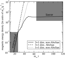
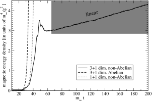
Fig. 2 shows an example from Ref. linear1 , showing the total energy density in soft magnetic fields as a function of time. This particular simulation was for moderate anisotropy and started from tiny initial conditions for the gauge fields. There is exponential growth at early times, due to the instability, and linear growth at late times. The linear growth does not represent continued growth of the unstable modes. Instead, the unstable modes stop growing but, through interactions, pump energy into a cascade of increasingly higher momentum, stable modes linear2 . This cascade takes the form of a gas of plasma excitations of the classical gauge field with momentum $q\gtrsim k_{\rm unstable}$, which are perturbative for $q\gg k_{\rm unstable}$. At late times, the total classical magnetic field energy density ${\cal E}^{B}_{\rm tot}={\textstyle{\frac{1}{2}}}B^{2}$ is dominated by the energy of these perturbative plasma excitations, rather than the energy density ${\cal E}^{B}_{*}\sim{\textstyle{\frac{1}{2}}}B_{*}^{2}$ of the softer ($k\sim k_{\rm unstable}$) unstable modes. For this reason, we cannot simply measure the total magnetic energy density ${\textstyle{\frac{1}{2}}}B^{2}$ at late times and take a square root to find the limiting size $B_{*}$ of the magnetic fields associated with unstable modes. And it is the soft fields $k\sim k_{\rm unstable}$, not the higher momentum plasmon excitations, which dominate the scattering of hard particles and so determine the evolution (17) relevant to bottom-up thermalization kminus2 : Even though the $k\sim k_{\rm unstable}$ modes carry less energy, they are more effective at scattering. To determine what we really want to know, we need some measurement other than the total magnetic energy density at a single late time.

Figure 2: Magnetic energy vs. time for a sample simulation from Ref. linear1 for moderate anisotropy, starting from a very small seed for the Weibel instability. The figures are the same except that the vertical axis is logarithmic in the left-hand figure and linear in the right-hand figure. The solid line is the result for non-abelian gauge theory in three spatial dimensions. For comparison, the dashed line shows a simulation in an abelian theory, and the dotted line shows a non-abelian simulation in one spatial dimension.

In this paper, we will use an indirect method to investigate anisotropy dependence which is relatively easy to implement. We will measure the slope $d{\cal E}^{B}_{\rm tot}/dt$ of the late-time linear growth of the total magnetic energy density and determine how it scales with anisotropy. Here is a model of how one might expect this slope to behave. The source of increasing total magnetic energy comes from the unstable modes, which take energy from the hard particles and, through interactions, dump it into the cascade of plasmons. As a thought experiment, imagine that half the energy density ${\cal E}^{B}_{*}$ in the unstable modes were abruptly transferred to the cascade of plasmons. How long would it take the unstable modes to grow back to their original, limiting size? Parametrically, the time should be of order the inverse instability growth rate $t\sim\gamma^{-1}\sim m_{\infty}^{-1}$. (Even though this is a perturbative estimate of the growth rate, it should still be parametrically correct in the region where perturbation theory starts to break down.) So the rate energy is pumped into the cascade can be expected to be of order $\gamma{\cal E}^{B}_{*}$:

$$\frac{d{\cal E}^{B}_{\rm tot}}{dt}\equiv\frac{d}{dt}\left({\textstyle{\frac{1}{2}}}B^{2}\right)_{\rm tot}\sim\gamma{\cal E}^{B}_{*}\sim\gamma B_{*}^{2}\sim\frac{m_{\infty}^{5}}{\theta^{2\nu}g^{2}},$$ (25)

where we have used the parametrization (17) of $B_{*}$. By measuring how this slope scales with $\theta$, we can extract the desired exponent $\nu$ that determines $B_{*}$, assuming that the physical argument for (25) is correct.

Following Ref. linear2 , we will generally start our simulations with large initial gauge fields so that we can quickly and easily get to the late-time limiting behavior. For extremely anisotropic hard particle distributions, this is a non-trivial choice: recent simulations BodekerRummukainen starting instead from tiny initial gauge fields find qualitatively different behavior. We will return to this point in Sec. II, where we argue that large initial conditions are appropriate to understanding how bottom-up thermalization is modified by instabilities.

We should note that the limiting field $B_{*}$ we have used to present a qualitative picture of the physics of instabilities is not a precisely defined quantity. Unlike the total magnetic field $B_{\rm tot}$, we know of no unique, convention-independent, gauge-invariant definition of the magnitude of $B_{*}$, and so $B_{*}$ is only useful for parametric estimates. In contrast, the observable (25) discussed above is gauge-invariant.

I.3 Overview of Results

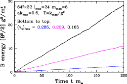
Figure 3: Examples of the linear growth of total magnetic energy with time. From bottom to top, the three curves have $k_{\rm max}/m_{\infty}=2.16$, $3.15$, and $4.10$ respectively (corresponding to the $N_{\Omega}=3$, 5, and 7 distributions described in Sec. III.1).

Fig. 3 shows an example of the total magnetic energy density ${\cal E}^{B}_{\rm tot}$ vs. time for three different anisotropies, starting from strong, non-perturbative initial conditions which we shall detail later. One way to parametrize the amount of anisotropy is to rewrite (12) as

$$\theta\sim\frac{m_{\infty}}{k_{\rm max}}\,,$$ (26)

where we compute $m_{\infty}/k_{\rm max}$ perturbatively for each background hard particle velocity distribution $\Omega({\bm{v}})$ [i.e. each distribution $f_{0}({\bm{p}})$] that we simulate. Fig. 3 shows increasing slope for increasing anisotropy. We will then rewrite the scaling form (25) in the form

$$\frac{g^{2}\,d{\cal E}^{B}_{\rm tot}/dt}{m_{\infty}^{4-2\nu}k_{\rm max}^{2\nu}\gamma_{*}}\sim\mbox{constant},$$ (27)

where we take $\gamma_{*}$ to be the largest unstable mode growth rate computed in perturbation theory. (This rate approaches $m_{\infty}/\sqrt{2}$ in the limit of extreme anisotropy ALM , but we have chosen to keep $\gamma_{*}$ explicit in our formula because the approach to this limit is a bit slow. Details will be given in Sec. III.1.)

Fig. 4 shows the left-hand side of (27) vs. our measure $m_{\infty}/k_{\rm max}$ of anisotropy for a variety of different simulations, plotted with exponents $\nu={\textstyle{\frac{1}{2}}}$, $1$, and $\tfrac{3}{2}$. Each point has systematic errors of order 15%. The $\nu=1$ version plausibly approaches a constant in the extreme anisotropy limit $m_{\infty}/k_{\rm max}\to 0$. The $\nu={\textstyle{\frac{1}{2}}}$ and $\nu=\tfrac{3}{2}$ figures clearly rule out $\nu\leq{\textstyle{\frac{1}{2}}}$ and $\nu\geq\tfrac{3}{2}$. Of the three possibilities $\nu=0$, $1$, and $2$ considered in (18), we conclude that only $\nu=1$ is consistent with this measurement.

Figure 4: The slope $d{\cal E}^{B}_{\rm tot}/dt$ of the linear growth of total magnetic field energy, measured in units of $m_{\infty}^{4-2\nu}k_{\rm max}^{2\nu}\gamma_{*}/g^{2}$, as a function of anisotropy for (a) $\nu={\textstyle{\frac{1}{2}}}$, (b) $\nu=1$, and (c) $\nu=\tfrac{3}{2}$. Simulation parameters are listed in Table 3 in Section III; squares are the default values and crosses are alternate values at the bottom of the table. The numbers by the data points indicate the order $N_{\Omega}$ of the distribution, as described in Sec. III.1.

II Large vs. small initial conditions

We have initialized our simulations with large initial gauge fields. In contrast, many simulations in the past, such as Fig. 2, have started from tiny initial gauge fields in order to observe the crossover from perturbative, exponential growth of instabilities to the limiting late-time behavior. Fig. 5 shows the difference for moderate anisotropy: we have superposed the tiny initial condition simulation of Fig. 2 (Ref. linear1 ) with an otherwise identical simulation starting from large intitial conditions. For tiny initial conditions, there is a significant spurt of continued exponential-like growth even after the field strength reaches non-perturbatively large values. It is only later, at much higher energy, that linear growth finally sets in. Bödeker and Rummukainen BodekerRummukainen have found that this spurt of post-non-perturbative exponential growth for tiny initial conditions becomes much more significant for extreme anisotropy. In their simulations for extreme anisotropy, they see only exponential-like growth at late times; they do not see late-time linear behavior at all. It is possible that the late-time behavior is ultimately linear but sets in at such large field energy that their simulations cannot reproduce it because of lattice spacing artifacts. But regardless, the full story of the development of plasma instabilities appears to be qualitatively different depending on whether or not one starts with large or tiny initial conditions.

Figure 5: The difference between tiny initial conditions, as in Fig. 2, and large initial conditions, similar to Ref. linear2 . (The large initial conditions were set as in Sec. III.3 but with $T=4m_{\infty}/3g^{2}$, $k_{\rm smear}=2m_{\infty}$, and squeeze $s=1.5$.)

Which type of initial condition is relevant to a new scenario of bottom-up thermalization? We argue that it is the case of non-perturbatively large initial conditions that we have investigated in this paper. Consider some time $\tau_{1}$ in the first stage of a new bottom-up scenario that accounts for instabilities, with $Q_{\rm s}\tau_{1}\gg 1$. We’ve already reviewed how the instability growth rate is large compared to the expansion rate $1/\tau_{1}$, and so the unstable modes will have grown to become non-perturbatively big (or perhaps larger). This population of unstable modes is depicted very crudely by the curve in the cartoon of Fig. 6. (In addition, higher momentum modes may be populated due to having been unstable at earlier times, or due to interactions.) It’s important to note that the unstable modes will grow to non-perturbative size regardless of how small the initial seed fields for those unstable modes are, because the instability growth rate is fast and quantum fluctuations will seed the unstable modes even if nothing else does.

Now consider what happens a little later, at time $\tau_{2}\equiv 2\tau_{1}$. The set of unstable modes shrinks a bit in $k$ space. Specifically, combining (12), (22), and (23), we have

$$k_{\rm max}\sim\frac{m_{\infty}}{\theta}\sim Q_{\rm s}\,(Q_{\rm s}\tau)^{-(1+2\nu)/[4(1+\nu)]}.$$ (28)

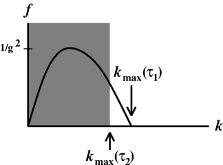
For definiteness, consider $\nu=1$, for which $k_{\rm max}\sim Q_{\rm s}\,(Q_{\rm s}\tau)^{-3/8}$. Then $k_{\rm max}$ decreases by a factor of $2^{-3/8}\simeq 0.77$ when time $\tau$ increases by a factor of 2, The unstable modes at the later time $\tau_{2}$ are therefore shown by the shaded area in Fig. 6, and we see that they are already initialized with non-perturbatively large fields because of the earlier instability growth at time $\tau_{1}$.

Figure 6: A cartoon of the occupation number $f(k)$ of unstable modes at time $\tau_{1}$, with the shaded area depicting those modes which are perturbatively unstable at the later time $\tau_{2}=2\tau_{1}$.

We have tried to make our argument general: Regardless of whether we start with large or small seeds for instability growth at $\tau=\tau_{1}$, we will then get large seeds for instability growth at later times such as $\tau_{2}=2\tau_{1}$. But the same argument means that we had large seeds at $\tau_{1}$ also because of yet earlier instability growth at time $\tau_{1}/2$. We can follow this argument all the way back to times of order the saturation time, when all the relevant modes of the fields started non-perturbatively large. We conclude that the typical unstable modes have high occupancies at all times during the initial stage of the new bottom-up scenario.

III Simulating extreme anisotropy

To simulate the non-abelian Vlasov equations (24), we need to discretize the arguments ${\bm{x}}$ and ${\bm{v}}$ of the fields $W({\bm{x}},{\bm{v}},t)$ and $A({\bm{x}},t)$. For ${\bm{x}}$, we put the system on a spatial lattice. For velocity ${\bm{v}}$, we follow Refs. BMR ; linear1 ; linear2 and expand in spherical harmonics $Y_{\ell m}({\bm{v}})$, truncating the expansion at some maximum value $\ell_{\rm max}$ of $\ell$:

$$W({\bm{x}},{\bm{v}},t)=\sum_{\ell=0}^{\ell_{\rm max}}\sum_{m}W_{\ell m}({\bm{x}},t)\,\hat{Y}_{\ell m}({\bm{v}}),$$ (29)

where our convention is to normalize the spherical harmonics so that the angular average of $\hat{Y}_{\ell m}({\bm{v}})\,\hat{Y}_{\ell^{\prime}m^{\prime}}({\bm{v}})$ is $\delta_{\ell\ell^{\prime}}\delta_{mm^{\prime}}$. (We place the hat over $\hat{Y}_{\ell m}$ as a reminder of this non-standard normalization convention.) The axi-symmetric, hard particle background velocity distribution $\Omega({\bm{v}})$ has the expansion

$$\Omega({\bm{v}})=\sum_{\ell=0}^{\ell_{\rm max}}\Omega_{\ell}\,\hat{Y}_{\ell 0}({\bm{v}})=\sum_{\ell=0}^{\ell_{\rm max}}\Omega_{\ell}(2\ell+1)^{1/2}\,P_{\ell}(v_{z}),$$ (30)

where the $P_{\ell}(x)$ are Legendre polynomials. The explicit form of the equations of motion (24) in terms of the $W_{\ell m}$’s is given in Ref. linear1 .

In practice, we must choose $\ell_{\rm max}$ large enough to obtain results close to the $\ell_{\rm max}\to\infty$ limit. More anisotropic distributions $\Omega({\bm{v}})$ will require larger $\ell_{\rm max}$ and therefore greater computational resources (both memory and time, to store and evolve more $W_{\ell m}$’s). Below, we first describe our choice of distributions $\Omega({\bm{v}})$ to simulate. Then we explain and justify our method for making simulations of very anisotropic distributions practical, which is to reduce the number of $W_{\ell m}$’s by limiting $m$ to $|m|\leq m_{\rm max}$ with $m_{\rm max}\simeq 6$.

III.1 Choice of hard particle distribution $f_{0}({\bm{p}})$

For a given maximum $\ell$, we would like to find a velocity distribution $\Omega({\bm{v}})$ of hard particles which is as anisotropic $(\theta\sim|v_{z}|\ll 1)$ as possible. To be physical, $\Omega({\bm{v}})$ should be non-negative. After some experimentation, we settled on the following form, parametrized by an integer order $N_{\Omega}$:

$$\Omega(v_{z})=\begin{cases}{\cal N}(1-v_{z}^{2})\phantom{{}^{2}}\prod_{i=1}^{n}(\alpha_{i}-v_{z}^{2})^{2},&\mbox{for $N_{\Omega}=2n+1$;}\\ {\cal N}(1-v_{z}^{2})^{2}\prod_{i=1}^{n}(\alpha_{i}-v_{z}^{2})^{2},&\mbox{for $N_{\Omega}=2n+2$;}\end{cases}$$ (31)

where the normalization ${\cal N}$ is chosen to satisfy our convention that the angular average $\Omega_{0}$ of $\Omega({\bm{v}})$ is one. We choose the $\alpha_{i}$ to minimize $\langle v_{z}^{2}\rangle$, performing the minimization numerically for each $N_{\Omega}$.

The expansion of $\Omega({\bm{v}})$ involves spherical harmonics with $l\leq L_{\Omega}\equiv 2N_{\Omega}$, and the corresponding coefficients $\Omega_{l}$ are listed in Appendix B for various choices of $N_{\Omega}$. We will see later, looking at the $\ell_{\rm max}$ dependence of results, that we can get close to the $\ell_{\rm max}\to\infty$ limit for a given $N_{\Omega}$ using $\ell_{\rm max}\gtrsim 1.5\,L_{\Omega}=3N_{\Omega}$.

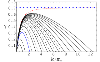
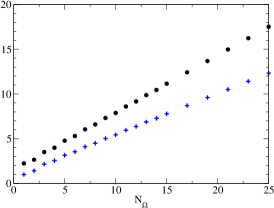
Table 2 summarizes basic properties of these distributions for various values of $N_{\Omega}$. Increasing anisotropy is signaled by decreasing $(v_{z})_{\rm rms}=\langle v_{z}^{2}\rangle^{1/2}$ and increasing $k_{\rm max}/m_{\infty}$. For graphical comparison, Fig. 7 shows, for different values of $N_{\Omega}$, the perturbative growth rates of unstable modes as a function of wavenumber $k$ in the case that ${\bm{k}}$ points exactly along the beam direction. For each distribution, $k_{\rm max}$ denotes the largest unstable momentum, $\gamma_{*}$ is the largest growth rate, and $k_{*}$ is the corresponding momentum. Figs. 8 and 9 show $k_{\rm max}$, $1/(v_{z})_{\rm rms}$, and $\gamma_{*}$ vs. $N_{\Omega}$. For comparison, the moderately anisotropic distribution previously simulated in Refs. linear1 ; linear2 is roughly comparable to our $N_{\Omega}=3$ distribution, and the most extremely anisotropic distribution simulated in Ref. BodekerRummukainen is roughly comparable to our $N_{\Omega}=15$ distribution.

$N_{\Omega}$	$(v_{z})_{\rm rms}$	$k_{\rm max}/m_{\infty}$	$k_{*}/m_{\infty}$	$\gamma_{*}/m_{\infty}$
1	0.4472	1	0.500	0.111
2	0.3780	1.414	0.649	0.191
3	0.2852	2.155	0.875	0.310
4	0.2506	2.542	0.979	0.354
5	0.2093	3.149	1.130	0.408
6	0.1887	3.542	1.221	0.435
7	0.1653	4.099	1.342	0.466
8	0.1516	4.500	1.424	0.484
9	0.1366	5.031	1.527	0.505
10	0.1269	5.438	1.602	0.518
11	0.1163	5.954	1.693	0.533
12	0.1091	6.365	1.763	0.543
13	0.1013	6.870	1.846	0.554
14	0.0957	7.285	1.911	0.562
15	0.0897	7.783	1.987	0.570
17	0.0805	8.693	2.119	0.583
19	0.0731	9.601	2.245	0.594
21	0.0668	10.508	2.361	0.603
23	0.0616	11.414	2.475	0.611
25	0.0571	12.319	2.583	0.618

Table 2: For each of the hard particle distributions designated by $N_{\Omega}$, the quantity $(v_{z})_{\rm rms}=\langle v_{z}^{2}\rangle^{1/2}$ measures the narrowness of the velocity distribution about the transverse plane. $k_{\rm max}$ is the maximum unstable wavenumber. $\gamma_{*}$ is the largest perturbative growth rate of the field modes ${\bm{A}}({\bm{k}})$ and corresponds to wavenumber $k_{*}$. The corresponding perturbative growth rate of magnetic energy is $2\gamma_{*}$.

Figure 7: Perturbative instability growth rates $\gamma(k)$ vs. $k/m_{\infty}$ for the values of $N_{\Omega}$ listed in Table 2. Solid (dashed) black lines are odd (even) $N_{\Omega}$, staring with $N_{\Omega}=1$ at the bottom and running up to $N_{\Omega}=25$ at the top. The horizontal dotted line is the maximum possible $\gamma$, which is $1/\sqrt{2}$, and the dashed line approaching it is the case $N_{\Omega}=\infty$, given in Ref. ALM .

Figure 8: The values of $1/(v_{z})_{\rm rms}$ (circles) and $k_{\rm max}/m_{\infty}$ (crosses) plotted vs. $N_{\Omega}$.

Figure 9: The maximum growth rate $\gamma_{*}$ (in units of $m_{\infty}$) plotted vs. $N_{\Omega}$. The top of the graph represents the $N_{\Omega}\to\infty$ limit of $\gamma_{*}\to m_{\infty}/\sqrt{2}$ ALM .

III.2 A reduced set of $Y_{\ell m}$’s

The expansion of extremely anisotropic distributions $\Omega(v_{z})$ in spherical harmonics $Y_{\ell m}({\bm{v}})$ requires large $\ell$ values but, due to the axial symmetry of the distribution, only the $m$ value $m=0$. The dynamics (24b) of the fluctuations $W({\bm{v}},{\bm{x}},t)$ in the distribution, however, will create $W_{lm}$’s with non-zero values of $m$. We might hope that only small $m$ values turn out to be significant. Though there will be a lot of rapid variation in how $W({\bm{v}},{\bm{x}},t)$ depends on $v_{z}$, because we are studying the case of extreme anisotropy, there might be relatively smooth dependence on $(v_{x},v_{y})$. We will verify this picture below using simulation data, and also give some qualitative arguments why one might expect it. We can take advantage of this smooth dependence by placing an upper bound $|m|\leq m_{\rm max}$ on the range of $m$ we include in our simulations, so that the expansion (29) of $W$ becomes

$$W({\bm{x}},{\bm{v}},t)=\sum_{\ell=0}^{\ell_{\rm max}}\sum_{\begin{subarray}{c}|m|\leq\ell\\ |m|\leq m_{\rm max}\end{subarray}}W_{\ell m}({\bm{x}},t)\,\hat{Y}_{\ell m}({\bm{v}}),$$ (32)

For unrestricted $m$’s, the total number of $W_{\ell m}$ at each lattice site (and so the resources required for the simulations) would grow quadratically with $\ell_{\rm max}$. For a fixed bound $|m|\leq m_{\rm max}$, however, they only grow linearly for large $\ell_{\rm max}$, making simulations of extreme anisotropy practical.

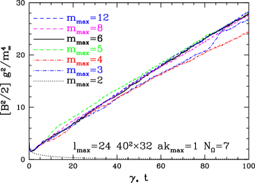
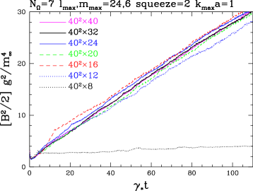
Fig. 10 shows an example of linear growth of total magnetic field energy for $N_{\Omega}=7$ simulations with $\ell_{\rm max}=24$ and several different values of $m_{\rm max}$. As can be seen, $m_{\rm max}=6$ is large enough to reproduce the correct ($m_{\rm max}\to\infty$) slope, and this is the value of $m_{\rm max}$ we will use in our simulations.

Figure 10: Linear growth of the total magnetic energy with time for several different values of $m_{\rm max}$. The parameters are the same as our canonical $N_{\Omega}=7$ simulation except the box size is $40^{2}\times 32$ and the squeeze factor is only 2.

In previous work on simulations for moderate anisotropy linear2 , we found that the systematic errors arising from a finite cut off $\ell_{\rm max}$ on $\ell$ could be reduced by damping the dynamics of modes with $\ell$ near the cut-off. We have slightly improved this method and extended it to apply also to the new cut-off $m_{\rm max}$ on $m$. Details are given in Appendix C. Such damping has been used in all the simulations reported in this paper.

The real test of the viability of using relatively small $m_{\rm max}$ cut-offs comes from simulations, such as Fig. 10. However, one can get some rough idea of why it can work by considering perturbative formulas for some of the important features of unstable modes and the resulting cascade of plasmons. If we treat the gauge field perturbatively in the $W$ equation (24b), replacing $D_{\mu}$ by $\partial_{\mu}$, we can Fourier transform from $({\bm{x}},t)$ to $({\bm{k}},\omega)$ and then solve for $W$:

$$W({\bm{v}},{\bm{k}},\omega)=im_{\infty}^{2}\;(\omega-{\bm{v}}\cdot{\bm{k}})^{-1}\left[{\bm{E}}({\bm{k}},\omega)\cdot(2{\bm{v}}-{\bm{\nabla}}_{\bm{v}})+{\bm{B}}({\bm{k}},\omega)\cdot({\bm{v}}\times{\bm{\nabla}}_{\bm{v}})\right]\Omega(v_{z})\,.$$ (33)

Together, the factors to the right of the $(\omega-{\bm{v}}\cdot{\bm{k}})^{-1}$ in this formula only generate ${\bm{v}}_{\perp}$ dependence with $|m|\leq 1$. All higher $m$ components in the result for $W$ are generated by the factor

$$(\omega-{\bm{v}}\cdot{\bm{k}})^{-1}=(\omega-{\bm{v}}_{\perp}\cdot{\bm{k}}_{\perp}-v_{z}k_{z})^{-1}.$$ (34)

Now consider the dominant unstable mode. As mentioned earlier, this mode has ${\bm{k}}$ along the $z$ axis (for the type of anisotropy we consider), and so ${\bm{k}}_{\perp}=0$. Then the factor (34) has no ${\bm{v}}_{\perp}$ dependence, and so the $W$ field which describes the dominant instability involves only $|m|\leq 1$.

As another example, consider the dispersion relation of transverse plasmons. A standard method for deriving the dispersion relation is to insert the result for $W$ into the Yang-Mills equation (24a), which generates the hard-loop self-energy correction to the vacuum relation $\omega^{2}=k^{2}$. How much will we disturb this dispersion relation if we throw away modes of $W$ with $m>m_{\rm max}$? For high momentum plasmons ($k\gg m_{\infty}$), such as those that dominate the cascade at late times, the effect is tiny simply because all medium effects to the dispersion relation are tiny in this limit. For very low momentum plasmons ($k\ll\omega\sim m_{\infty}$), we can ignore the ${\bm{v}}\cdot{\bm{k}}$ altogether in (34), and then the $W$ field will again have only $|m|\leq 1$ components. It is only for intermediate momentum plasmons ($k\sim m_{\infty}$) that finite $m_{\rm max}$ does violence to the plasmon dispersion relation. However, (34) is a fairly smooth function of ${\bm{v}}_{\perp}$ in this regime because the denominator never gets close to zero for $k\sim m_{\infty}$ plasmons ($\omega$ and $\omega-k$ are both of order $m_{\infty}$), and so (34) and therefore $W$ can be reasonably approximated by a superposition of relatively low $m$’s.

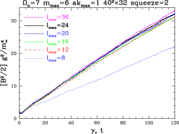
Finally, we should check that we have chosen large enough values of $\ell_{\rm max}$ in our simulations. In general, we find that $\ell_{\rm max}\sim 3N_{\Omega}$ is quite adequate. As an example, Fig. 11 shows the $\ell_{\rm max}$ dependence of $N_{\Omega}=7$ simulations for fixed $m_{\rm max}=6$. Our standard simulation choice for $\ell_{\rm max}$ is 24 for $N_{\Omega}=7$. See Table 3 for our default simulation parameters in other cases.

Figure 11: Linear growth of the total magnetic energy with time for several different values of $\ell_{\rm max}$, and fixed $m_{\rm max}=6$, for the hard particle distribution $N_{\Omega}=7$.

$N_{\Omega}$	$ak_{\rm max}$	$\ell_{\rm max}$	squeeze $s$	volume
3	0.6	24	1.5	$64^{2}\times 32$
4	0.6	24	2	$64^{2}\times 32$
5	0.8	24	2.5	$64^{2}\times 32$
6	0.8	24	3	$64^{2}\times 32$
7	1.0	24	3.5	$64^{2}\times 32$
8	1.0	32	3.5	$64^{2}\times 32$
9	1.0	32	3.5	$64^{2}\times 32$
11	1.0	40	3.5	$64^{2}\times 32$
13	1.0	48	3.5	$64^{2}\times 32$
15	1.0	56	3.5	$64^{2}\times 32$
25	1.2	80	3	$64^{2}\times 28$
5	0.6	24	2.5	$64^{2}\times 32$
6	0.6	24	3.0	$64^{2}\times 32$
7	0.6	24	3.5	$64^{2}\times 32$
7	0.8	24	3.0	$64^{2}\times 32$

Table 3: The default parameters for our simulations and their initialization, as a function of $N_{\Omega}$. The corresponding values of $k_{\rm max}$ are given in Table 2. Other default parameters include $m_{\rm max}=6$, initial temperature $T=k_{\rm max}/g^{2}$, and initial smearing wavenumber $k_{\rm smear}=k_{\rm max}$. The simulations below the horizontal line correspond to the crosses in Fig. 4.

III.3 Initial conditions

Following Ref. linear2 , we use strong, non-perturbative initial conditions for the magnetic field ${\bm{B}}$, so that the system starts linear energy growth behavior as quickly as possible. The electric and $W$ fields are, for simplicity, initialized to zero. In order to see the linear energy growth associated with cascade development as early as possible, it is advantageous to choose initial conditions which do not significantly populate modes with large wavenumber.

In the moderate anisotropy simulations of Ref. linear2 , the initial magnetic field was constructed by taking a thermal initial state with temperature $T=2m_{\infty}/g^{2}$ and then performing gauge-invariant smearing (sometimes called cooling) of the configuration to eliminate wavenumbers $k\gg m_{\infty}$. In perturbative language, this cooling corresponds to replacing the initial thermal field ${\bm{A}}_{\rm therm}$ by

$${\bm{A}}({\bm{k}})={\bm{A}}_{\rm therm}({\bm{k}})\exp(-k^{2}/k_{\rm smear}^{2}),$$ (35)

where $\tau=1/k_{\rm smear}^{2}$ is the smearing parameter. In Ref. linear2 , we chose $k_{\rm smear}=2m_{\infty}$.

Here, we follow a similar procedure, but the unstable modes that we want to initially populate are generally more extremely anisotropic, having $(k_{\perp},k_{z})\sim(m_{\infty},k_{\rm max})$ with $k_{\rm max}\gg m_{\infty}$. We have found that it helps to arrange a related anisotropy of our initial fields by squeezing the initial distribution in the $z$ direction. In perturbative language, our initial choice corresponds to

$$({\bm{A}}_{\perp},A_{z})[{\bm{k}}]=({\bm{A}}_{\perp,{\rm therm}}/s,A_{z,{\rm therm}})[s{\bm{k}}_{\perp},k_{z}]\exp\Big{(}-(s^{2}k_{\perp}^{2}+k_{z}^{2})/k_{\rm smear}^{2}\Big{)},$$ (36)

where $s$ is the squeezing factor. In our simulations, we have generally chosen $T=k_{\rm max}/g^{2}$, $k_{\rm smear}=k_{\rm max}$, and $s$ between $1.5$ and $3.5$ depending on the amount of anisotropy. See Table 3 for our default simulation parameters.

III.4 Lattice spacing and volume

It is important to check that the lattice volume is large enough to be in the infinite volume limit and the spacing is small enough to be in the continuum limit; otherwise the lattice calculation is not simulating the desired continuum physics. It would be prohibitive to check this at every lattice spacing, so we have “spot checked” this at a few levels of anisotropy, with the most thorough study at $N_{\Omega}=7$ and $N_{\Omega}=15$.

For highly anisotropic lattices, the physical scales possibly relevant to out problem parametrically span a range from $m_{\infty}$ to $k_{\rm max}$. One might worry that, as particle distributions are taken more and more anisotropic, it becomes harder and harder to span these scales with a computationally practical lattice. Naively, to be perfectly safe, we would like physical lattice dimensions $L\gg 2\pi/m_{\infty}$ and lattice spacings $a\ll 2\pi/k_{\rm max}$. In this section, we’ll see how well we do with lattices of practical size.

III.4.1 Physical volume

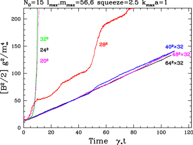
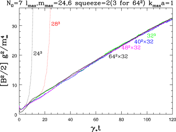
Figs. 12 and 13 show the volume dependence, at fixed lattice spacing, of the evolution of magnetic energy with time. The first figure is for the $N_{\Omega}{=}7$ hard particle distribution. The second figure is for $N_{\Omega}{=}15$, the second most anisotropic distribution included in our results of Fig. 4. Our default lattice size of $64^{2}\times 32$ corresponds to approximately $(15.6/m_{\infty})^{2}\times(7.8/m_{\infty})$ for $N_{\Omega}=7$ and $(8.2/m_{\infty})^{2}\times(4.1/m_{\infty})$ for $N_{\Omega}=15$. For small volumes, the simulations produced exponential rather than linear growth. But linear growth appears at large enough volume, and a comparison of the large volume curves suggests that our default lattice size of $64^{2}\times 32$ is adequate, even for our highly anisotropic distributions.

Figure 12: Linear growth of the total magnetic energy with time for several different physical volumes, at fixed lattice spacing, for the hard particle distribution $N_{\Omega}=7$.

Figure 13: As Fig. 12 but for the more anisotropic distribution $N_{\Omega}=15$.

In order to be able to run our simulations on desktop computers, we by default took the physical lattice size $L_{z}$ in the $z$ direction to be half that in the $x$ and $y$ directions. This choice is motivated by the fact that, in the highly anisotropic case, unstable modes have parametrically smaller wavelength in the $z$ direction ($\sim 1/k_{\rm max}$) than in the perpendicular directions ($\sim 1/m_{\infty}$). Of course, that doesn’t exclude the possibility that stable modes with size $k_{x}\sim k_{y}\sim k_{z}\sim 1/m_{\infty}$ might be important in the development of linear growth, and so we should investigate the matter with simulations. Fig. 14 isolates the effect of varying $L_{z}$ while holding the $L_{x}$ and $L_{y}$ fixed. (Note that $L_{x}=L_{y}$ is smaller here than in Fig. 12.) An $L_{z}$ that is half of $L_{x}=L_{y}$ appears adequate for reproducing the large-$L_{z}$ linear slope.

Figure 14: Linear growth of the total magnetic energy with time on an $L_{\perp}^{2}\times L_{z}$ lattice for several different choices of $L_{z}$ (at fixed lattice spacing), for the hard particle distribution $N_{\Omega}=7$.

III.4.2 Lattice spacing

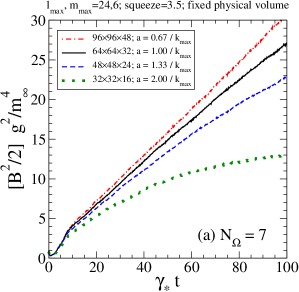
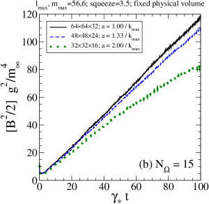
Fig. 15 shows how our simulations depend on lattice spacing for fixed physical volume, for the distributions $N_{\Omega}=7$ and $N_{\Omega}=15$. In order to isolate the effect of lattice spacing, we have used the same initial conditions for all these simulations. More precisely, we generated initial conditions for the finest lattice ($96{\times}96{\times}48$), and then we used blocking to generate similar initial conditions for the coarser lattices.

Figure 15: Linear growth of the total magnetic energy with time for several different lattice spacings, at fixed physical volume $L_{x}{\times}L_{y}{\times}L_{z}=(64/k_{\rm max}){\times}(64/k_{\rm max}){\times}(32/k_{\rm max})$, for the hard particle distributions (a) $N_{\Omega}=7$ and (b) $N_{\Omega}=15$.

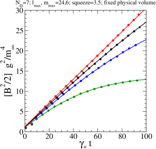
At all but the finest lattice spacing in Fig. 15a, one can see some curvature to the late-time “linear” growth behavior. This curvature is a lattice artifact, but it means that we need a procedure for extracting a single “slope” from such simulations, in order to present results such as Fig. 4. Note that the coarsest lattice spacing results in Fig. 15 look like sections of tanh curves, after an initial transient. Inspired by this observation, we have chosen to fit each of our energy curves to the form

$${\textstyle{\frac{1}{2}}}B^{2}(t)=\sigma\,t_{1}\tanh\left(\frac{t-t_{0}}{t_{1}}\right)$$ (37)

for $\gamma_{*}t>10$. The parameters of the fit are $s$, $t_{0}$, and $t_{1}$. We take the slope $\sigma$ (the slope of the tanh at zero argument) to be our result for $d{\cal E}^{B}_{\rm tot}/dt$. The curving of the tanh is controlled by $t_{1}$, and $t_{1}$ should go to infinity as we approach the continuum limit.

Figure 16: The curves of Fig. 15a, all shown here as dotted lines, superposed with solid lines corresponding to the fits of Eq. (37).

Fig. 16 shows the tanh fits for the simulations of Fig. 15a: the fits work extremely well. The solid circles in Fig. 17 show how the fit of the slope $\sigma$ depends on the lattice spacing. The $x$ axis is chosen to be the square of the lattice spacing because the discretization errors in our lattice implementation first arise at this order. Extrapolating by eye to the continuum limit, we estimate that our default lattice spacing of $ak_{\rm max}=1$ for these distributions has lattice spacing errors no larger than roughly 10%. In contrast, the open circles in Figs. 17 show the behavior of $1/t_{1}$, which is a lattice artifact and approaches zero in the continuum limit (corresponding to purely linear growth).

Figure 17: Fit parameters for the (a) $N_{\Omega}=7$ and (b) $N_{\Omega}=15$ simulations of Fig. 15 as a function of lattice spacing squared. Solid circles are the slope $\sigma$ (and so $d{\cal E}^{B}_{\rm tot}/dt$) in units of $m_{\infty}^{4}\gamma_{*}/g^{2}$, and open circles are $1/t_{1}$ in units of $(100/\gamma_{*})^{-1}$.

IV Conclusion

The goal of this paper has been to understand how, in the weak coupling limit, the late-time behavior of Weibel instabilities scales with hard particle anisotropy. We can use the smallness of $\theta\equiv v_{z}$, characterizing the angular distribution of hard particles, as a measure of anisotropy. Through simulations, we have examined the slope $d{\cal E}_{\rm tot}^{B}/dt$ of the late-time linear growth in the total magnetic energy of soft gauge fields and found that the scaling of this slope is consistent with $\theta^{-2}$ and not consistent with $\theta^{-1}$ or $\theta^{-3}$. If we accept the simple model outlined in section I.2 of the physics behind $d{\cal E}_{\rm tot}^{B}/dt$, this result implies that the limiting magnetic field strength $B_{*}$ of Weibel unstable modes scales with anisotropy as $\theta^{-1}$ and is of order

$$B_{*}\sim\frac{m_{\infty}^{4}}{\theta g}\,.$$ (38)

Of course, it would be better not to rely on such indirect arguments. A goal for future work should be to check the consistency of this conclusion with alternative measurements.

Appendix A The Nielsen-Olesen limit

At one time, it was conjectured that exponential instability growth would continue beyond the point where non-abelian interactions became important because the fields would dynamically align themselves into a commuting set of color directions AL . The fields would then be effectively abelian and could continue growing, just like the purely abelian case shown by the dashed line in Fig. 2. This conjecture seemed borne out by early simulations in one spatial dimension RRS , such as shown by the dotted line in that figure. At the time, Berndt Müller berndt predicted that three-dimensional instability growth would eventually have to stop because, even if the gauge fields did abelianize, Nielsen-Olesen instabilities NielsenOlesen would eventually destroy nearly-abelian configurations as the fields continue to grow.

In this appendix, we will discuss the largest field strength allowed for nearly-abelian Weibel unstable modes before Nielsen-Olesen instabilities appear. A brief review of Nielsen-Olesen instabilities in the context of Weibel instabilities for moderate anisotropy can be found in Ref. ArnoldLeang . Here, we generalize to the case of extreme anisotropy.

First imagine a situation where there was a large, constant, homogeneous magnetic field $B_{0}$ that lies within an abelian subgroup of the non-abelian gauge group. In our application, this could represent a large magnetic field that was created by the Weibel instability and that might have abelianized due to non-linear dynamics, and that we are looking at this field on small enough time and distance scales that we can treat it as constant. For the sake of definiteness, consider SU(2) gauge theory and a background magnetic field

$$B_{i}^{a}({\bm{x}},t)={\bm{B}}_{0}\,\delta^{a3},$$ (39)

where $a$ is the adjoint color index. Now one can investigate the dispersion relation of fluctuations about this background field, including fluctuations involving other, non-commuting color directions. Ignoring hard particle effects, the result is NielsenOlesen

$$\omega^{2}=q_{\parallel}^{2}+(n+{\textstyle{\frac{1}{2}}})2|Q|gB_{0}-2m_{\rm s}QgB_{0},$$ (40)

where $q_{\parallel}$ is the component of momentum parallel to ${\bm{B}}_{0}$; $n$ is the Landau orbit quantum number for circular motion in the plane transverse to ${\bm{B}}_{0}$; $m_{\rm s}=0$ or $\pm 1$ is the component, in the direction of ${\bm{B}}_{0}$, of the spin of a gauge excitation; and $Q=0$ or $\pm 1$ is the charge of that excitation under the color generator $T^{3}$. The last term in (40) represents the interaction energy of a gauge particle’s magnetic moment with the magnetic field. If we look at the lowest Landau orbits ($n=0$) and the sector $Q=m_{\rm s}=\pm 1$, we get

$$\omega^{2}=q_{\parallel}^{2}-gB_{0}.$$ (41)

$\omega^{2}$ is then negative for $q_{\parallel}\leq\sqrt{gB_{0}}$. This is the Nielsen-Olesen instability.

In our application, the magnetic fields are not homogeneous. In order to make that approximation, the radius associated with the lowest Landau orbit should be small enough to fit in a region of roughly constant magnetic field. This radius is $R\sim 1/\sqrt{gB_{0}}$. The dominant Weibel-unstable modes have $B$ roughly orthogonal to the $z$ axis, and wavenumber of order $(k_{\perp},k_{z})\sim(m_{\infty},k_{\rm max})$. So, to produce the Nielsen-Olesen instability, we need both $R\ll 1/k_{\perp}$ and $R\ll 1/k_{z}$. In the case of extreme anisotropy, the latter is the stricter constraint, equivalent to

$$\frac{1}{\sqrt{gB_{0}}}\ll\frac{1}{k_{\rm max}}\sim\frac{\theta}{m_{\infty}}\,,$$ (42)

which requires

$$B_{0}\gg\frac{m_{\infty}^{2}}{\theta^{2}g}\,.$$ (43)

As the magnetic field grows, Nielsen-Olesen instabilities will then first appear for

$$B_{0}\sim\frac{m_{\infty}^{2}}{\theta^{2}g}\,.$$ (44)

This corresponds to the case $\nu=2$ in (17).

There are a few approximations left to check. First, the Nielsen-Olesen analysis assumed that $B_{0}$ was constant in time. The typical Nielsen-Olesen instability growth times generated by (41) will be of order $(-\omega^{2})^{-1/2}\sim 1/\sqrt{gB}$. This will be small compared to the (abelianized) Weibel instability growth time $\gamma_{*}^{-1}\sim m_{\infty}^{-1}$ when (43) is satisfied. Secondly, we have ignored hard particle effects throughout. In general, the magnitude of the soft self-energy $\Pi$ due to hard particles can be as large as order $k_{\rm max}^{2}\sim m_{\infty}^{2}/\theta^{2}$, depending on direction and $\omega/k$. But this is small enough that $\Pi$ will be a small correction to $gB_{0}$ in the dispersion relation (41) when (43) is satisfied.

The results of this paper suggest that $\nu=1$ rather than $\nu=2$. It may well be that Nielsen-Olesen effects limit the Weibel instability growth of nearly abelian fields. The results of this paper simply suggest that, if one starts with large amplitude, nonperturbative, non-abelian initial conditions, then generic non-perturbative interactions are sufficient to stop growth earlier, at lower field strength than (44).

Appendix B The coefficients $\Omega_{\ell}$

In principle, anyone who wanted to know the specific values of $\Omega_{l}$ for our distributions could reproduce them from the procedure outlined in the text. However, we found that avoiding numerical round-off errors in determining $\Omega_{l}$ for large $N_{\Omega}$ required some care. So we will explicitly give our distributions here.

$N_{\Omega}=1$: $\Omega_{0}=1$, $\Omega_{2}=-1/\sqrt{5}$

$N_{\Omega}=2$: $\Omega_{0}=1$, $\Omega_{2}=-2\sqrt{5}/7$, $\Omega_{4}=1/7$

$N_{\Omega}=3$: $\alpha_{1}=0.585310$; $\Omega_{0}=1$, $\Omega_{2}=-0.845154$, $\Omega_{4}=0.474960$, $\Omega_{6}=-0.148398$

$N_{\Omega}=4$: $\alpha_{1}=0.482673$; $\Omega_{0}=1$, $\Omega_{2}=-0.907458$, $\Omega_{4}=0.589250$, $\Omega_{6}=-0.277350$, $\Omega_{8}=0.063395$

$N_{\Omega}=5$: $\alpha_{1}=0.350109$, $\alpha_{2}=0.759931$; $\Omega_{0}=1$, $\Omega_{2}=-0.971104$, $\Omega_{4}=0.730670$, $\Omega_{6}=-0.449643$, $\Omega_{8}=0.216519$, $\Omega_{10}=-0.063736$

$N_{\Omega}=6$: $\alpha_{1}=0.292253$, $\alpha_{2}=0.672147$; $\Omega_{0}=1$, $\Omega_{2}=-0.998631$, $\Omega_{4}=0.794155$, $\Omega_{6}=-0.544163$, $\Omega_{8}=0.311154$, $\Omega_{10}=-0.138336$, $\Omega_{12}=0.032712$

$N_{\Omega}=7$: $\alpha_{1}=0.228412$, $\alpha_{2}=0.545787$, $\alpha_{3}=0.845543$; $\Omega_{0}=1$, $\Omega_{2}=-1.026410$, $\Omega_{4}=0.864186$, $\Omega_{6}=-0.650680$, $\Omega_{8}=0.436901$, $\Omega_{10}=-0.249727$, $\Omega_{12}=0.113554$, $\Omega_{14}=-0.032709$

$N_{\Omega}=8$: $\alpha_{1}=0.194863$, $\alpha_{2}=0.478948$, $\alpha_{3}=0.776881$; $\Omega_{0}=1$, $\Omega_{2}=-1.040916$, $\Omega_{4}=0.901356$, $\Omega_{6}=-0.712570$, $\Omega_{8}=0.512936$, $\Omega_{10}=-0.329365$, $\Omega_{12}=0.179614$, $\Omega_{14}=-0.077926$, $\Omega_{16}=0.018926$

$N_{\Omega}=9$: $\alpha_{1}=0.159625$, $\alpha_{2}=0.400532$, $\alpha_{3}=0.671219$, $\alpha_{4}=0.892835$; $\Omega_{0}=1$, $\Omega_{2}=-1.055491$, $\Omega_{4}=0.940673$, $\Omega_{6}=-0.778554$, $\Omega_{8}=0.600618$, $\Omega_{10}=-0.424975$, $\Omega_{12}=0.271564$, $\Omega_{14}=-0.149879$, $\Omega_{16}=0.066253$, $\Omega_{18}=-0.018902$,

$N_{\Omega}=10$: $\alpha_{1}=0.138840$, $\alpha_{2}=0.353981$, $\alpha_{3}=0.608348$, $\alpha_{4}=0.839259$; $\Omega_{0}=1$, $\Omega_{2}=-1.064055$, $\Omega_{4}=0.963974$, $\Omega_{6}=-0.819732$, $\Omega_{8}=0.656358$, $\Omega_{10}=-0.490737$, $\Omega_{12}=0.337910$, $\Omega_{14}=-0.210147$, $\Omega_{16}=0.111992$, $\Omega_{18}=-0.047971$, $\Omega_{20}=0.011893$

$N_{\Omega}=11$: $\alpha_{1}=0.117460$, $\alpha_{2}=0.303204$, $\alpha_{3}=0.531249$, $\alpha_{4}=0.753079$, $\alpha_{5}=0.921475$; $\Omega_{0}=1$, $\Omega_{2}=-1.072643$, $\Omega_{4}=0.988135$, $\Omega_{6}=-0.862564$, $\Omega_{8}=0.717049$, $\Omega_{10}=-0.563740$, $\Omega_{12}=0.417060$, $\Omega_{14}=-0.285605$, $\Omega_{16}=0.177636$, $\Omega_{18}=-0.096139$, $\Omega_{20}=0.041819$, $\Omega_{22}=-0.011875$

$N_{\Omega}=12$: $\alpha_{1}=0.103801$, $\alpha_{2}=0.270617$, $\alpha_{3}=0.481526$, $\alpha_{4}=0.697580$, $\alpha_{5}=0.879018$; $\Omega_{0}=1$, $\Omega_{2}=-1.078115$, $\Omega_{4}=1.003612$, $\Omega_{6}=-0.890930$, $\Omega_{8}=0.757648$, $\Omega_{10}=-0.614860$, $\Omega_{12}=0.473819$, $\Omega_{14}=-0.343760$, $\Omega_{16}=0.230949$, $\Omega_{18}=-0.141010$, $\Omega_{20}=0.074196$, $\Omega_{22}=-0.031545$, $\Omega_{24}=0.007947$

$N_{\Omega}=13$: $\alpha_{1}=0.089898$, $\alpha_{2}=0.236254$, $\alpha_{3}=0.425611$, $\alpha_{4}=0.627277$, $\alpha_{5}=0.808562$, $\alpha_{6}=0.940062$; $\Omega_{0}=1$, $\Omega_{2}=-1.083597$, $\Omega_{4}=1.019484$, $\Omega_{6}=-0.920055$, $\Omega_{8}=0.800595$, $\Omega_{10}=-0.669524$, $\Omega_{12}=0.537151$, $\Omega_{14}=-0.410252$, $\Omega_{16}=0.296157$, $\Omega_{18}=-0.198861$, $\Omega_{20}=0.121655$, $\Omega_{22}=-0.065052$, $\Omega_{24}=0.028013$, $\Omega_{26}=-0.007936$

$N_{\Omega}=14$: $\alpha_{1}=0.080480$, $\alpha_{2}=0.212901$, $\alpha_{3}=0.387457$, $\alpha_{4}=0.579149$, $\alpha_{5}=0.760545$, $\alpha_{6}=0.905790$; $\Omega_{0}=1$, $\Omega_{2}=-1.087305$, $\Omega_{4}=1.030254$, $\Omega_{6}=-0.940283$, $\Omega_{8}=0.830602$, $\Omega_{10}=-0.708871$, $\Omega_{12}=0.583371$, $\Omega_{14}=-0.460883$, $\Omega_{16}=0.347161$, $\Omega_{18}=-0.247263$, $\Omega_{20}=0.163617$, $\Omega_{22}=-0.098747$, $\Omega_{24}=0.051563$, $\Omega_{26}=-0.021818$, $\Omega_{28}=0.005568$

$N_{\Omega}=15$: $\alpha_{1}=0.070949$, $\alpha_{2}=0.188716$, $\alpha_{3}=0.346338$, $\alpha_{4}=0.523712$, $\alpha_{5}=0.698217$, $\alpha_{6}=0.847595$, $\alpha_{7}=0.952782$; $\Omega_{0}=1$, $\Omega_{2}=-1.091017$, $\Omega_{4}=1.041226$, $\Omega_{6}=-0.960895$, $\Omega_{8}=0.861825$, $\Omega_{10}=-0.750085$, $\Omega_{12}=0.633157$, $\Omega_{14}=-0.516209$, $\Omega_{16}=0.405183$, $\Omega_{18}=-0.303840$, $\Omega_{20}=0.215905$, $\Omega_{22}=-0.143127$, $\Omega_{24}=0.086609$, $\Omega_{26}=-0.045945$, $\Omega_{28}=0.019653$, $\Omega_{30}=-0.005561$

$N_{\Omega}=17$: $\alpha_{1}=0.057385$, $\alpha_{2}=0.153941$, $\alpha_{3}=0.286217$, $\alpha_{4}=0.440599$, $\alpha_{5}=0.601196$, $\alpha_{6}=0.751477$, $\alpha_{7}=0.875973$, $\alpha_{8}=0.961858$; $\Omega_{0}=1$, $\Omega_{2}=-1.096274$, $\Omega_{4}=1.056905$, $\Omega_{6}=-0.990855$, $\Omega_{8}=0.907738$, $\Omega_{10}=-0.812101$, $\Omega_{12}=0.709497$, $\Omega_{14}=-0.603863$, $\Omega_{16}=0.499893$, $\Omega_{18}=-0.400800$, $\Omega_{20}=0.310023$, $\Omega_{22}=-0.229608$, $\Omega_{24}=0.161402$, $\Omega_{26}=-0.106052$, $\Omega_{28}=0.063689$, $\Omega_{30}=-0.033601$, $\Omega_{32}=0.014305$, $\Omega_{34}=-0.004046$

$N_{\Omega}=19$: $\alpha_{1}=0.047353$, $\alpha_{2}=0.127821$, $\alpha_{3}=0.239919$, $\alpha_{4}=0.374139$, $\alpha_{5}=0.519102$, $\alpha_{6}=0.662513$, $\alpha_{7}=0.792211$, $\alpha_{8}=0.897196$, $\alpha_{9}=0.968556$; $\Omega_{0}=1$, $\Omega_{2}=-1.100133$, $\Omega_{4}=1.068574$, $\Omega_{6}=-1.013442$, $\Omega_{8}=0.942914$, $\Omega_{10}=-0.860525$, $\Omega_{12}=0.770493$, $\Omega_{14}=-0.675846$, $\Omega_{16}=0.580283$, $\Omega_{18}=-0.486451$, $\Omega_{20}=0.397320$, $\Omega_{22}=-0.314853$, $\Omega_{24}=0.241036$, $\Omega_{26}=-0.176940$, $\Omega_{28}=0.123418$, $\Omega_{30}=-0.080579$, $\Omega_{32}=0.048126$, $\Omega_{34}=-0.025290$, $\Omega_{36}=0.010730$, $\Omega_{38}=-0.003034$

$N_{\Omega}=21$: $\alpha_{1}=0.039729$, $\alpha_{2}=0.107746$, $\alpha_{3}=0.203686$, $\alpha_{4}=0.320731$, $\alpha_{5}=0.450563$, $\alpha_{6}=0.583957$, $\alpha_{7}=0.711432$, $\alpha_{8}=0.823930$, $\alpha_{9}=0.913455$, $\alpha_{10}=0.973637$; $\Omega_{0}=1$, $\Omega_{2}=-1.103050$, $\Omega_{4}=1.077489$, $\Omega_{6}=-1.030870$, $\Omega_{8}=0.970394$, $\Omega_{10}=-0.898899$, $\Omega_{12}=0.819660$, $\Omega_{14}=-0.735041$, $\Omega_{16}=0.647973$, $\Omega_{18}=-0.560615$, $\Omega_{20}=0.475461$, $\Omega_{22}=-0.394267$, $\Omega_{24}=0.318906$, $\Omega_{26}=-0.250564$, $\Omega_{28}=0.190366$, $\Omega_{30}=-0.138832$, $\Omega_{32}=0.096280$, $\Omega_{34}=-0.062563$, $\Omega_{36}=0.037213$, $\Omega_{38}=-0.019497$, $\Omega_{40}=0.008251$, $\Omega_{42}=-0.002333$

$N_{\Omega}=23$: $\alpha_{1}=0.033803$, $\alpha_{2}=0.092008$, $\alpha_{3}=0.174892$, $\alpha_{4}=0.277451$, $\alpha_{5}=0.393487$, $\alpha_{6}=0.515992$, $\alpha_{7}=0.637566$, $\alpha_{8}=0.750864$, $\alpha_{9}=0.849043$, $\alpha_{10}=0.926171$, $\alpha_{11}=0.977582$; $\Omega_{0}=1$, $\Omega_{2}=-1.105308$, $\Omega_{4}=1.084451$, $\Omega_{6}=-1.044589$, $\Omega_{8}=0.992235$, $\Omega_{10}=-0.929737$, $\Omega_{12}=0.859695$, $\Omega_{14}=-0.783977$, $\Omega_{16}=0.704930$, $\Omega_{18}=-0.624313$, $\Omega_{20}=0.544203$, $\Omega_{22}=-0.466119$, $\Omega_{24}=0.391741$, $\Omega_{26}=-0.322219$, $\Omega_{28}=0.258733$, $\Omega_{30}=-0.201979$, $\Omega_{32}=0.152571$, $\Omega_{34}=-0.110714$, $\Omega_{36}=0.076443$, $\Omega_{38}=-0.049493$, $\Omega_{40}=0.029346$, $\Omega_{42}=-0.015341$, $\Omega_{44}=0.006479$, $\Omega_{46}=-0.001832$

$N_{\Omega}=25$: $\alpha_{1}=0.029107$, $\alpha_{2}=0.079452$, $\alpha_{3}=0.151682$, $\alpha_{4}=0.242041$, $\alpha_{5}=0.345834$, $\alpha_{6}=0.457666$, $\alpha_{7}=0.571724$, $\alpha_{8}=0.682079$, $\alpha_{9}=0.782997$, $\alpha_{10}=0.869230$, $\alpha_{11}=0.936297$, $\alpha_{12}=0.980705$; $\Omega_{0}=1$, $\Omega_{2}=-1.107092$, $\Omega_{4}=1.089990$, $\Omega_{6}=-1.055575$, $\Omega_{8}=1.009862$, $\Omega_{10}=-0.954847$, $\Omega_{12}=0.892630$, $\Omega_{14}=-0.824713$, $\Omega_{16}=0.752995$, $\Omega_{18}=-0.678916$, $\Omega_{20}=0.604201$, $\Omega_{22}=-0.530149$, $\Omega_{24}=0.458227$, $\Omega_{26}=-0.389494$, $\Omega_{28}=0.325078$, $\Omega_{30}=-0.265727$, $\Omega_{32}=0.212172$, $\Omega_{34}=-0.164805$, $\Omega_{36}=0.123933$, $\Omega_{38}=-0.089584$, $\Omega_{40}=0.061641$, $\Omega_{42}=-0.039796$, $\Omega_{44}=0.023538$, $\Omega_{46}=-0.012284$, $\Omega_{48}=0.005180$, $\Omega_{50}=-0.001465$

Various perturbative results for instabilities can be calculated directly from the $\Omega_{l}$’s using the following formula for the transverse gluon self-energy in the special case that the gluon momentum ${\bm{k}}$ points along the beam axis linear1 :

$$\Pi_{\perp}(\omega,k{\bm{e}}_{z})={\textstyle{\frac{1}{2}}}m_{\infty}^{2}\sum_{\ell}\sqrt{2\ell{+}1}\;\kappa_{\ell}\!\left(\frac{\omega}{k}\right)\,{\Omega_{\ell}}$$ (45a)

with

$$\kappa_{\ell}(\eta)\equiv(1+\eta^{2})\delta_{\ell 0}+(1-\eta^{2})[(\ell+1)Q_{\ell+1}(\eta)-(\ell-1)\eta Q_{\ell}(\eta)].$$ (45b)

Here, $Q_{l}(\eta)$ is the Legendre function of the second kind defined so that it is regular at $\eta=\infty$ and the cut is chosen to run from $-1$ to +1. For example, $Q_{0}(z)=\frac{1}{2}\ln[(z+1)/(z-1)]$. The corresponding dispersion relation is

$$-\omega^{2}+k^{2}+\Pi_{\perp}(\omega,k{\bm{e}}_{z})=0.$$ (46)

For a given distribution $\Omega(\theta)$, one can solve this equation numerically for each $k$, which is how Fig. 7 was produced. By scanning over $k$, the largest growth rate $\gamma=\operatorname{Im}\omega$ and corresponding wavenumber $k_{*}$ can be found. The remaining parameters in Table 2 are given in terms of the $\Omega_{l}$ as

$$(v_{z})_{\rm rms}=\sqrt{\frac{1}{3}\left(1+\frac{2\Omega_{2}}{\sqrt{5}}\right)}$$ (47)

and ALM

$$k_{\rm max}=\left[-\lim_{k\to 0}\Pi_{\perp}(0,k{\bm{e}}_{z})\right]^{1/2}=\left\{-{\textstyle{\frac{1}{2}}}m_{\infty}^{2}\sum_{\ell}\sqrt{2l{+}1}\;\left[\delta_{\ell 0}-\frac{(-)^{\ell/2}\,\ell!!}{(\ell-1)!!}\right]{\Omega_{\ell}}\right\}^{1/2}.$$ (48)

Appendix C Damping large $\ell$ and $m$ modes

In previous work for moderate anisotropy linear2 , we found we could reduce errors from a finite $\ell_{\rm max}$ cut-off by damping $\ell$ modes near the cut-off. There, we modified the equations of motion for the $W_{\ell m}$’s to

$$\frac{dW_{\ell m}}{dt}=(\mbox{original})-\gamma_{\rm damp}W_{\ell m}\,\Theta({\textstyle{\frac{1}{2}}}+\ell-\ell_{\rm damp})\,,$$ (49)

where $\Theta(z)$ is the step function. This introduced damping for all modes with $\ell$ between $\ell_{\rm damp}$ and $\ell_{\rm max}$. We chose

$$\ell_{\rm damp}=\left\lfloor\tfrac{2}{3}\ell_{\rm max}\right\rfloor,\qquad\gamma_{\rm damp}=\frac{m_{\infty}}{\sqrt{\ell_{\rm max}}}.$$ (50)

The rationale behind the choice of $\gamma_{\rm damp}$ is discussed in Ref. linear2 . In brief, energy in $W_{\ell m}$’s of large $\ell,m$ tends to cascade to still higher $\ell,m$. The presence of a cutoff can “reflect” the energy back to low $\ell,m$, which is unphysical. Damping avoids this by absorbing this energy, which reproduces the physics of its cascading to arbitrarily high $\ell,m$.

In the current work, we introduce similar damping near the cut-off $m_{\rm max}$ on $m$. Also, we have changed the procedure to turn on the amount of damping more gradually as $\ell$ or $m$ increase. This prevents reflection at the boundary between modes which are and are not damped. In this paper, we replace (49) by

$$\frac{dW_{\ell m}}{dt}=(\mbox{original})-\gamma_{\ell m}W_{\ell m}\,\Theta({\textstyle{\frac{1}{2}}}+\ell-\ell_{\rm damp})\,\Theta({\textstyle{\frac{1}{2}}}+m-m_{\rm damp}),$$ (51)

$$\gamma_{\ell m}=\frac{m_{\infty}}{\sqrt{\ell_{\rm max}}}\frac{({\textstyle{\frac{1}{2}}}+\ell-\ell_{\rm damp})}{(\ell_{\rm max}-\ell_{\rm damp})}+\frac{m_{\infty}}{\sqrt{m_{\rm max}}}\frac{({\textstyle{\frac{1}{2}}}+m-m_{\rm damp})}{(m_{\rm max}-m_{\rm damp})}\,,$$ (52)

with

$$\ell_{\rm damp}=\left\lfloor\tfrac{2}{3}\ell_{\rm max}\right\rfloor\quad\mbox{and}\quad m_{\rm damp}=\left\lfloor\tfrac{2}{3}m_{\rm max}\right\rfloor.$$ (53)

References

• (1) R. Baier, A. H. Mueller, D. Schiff and D. T. Son, “ ‘Bottom-up’ thermalization in heavy ion collisions,” Phys. Lett. B 502, 51 (2001) [arXiv:hep-ph/0009237].
• (2) P. Arnold, J. Lenaghan and G. D. Moore, “QCD plasma instabilities and bottom-up thermalization,” JHEP 08 (2003) 002 [arXiv:hep-ph/0307325].
• (3) S. Mrówczyński, “Stream instabilities of the quark-gluon plasma,” Phys. Lett. B 214, 587 (1988); Y. E. Pokrovsky and A. V. Selikhov, “Filamentation in a quark-gluon plasma,” JETP Lett.  47, 12 (1988) [Pisma Zh. Eksp. Teor. Fiz.  47, 11 (1988)]; “Filamentation in quark plasma at finite temperatures,” Sov. J. Nucl. Phys.  52, 146 (1990) [Yad. Fiz.  52, 229 (1990)]; “Filamentation in the quark-gluon plasma at finite temperatures,” Sov. J. Nucl. Phys.  52, 385 (1990) [Yad. Fiz.  52, 605 (1990)]; O. P. Pavlenko, “Filamentation instability of hot quark-gluon plasma with hard jet,” Sov. J. Nucl. Phys.  55, 1243 (1992) [Yad. Fiz.  55, 2239 (1992)]; S. Mrówczyński, “Plasma instability at the initial stage of ultrarelativistic heavy ion collisions,” Phys. Lett. B 314, 118 (1993); “Color collective effects at the early stage of ultrarelativistic heavy ion collisions,” Phys. Rev. C 49, 2191 (1994); “Color filamentation in ultrarelativistic heavy-ion collisions,” Phys. Lett. B 393, 26 (1997) [arXiv:hep-ph/9606442].
• (4) P. Romatschke and M. Strickland, “Collective modes of an anisotropic quark gluon plasma,” Phys. Rev. D 68, 036004 (2003) [arXiv:hep-ph/0304092].
• (5) E. S. Weibel, “Spontaneously growing transverse waves in a plasma due to an anisotropic velocity distribution,” Phys. Rev. Lett. 2, 83 (1959).
• (6) A. Rebhan, P. Romatschke and M. Strickland, “Hard-loop dynamics of non-Abelian plasma instabilities,” Phys. Rev. Lett.  94, 102303 (2005) [arXiv:hep-ph/0412016].
• (7) A. Rebhan, P. Romatschke and M. Strickland, “Dynamics of quark-gluon plasma instabilities in discretized hard-loop approximation,” JHEP 09 (2005) 041 [arXiv:hep-ph/0505261].
• (8) P. Romatschke and R. Venugopalan, “Collective non-Abelian instabilities in a melting color glass condensate,” Phys. Rev. Lett.  96, 062302 (2006) [arXiv:hep-ph/0510121]; “The unstable Glasma,” Phys. Rev.  D 74, 045011 (2006) [arXiv:hep-ph/0605045].
• (9) A. Dumitru and Y. Nara, “QCD plasma instabilities and isotropization,” Phys. Lett. B 621, 89 (2005) [arXiv:hep-ph/0503121].
• (10) A. Dumitru, Y. Nara and M. Strickland, Phys. Rev.  D 75, 025016 (2007) [arXiv:hep-ph/0604149].
• (11) D. Bödeker and K. Rummukainen, “Non-abelian plasma instabilities for strong anisotropy,” arXiv:0705.0180 [hep-ph].
• (12) P. Arnold, G. D. Moore and L. G. Yaffe, “The fate of non-abelian plasma instabilities in 3+1 dimensions,” Phys. Rev. D 72, 054003 (2005) [arXiv:hep-ph/0505212].
• (13) P. Arnold and G. D. Moore, “QCD plasma instabilities: The nonabelian cascade,” Phys. Rev.  D 73, 025006 (2006) [arXiv:hep-ph/0509206].
• (14) D. Bödeker, “The impact of QCD plasma instabilities on bottom-up thermalization,” arXiv: hep-ph/0508223.
• (15) P. Arnold and G. D. Moore, “The turbulent spectrum created by non-Abelian plasma instabilities,” Phys. Rev.  D 73, 025013 (2006) [arXiv:hep-ph/0509226].
• (16) S. Mrówczyński and M. H. Thoma, Phys. Rev. D 62, 036011 (2000) [arXiv:hep-ph/0001164].
• (17) P. Arnold, G. D. Moore and L. G. Yaffe, JHEP 0301, 030 (2003) [arXiv:hep-ph/0209353].
• (18) A. H. Mueller, A. I. Shoshi and S. M. H. Wong, “On Kolmogorov wave turbulence in QCD,” Nucl. Phys.  B 760, 145 (2007) [arXiv:hep-ph/0607136].
• (19) P. Romatschke and A. Rebhan, “Plasma instabilities in an anisotropically expanding geometry,” Phys. Rev. Lett.  97, 252301 (2006) [arXiv:hep-ph/0605064].
• (20) S. Mrówczyński, A. Rebhan and M. Strickland, “Hard-loop effective action for anisotropic plasmas,” Phys. Rev. D 70, 025004 (2004) [arXiv:hep-ph/0403256].
• (21) D. Bödeker, G. D. Moore and K. Rummukainen, “Chern-Simons number diffusion and hard thermal loops on the lattice,” Phys. Rev. D 61, 056003 (2000) [arXiv:hep-ph/9907545].
• (22) P. Arnold and J. Lenaghan, “The abelianization of QCD plasma instabilities,” Phys. Rev. D 70, 114007 (2004) [arXiv:hep-ph/0408052].
• (23) Berndt Müller, private communication (2004).
• (24) N. K. Nielsen and P. Olesen, “An Unstable Yang-Mills Field Mode,” Nucl. Phys.  B 144, 376 (1978).
• (25) P. Arnold and P. S. Leang, “Lessons from non-Abelian plasma instabilities in two spatial dimensions,” arXiv:0704.3996 [hep-ph].