Effects of geometric constraints on the nuclear multifragmentation process

Abstract

We include in statistical model calculations the facts that in the nuclear multifragmentation process the fragments are produced within a given volume and have a finite size. The corrections associated with these constraints affect the partition modes and, as a consequence, other observables in the process. In particular, we find that the favored fragmenting modes strongly suppress the collective flow energy, leading to much lower values compared to what is obtained from unconstrained calculations. This leads, for a given total excitation energy, to a nontrivial correlation between the breakup temperature and the collective expansion velocity. In particular we find that, under some conditions, the temperature of the fragmenting system may increase as a function of this expansion velocity, contrary to what it might be expected.

I Introduction

The determination of the nuclear caloric curve is of great theoretical interest since it may help to clarify the physics underlying the breakup of nuclear systems into many fragments, i.e., nuclear multifragmentation. For instance, there has been intensive debate on whether negative heat capacities should be observed in nuclear systems D’Agostino et al. (2000); Elliott and Hirsch (2000); Chomaz et al. (2000); Das et al. (2003); Gross (1997); Bondorf et al. (1985a); Samaddar et al. (2004); Aguiar et al. (2006), not to mention the fundamental question of whether there are any clear signatures of a liquid-gas phase transition in nuclear multifragmentation Pichon et al. (2005); Ma (1999); Zwieglinsk for the ALADI COLLABORATION (1999); Fanourgakis et al. (2003); Pan et al. (1998). Experimental studies have proven to be essential in providing insight into the main properties of the phenomenon (see Das et al. (2005) and references therein). The difficulties in extracting the key quantities for the problem from experiments have been extensively discussed Das Gupta et al. (2001). As a consequence of these difficulties, conflicting experimental observations have been reported Huang et al. (1997); Ma et al. (1997); Wada et al. (1997); Hauger et al. (1996); Serfling et al. (1998); Natowitz et al. (2002); Kwiatkowkis et al. (1998); Pochodzalla et al. (1994) and, therefore, it has not yet been possible to obtain a clear picture for the nuclear multifragmentation process.

In spite of these uncertainties, many features have been clearly established, such as the appearance of an appreciable collective radial expansion in central heavy-ion collisions Jeong et al. (1994); Reisdorf et al. (2004); Poggia et al. (1995); Marie et al. (1997); Steckmeyer et al. (1996); Lisa et al. (1995); Pak et al. (1996); Reisdorf and Ritter (1997); Kunde et al. (1995); Barz et al. (1992); Bauer et al. (1993). This is intuitively consistent with the results obtained by dynamical approaches (see, for instance, Bondorf et al. (1994); Souza and Ngô (1993); Donangelo and Souza (1995); Bauer et al. (1993); Barz et al. (1992)), in which matter is strongly compressed during the first violent stages of the collision and expands afterwards.

Although statistical models have turned out to be quite successful in explaining many properties observed experimentally Gross (1997); Bondorf et al. (1995), the calculation of this radial flow lies beyond the scope of those statistical treatments. Therefore, the radial flow energy is taken as an input parameter in these statistical calculations, where it is assumed that its main effect is to subtract the energy associated with the radial expansion from the thermal motion (see, for example, Barz et al. (1992); Williams et al. (1997)). This picture has been criticized by some authors Kunde et al. (1995); Das and Das Gupta (2001) since the non-zero relative velocity between different regions of the system could prevent matter within a given region to coalesce at the breakup stage. This effect has been quantitatively investigated in ref. Das and Das Gupta (2001) using the lattice gas model.

In this work, we incorporate, in the Statistical Multifragmentation Model (SMM) Bondorf et al. (1985b); Borndorf et al. (1985); Sneppen (1987), effects associated with the finite size of the fragments in the radial expansion, by imposing the constraint that they must lie entirely inside the breakup volume. Although the corrections mentioned above and discussed in ref. Das and Das Gupta (2001) should also be considered, they will not be addressed here. In sect. II we present these modifications to the standard radial flow calculations. Their inclusion in the SMM, together with a brief review of this model, is performed in sect. III. The main results are presented in sect. IV and conclusions are drawn in sect. V.

II Radial collective expansion

We initially consider fragments as point particles originating from the breakup of a source characterized by its mass and atomic numbers $A_{0}$ and $Z_{0}$, temperature $T$, besides its spherical breakup volume $V=4\pi R^{3}/3$. If one assumes that matter expands radially with velocity $u(r)$, at a distance $r$ from the source’s center, the probability that the energy of a fragment lies between $\varepsilon$ and $\varepsilon+d\varepsilon$ is given by Bondorf et al. (1978)

$$P(\varepsilon,r)d\varepsilon= \frac{1}{\sqrt{\pi TE^{(i)}_{\rm flow}(r)}}\exp\left(-[\varepsilon+E^{(i)}_{\rm flow}(r)]/T\right)$$ (1)

$$\sinh\left[\frac{2\sqrt{\varepsilon E^{(i)}_{\rm flow}(r)}}{T}\right]d\varepsilon$$

where $E_{\rm flow}^{(i)}(r)\equiv\frac{1}{2}m_{i}u(r)^{2}$ is the radial expansion energy at $r$, $m_{i}=mA_{i}$, where $m$ denotes the nucleon mass, and $A_{i}$ stands for the mass number of the $i$-th fragment of a partition of the system into $M_{f}$ pieces. The average kinetic energy of this fragment can be readily calculated from the above equation,

$$E_{i}(r)=\int_{0}^{\infty}\varepsilon P(\varepsilon,r)d\varepsilon\,=\frac{3}{2}T+E^{(i)}_{\rm flow}(r)\;.$$ (2)

If we now take into consideration that the fragment has a finite size, and that it must lie, entirely, inside the breakup volume $V$, its average kinetic energy may be written as:

$$E_{i}=\int_{0}^{R-R_{i}}E_{i}(r)P_{c}(r)dr\;,$$ (3)

where $R_{i}$ stands for the fragment’s radius, and $P_{c}(r)$ is the probability that the fragment is created at a distance $r$ from the center.

If we assume that the expansion is irrotational and that the velocity field is given by

$$u(r)=\gamma\frac{r}{R}\;,$$ (4)

where $\gamma$ is a constant, and also that the fragments may be formed with equal probability at any point inside the sphere of radius $R-R_{i}$, $P_{c}(r)=3r^{2}/(R-R_{i})^{3}$, the average kinetic energy of the fragment is

$$E_{i}=\frac{3}{2}T+\frac{1}{2}mA_{i}\beta_{\rm flow}^{2}\left[1-\frac{R_{i}}{R}\right]^{2}\;,$$ (5)

where $\beta_{\rm flow}^{2}\equiv\frac{3}{5}\gamma^{2}$, thus clearly separating the thermal motion and radial expansion contributions to the kinetic energy of the fragment. Therefore, the total kinetic energy of the $M_{f}$ fragments of the partition is

$$E_{\rm trans}=\frac{3}{2}(M_{f}-1)T+\varepsilon_{\rm flow}\sum_{A,Z}N_{A,Z}A\left[1-\frac{R_{A}}{R}\right]^{2}\;.$$ (6)

One should notice that, following ref. Borndorf et al. (1985), the center of mass motion has been removed from the thermal contribution. In the above expression, $N_{A,Z}$ denotes the multiplicity of a fragment with mass and atomic numbers $A$ and $Z$, and we have defined $\varepsilon_{\rm flow}\equiv\frac{1}{2}m\beta_{\rm flow}^{2}$. In the case where the geometric constraints are neglected, so that $R_{A}=0$ in the above expression, $\varepsilon_{\rm flow}$ represents the flow energy per particle, as the sum gives $E_{\rm flow}=\varepsilon_{\rm flow}A_{0}$. One sees that the inclusion of the finite size of the nuclear fragments clearly reduces the amount of energy in the radial expansion. In particular, heavy fragments are more affected than light ones. Therefore, since it influences the sharing between thermal and collective energy in a way that depends on the fragment masses, this correction affects the partition modes, and, as a consequence, the values of other physical observables.

Finally, if we assume that the fragments are formed when the source has expanded to $(1+\chi)$ of its volume at normal nuclear density, and that the fragments when formed are at normal nuclear density, Eq. (6) can be rewritten as:

$$E_{\rm trans}=\frac{3}{2}(M_{f}-1)T+\sum_{A,Z}N_{A,Z}E^{\rm flow}_{A,Z}\;,\\$$ (7)

where

$$E^{\rm flow}_{A,Z}=\varepsilon_{\rm flow}A\left[1-\left(\frac{A}{(1+\chi)A_{0}}\right)^{1/3}\right]^{2}\;.$$ (8)

In order to illustrate the magnitude of the corrections, we show, in Fig. 1, $E^{\rm flow}_{A,Z}/\varepsilon_{\rm flow}$ as a function of the mass number, for $A_{0}=168$, $\chi=2$, 5, and 9. Comparison with the unconstrained results, i.e. $E^{\rm flow}_{A,Z}/\varepsilon_{\rm flow}=A$, shows that this effect is important, even at very low densities. Therefore, the predictions of the statistical calculations should be modified when these constraints are included.

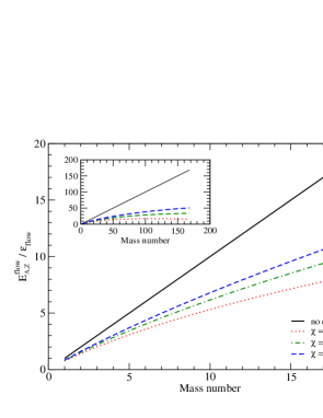
Figure 1: (Color online) $E^{\rm flow}_{A,Z}/\varepsilon_{\rm flow}$ as a function of the mass number, for $A_{0}=168$.

III Inclusion into the Statistical Multifragmentation Model

We briefly recall the main ingredients of the SMM. In it one assumes that the excited source undergoes a prompt statistical breakup, subject to strict mass, charge, and energy conservation Bondorf et al. (1985b); Sneppen (1987); Sneppen and Donangelo (1989),

$$A_{0}=\sum_{A,Z}N_{A,Z}A\;,\;\;\;Z_{0}=\sum_{A,Z}N_{A,Z}Z\;,$$ (9)

$$E_{0}^{\rm g.s.}+E^{*}=\frac{3}{5}\frac{Z_{0}^{2}e^{2}}{R}+\sum_{AZ}N_{A,Z}E_{A,Z}(T,V)\;.$$ (10)

Above, $E_{0}^{\rm g.s.}$ represents the ground state energy of the source, $E^{*}$ denotes the total excitation energy deposited into the system, and $e$ is the elementary charge. The fragment energies $E_{A,Z}$ have contributions from the translational motion, as well as from the nuclear bulk, surface, asymmetry, and Coulomb energies Aguiar et al. (2006). The latter, is calculated through the Wigner-Seitz approximation Bondorf et al. (1985b); Wigner and Seitz (1934). More specifically, $E_{A,Z}$ reads:

$$E_{A,Z}=-B_{A,Z}+E^{*}_{A,Z}+E^{C}_{A,Z}+\frac{3}{2}T+E^{\rm flow}_{A,Z}\;.$$ (11)

We stress that the effects discussed in this work are contained in the changes to the last term in the expression above, that were discussed in the previous section. The binding energy of the fragments, $B_{A,Z}$, is calculated using the prescription described in ref. Souza et al. (2003), whereas the remaining terms read:

$$E^{C}_{A,Z}=-C_{C}\frac{Z^{2}}{A^{1/3}}\left(\frac{1}{1+\chi}\right)^{1/3}\;,$$ (12)

$$E^{*}_{A,Z}=\frac{T^{2}}{\epsilon_{0}}A+\left(\beta(T)-T\frac{d\beta}{dT}-\beta_{0}\right)A^{2/3}\;,$$ (13)

and

$$\beta(T)=\left[\frac{T^{2}_{c}-T^{2}}{T^{2}_{c}+T^{2}}\right]^{5/4}\;.$$ (14)

We take for all parameters the same values used in ref. Tan et al. (2003), namely, a Coulomb parameter $C_{C}=0.720531$ MeV, bulk energy density parameter $\epsilon_{0}=16.0$ MeV, critical temperature $T_{c}=18.0$ MeV, and surface energy parameter $\beta_{0}=18.0$ MeV. One should notice that by adding the term associated with the Coulomb energy of the homogeneous sphere in Eq. (10) to the Coulomb contributions given by the fragments’ binding energies and Eq. (12), one obtains the Wigner-Seitz expression given in ref. Bondorf et al. (1985b). It is also worth mentioning that constraints on the center of mass motion are also imposed for each breakup partition, so that the total kinetic energy is given by Eq. (7).

The breakup temperature is determined, for each partition, by solving Eq. (10), so that it is strongly dependent on the partition mode. As the different terms in the sum appearing in Eq. (10) are affected in different ways according to the size of the fragments they represent, the temperature of the system will change appreciably from the value calculated without geometrical constraints.

The average value of a physical observable $O_{A,Z}$ is calculated through

$$\langle O_{A,Z}\rangle=\frac{\sum_{f}O_{A,Z}\exp\left[\sum_{\{A,Z\}_{f}}N_{A,Z}S_{A,Z}\right]}{\sum_{f}\exp\left[\sum_{\{A,Z\}_{f}}N_{A,Z}S_{A,Z}\right]}\;,$$ (15)

where the sum is performed over all possible partitions ${\{A,Z\}_{f}}$ of the nuclear system into fragments, and the entropy of fragment $(A,Z)$, $S_{A,Z}$, is calculated through the standard thermodynamic relation

$$S=-\frac{dF}{dT}$$ (16)

where $F$ is the Helmholtz free energy. Since it depends on the temperature of the fragmenting system, the weight of the corresponding mode is also influenced by the constraints just described. Ref. Tan et al. (2003) provides a detailed presentation on how empirical information is incorporated into $F$, and we refer the reader to that work for details. Except for the inclusion of the radial expansion, our SMM calculations follow the description of the Improved Statistical Multifragmentation Model (ISMM) presented in that work.

III.1 Deexcitation of the primary fragments

Since most excited fragments are detected after they have undergone secondary decay, we have used the Weisskopf treatment described in ref. Botvina et al. (1987) to estimate these effects on the fragment energy spectrum. In this approach, the probability that a compound nucleus, with total excitation energy $\varepsilon^{*}$, emits a fragment ($A$,$Z$), whose mass is $\mu_{A,Z}$, is proportional to

$$\Gamma_{A,Z}(\varepsilon^{*})=\sum_{i=0}^{n}\int_{0}^{\varepsilon^{*}-b_{A,Z}-\varepsilon_{A,Z}^{(i)}}f(\varepsilon)\,d\varepsilon\;,$$ (17)

where

$$f(\varepsilon)=\frac{g_{A,Z}^{(i)}\mu_{A,Z}\sigma_{A,Z}(\varepsilon)}{\pi^{2}\hbar^{3}}\frac{\rho_{R}(\varepsilon^{*}-b_{A,Z}-\varepsilon_{A,Z}^{(i)}-\varepsilon)}{\rho_{CN}(\varepsilon^{*})}\,\varepsilon\;.$$ (18)

In the expression above, $b_{A,Z}$ represents the separation energy, $g^{(i)}_{A,Z}$ denotes the spin degeneracy of the state $i$, $\sigma_{A,Z}$ is the cross-section of the inverse reaction, $\varepsilon_{A,Z}^{(i)}$ stands for the excitation energy of the emitted fragment, and $\rho(\varepsilon^{*})$ corresponds to the density of states of either the decaying nucleus (CN) or the residual fragment (R). We have used the same parameters of ref. Botvina et al. (1987), except for the binding energies and the level densities. The former are the same used in our SMM calculations, whereas the latter are given by the standard Fermi-gas expression $\langle\varepsilon^{*}\rangle/A=aT^{2}$, but the excitation energy and the breakup temperature are taken as the average values obtained through Eq. (15) for each primordial species. Therefore, the density of states

$$\rho(\varepsilon^{*})\propto\exp\left(2\sqrt{a\varepsilon^{*}}\right)$$ (19)

has a different level density parameter $a$ for distinct primary fragment species. This ensures consistency with the population of the excited states in SMM and in the secondary decay treatment.

The final kinetic energy spectrum is generated by a Monte Carlo sample of the possible decay channels of the primary distribution. More specifically, the excitation energy of a given primordial fragment is selected with probability

$$P_{E}(\varepsilon^{*})\propto\exp(-\varepsilon^{*}/T)\rho_{CN}(\varepsilon*)\;.$$ (20)

The thermal velocity of the decaying fragment is then assigned according to the Boltzmann distribution.

The radial expansion is incorporated by adding to the velocity a contribution given by Eq. (4). For consistency, the position of the fragment is uniformly sampled within a spherical volume of radius $R$, which is equal to the breakup volume of the system. We also impose the constraint that the fragment must lie entirely inside it. The contribution to the kinetic energy due to the Coulomb interaction is estimated by considering the repulsion between the fragment and the remaining part of the system. We simply assume that the fragment with atomic number $Z_{f}$ is situated inside a sphere of charge $(Z_{0}-Z_{f})e$, homogeneously distributed within its volume. The recoil of this core is taken into account when the corresponding boost associated with this binary repulsion is added to the fragment’s velocity.

The selection of a specific channel is made with probability

$$P_{A,Z}(\varepsilon^{*})=\frac{\Gamma_{A,Z}(\varepsilon^{*})}{\sum_{\{A,Z\}}\Gamma_{A,Z}(\varepsilon^{*})}\;,$$ (21)

where the sum runs over all possible decay channels. We have considered the emission of all nuclei from $A=1$ to $A=10$.

For the selected deexcitation mode, the relative kinetic energy of the products $\epsilon\leq\varepsilon^{*}-b_{A,Z}-\varepsilon_{A,Z}^{(i)}$ is sampled with weight proportional to Eq. (18). Their velocities, in the rest frame of the decaying fragment, are determined by energy and momentum conservation. The excitation energy of the residue is then obtained by energy conservation and it reads $\varepsilon^{*}_{R}=\varepsilon^{*}-b_{A,Z}-\varepsilon_{A,Z}^{(i)}-\varepsilon$. The decay chain is followed until the remnant fragment has a negligible amount of excitation energy, i.e. it cannot decay by particle emition.

This Monte Carlo sample is repeated $10^{5}$ times for each primary species. In the end, the multiplicities are weighed proportionally to the multiplicity of the primordial fragments.

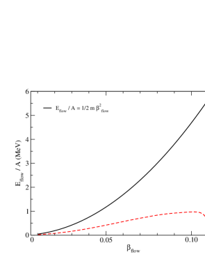
Figure 2: (Color online) Average flow energy as a function of the average flow velocity. The full curve illustrates the results without inclusion of geometrical constraints whereas the dashed one corresponds to those with their inclusion. For additional details see the text.

IV Results

To investigate the effects of the collective radial expansion in SMM, we study the $A_{0}=168$ $Z_{0}=75$ system, at a fixed breakup density. In Fig. 2, we show the average flow energy, $E_{\rm flow}$, calculated through Eqs. (8) and (15), as a function of the radial velocity $\beta_{\rm flow}$ (dashed line), in a case where the system expanded to three times its volume at normal nuclear density, i.e. $\chi=2$. The total available excitation energy of the system was taken to be $E^{*}/A=6$ MeV. Comparison with the standard unconstrained values, represented in this picture by the full line, demonstrates that the inclusion of the geometric constraints dramatically suppresses the amount of energy which may be actually used in the radial collective expansion. One also observes that the flow energy reaches a maximum value, of approximately $E_{\rm flow}/A=1$ MeV at a value of $\beta_{\rm flow}=\beta_{\rm max}\approx 0.105$ close to the maximum possible (when all the energy available would appear as radial flow), and then drops to zero as $\beta_{\rm flow}$ increases further. This behaviour may be understood as a consequence of the fact that the total entropy of the system diminishes as more and more energy is stored into organized motion, reducing the accessible phase space associated with partitions leading to large flow energy values. Since the expansion velocity was taken to have a fixed value for all partitions, those which include large fragments, and consequently have smaller fragment multiplicities, are clearly favored, since they lead to smaller flow energies.

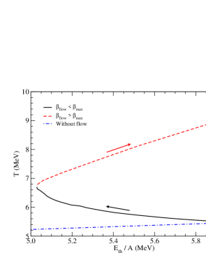
Figure 3: (Color online) Average breakup temperature as a function of the average thermal energy. The dash-dotted curve illustrates the results obtained when geometrical constraints are not included. The full and dashed curve are the results when these constraints are included: the full (dashed) curve corresponds to velocity flow values below (above) the one leading to a maximum flow energy, as depicted in fig. 2. The arrows indicate the direction in which the radial velocity increases.

The changes on the preferred partitions reflect themselves on many observables, such as the breakup temperature. Indeed, SMM calculations at fixed breakup volume clearly show that the breakup temperature becomes smaller if one simply removes the corresponding amount of flow energy from the total excitation energy (see, for instance, Souza et al. (2004) and references therein). This is illustrated by the dotted-dashed line in Fig. 3, which displays the breakup temperature as a function of the thermal excitation energy, in the case where geometrical constraints are disregarded. On the other hand, the constraints associated with the collective motion causes the breakup temperature, at a fixed total available excitation energy, to rise instead of diminishing, as is also shown in this picture. In this case, the thermal energy is defined as the difference between the total available excitation energy and the average flow energy, i.e., $E_{\rm th}=E^{*}-E_{\rm flow}$. This behavior may be explained by the reduction of the fragment multiplicity, which leads to larger fragments, moving with less flow energy. The requirement of energy conservation, Eq. (10), then leads to a higher temperature than when the constraints are not included.

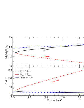
Figure 4: (Color online) Average primary multiplicity (upper panel) and average mass number (lower panel) of fragments as a function of the thermal excitation energy. The curves correspond to the same cases illustrated in fig.3.

The changes on the primary fragment multiplicity and on their average fragment size are shown in Fig. 4 as a function of the thermal excitation energy. As in the previous plot, the dashed-dotted line represents the results obtained without geometrical constraints. The inclusion of these constraints causes the fragment multiplicity to drop down as the thermal excitation decreases, before the average flow energy reaches its maximum value, i.e., for $\beta_{\rm flow}<\beta_{\rm max}$. Then, for $\beta_{\rm flow}>\beta_{\rm max}$, it keeps going down while the thermal energy increases until it reaches the smallest possible value $M_{f}=1$. As expected, the opposite trend is observed for the average fragment size.

In spite of the important changes on the observables, the energy spectrum of the particles still exhibits a shape which is similar to that expected without constraints associated with the finite fragment sizes. Indeed, the circles in Fig. 5 represent the average kinetic energy of the primary fragments versus their atomic numbers. The simulation has been carried out for $E^{*}/A=6.0$ MeV, $\beta_{\rm flow}=\sqrt{2\varepsilon_{\rm flow}/m}$, and $\varepsilon_{\rm flow}=2.0$ MeV. As shown in that figure, the results can be fitted by the linear function $E_{Z}=12.3+1.4Z$ MeV. If the energy spectrum were interpreted disregarding the geometric constraints, and one wrote $E_{Z}=\frac{3}{2}T+\varepsilon_{\rm flow}2Z$, comparison with the fit would lead to $T=8.2$ MeV and $\varepsilon_{\rm flow}=0.7$ MeV. However, the simulation gives $T=5.9$ MeV and, as already mentioned, the expansion velocity corresponds to $\varepsilon_{\rm flow}=2.0$ MeV. Therefore, the neglect of geometric constraints may lead to important uncertainties in the interpretation of the experimental observations.

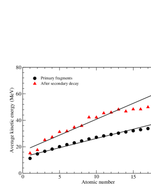
Figure 5: (Color online) Average frament kinetic energy as a function of the fragments’ atomic numbers. The lines correspond to a linear fit of the results.

In order to investigate the influence of the effects associated with the decay of the hot primary fragments on the energy spectrum, we have employed the deexcitation treatment presented in sect. III.1. The kinetic energy of the fragments after secondary decay is depicted in Fig. 5 by the triangles. As may be noticed, the slope of the spectrum increases appreciably and one may adjust a linear function to reproduce its main trends. Then, one finds $E_{Z}\approx 16.8+2.4Z$ MeV. One sees that the Coulomb repulsion among the fragments appreciably affects the slope of the distribution, besides the overall enhancement of the fragment’s kinetic energy. Nevertheless, the slope is still much smaller than what would be given by radial flow alone if the geometric constraints were not taken into account. In spite of the great simplifications adopted in our deexcitation treatment, we believe that the main effects are included in it, so that more refined decay schemes should not change our conclusions significantly. Therefore, our results suggest that the consistent treatment of the geometrical constraints are very important in interpreting the experimental observations.

V Concluding remarks

We have investigated the effects of the inclusion of geometric constraints due to the finite size of fragments in multifragmentation at a fixed breakup volume. Our results show that the inclusion of these constraints in SMM lead to qualitative different conclusions on the behavior of many physical observables as the system undergoes a radial collective expansion. In particular, our results suggest that radial flow alone should not be able to explain a very large increase of the fragments kinetic energy as a function of the atomic number. Indeed, the simulations presented here show that, for a fixed total excitation energy, the amount of energy stored in the radial expansion is strongly suppressed. As a consequence, other mechanisms should be considered in order to explain the slopes observed experimentally in the energy spectra of the fragments. Thus, we believe that interpretations based on statistical calculations in which energy flow is simply removed from the total energy should be reviewed.