SUPERSTATISTICS OF BROWNIAN MOTION: A COMPARATIVE STUDY

Abstract

The dynamics of temperature fluctuations of a gas of Brownian particles in local equilibrium with a nonequilibrium heat bath, are described using an approach consistent with Boltzmann-Gibbs statistics ($BG$). We use mesoscopic nonequilibrium thermodynamics ($MNET$) to derive a Fokker-Planck equation for the probability distribution in phase space including the local intensive variables fluctuations. We contract the description to obtain an effective probability distribution ($EPD$) from which the mass density, van Hove’s function and the dynamic structure factor of the system are obtained. The main result is to show that in the long time limit the $EPD$ exhibits a similar behavior as the superstatistics distribution of nonextensive statistical mechanics ($NESM$), therfore implying that the coarse-graining procedure is responsible for the so called nonextensive effects.

I Introduction

The existence of fluctuations of intensive parameters, such as the inverse temperature, the chemical potential, the pressure or the energy dissipation rate in a turbulent fluid, is a common feature in a variety of physical systems in nonequilibrium states ausloos , beck3 , beck1 , fluct-friction . However, the theoretical description of these fluctuations is well beyond the range of applicability of the theory of fluctuations as developed by Onsager and Machlup onsager and subsequent generalization by Fox and Uhlenbeck fox , and others ortiz . This is essentially due to the fact that these theories are restricted to describe the dynamics of fluctuations of extensive state variables only.

One of the most used methods to deal with intensive variable fluctuations is the superstatistics approach of $NESM$, tsallis , abe , beck2 , cohen1 . This theory claims that a proper description of these fluctuations for systems with a sufficiently complex dynamics, demands the introduction of a more general statistics — Tsallis statistics ($TS$) — than the usual Boltzmann-Gibbs statistics ($BG$). Furthermore, according to Refs. beck1 , cohen1 , $TS$ is only one of many more general statistics — superstatistics — that can deal with the physical situations mentioned above. An important and simple system where these issues have been explored is Brownian motion in the presence of inverse temperature fluctuations beck1 . In this reference the fluctuations of the intensive parameter $1/T$ are not described as a fully time-dependent phenomena, rather only their statistics is taken into account and postulated without a physical justification, by assuming that if $\beta$ is a $\chi^{2}$ distributed random variable. By averaging over its (static) statistical distribution this model generates $TS$ for $v$ for a stationary state. On this basis, it is suggested that $BG$ is no longer capable of describing correctly this physical situation and that a new statistics ($TS$) is required.

The main motivation of the present work is to consider inverse temperature fluctuations in the same model as in Ref. beck1 , but describing their dynamics in terms of a stochastic process, and following their time evolution towards equilibrium. By using $MNET$ mazur , pnas , reguera , the time evolution of the nonequilibrium state is described in the phase space of the particles, including the local intensive fluctuations as state variables, by means of a Fokker-Planck equation ($FPE$). In the diffusion limit this description leads in a natural way to a stochastic Smoluchowski equation for the contracted distribution function. By following a method introduced by van Kampen to solve multiplicative stochastic equations van kampen , we derive an equation for the effective distribution function ($EDF$), which still contains all the effects produced by the induced (intensive) fluctuations. The long time limit behavior of the $EDF$ as a function of position, is similar to the behavior found in $NESM$ for the so-called superstatistical distribution. In this way, our approach shows to be an alternative way to describe the dynamics of intensive fluctuations consistently with $BG$.

We will proceed as follows. In Section 2, we present a derivation of the $FPE$, ivan1 . In Section 3 we model the temperature fluctuations by means of a stochastic process and after contracting the $FPE$, we derive a stochastic multiplicative Smoluchowski equation ($MSE$), valid for an arbitrary stochastic dynamics of its coefficients. We conclude this section by deriving from it a deterministic equation for the $EDF$. The solution of this equation allows us to calculate the van Hoveś function and the dynamic structure factor of the gas, which are obtained in Section 4. In Section 5 we show that when the long time limit of the $EDF$ is evaluated as a function of the position, the contraction procedure and the non-Gaussian corrections introduced by solving the $MSE$, yield a behavior which reproduce the one proposed by $NESM$ for the same model. We conclude with a discussion of the results of Section 5.

II Smoluchowski equation

Following Ref. beck1 , we consider a driven nonequilibrium system composed of regions (cells) of size $l$ where fluctuations of $1/T$ may occur beck2 . In this model system, it is assumed that the local temperature of a cell changes in a time scale, $\tau$, much larger than the relaxation time a region needs to reach local equilibrium. Within each cell a spherical test particle of radius $a$ and mass unity, performs Brownian motion and then moves to another cell. Its velocity may be described by a linear Langevin equation of the form

$$\frac{dv}{dt}=-\gamma v+\sigma L(t),$$ (1)

where $\gamma>0$ is a friction constant, $L(t)$ is Gaussian white noise and $\sigma$ describes the strength of the noise. For this model the inverse temperature $\beta=\gamma/\sigma^{2}$ is no longer constant, but fluctuates in space and time on the scales $l$ and $\tau$, respectively. As a result, Brownian motion takes place on two time scales, one related to the dissipation of the kinetic energy through the Stokes friction coefficient $\gamma=6\pi\eta a$, where $\eta$ is the shear viscosity of the host fluid, and the second one is associated with the presence of temperature fluctuations induced on the whole system by an external agent. These fluctuations originate in the environment of the Brownian particles (heat bath) and in some cases may therefore possess a complex dynamics.

In local equilibrium, the probability of finding a Brownian particle in position $\vec{r}$ with instantaneous velocity $\vec{u}$ in the presence of the temperature fluctuations $\delta T$, is described by the local equilibrium probability density $P_{le}(\vec{r},\vec{u};\delta T)$. This quantity may be determined through the calculation of the amount of work exerted on a particle at temperature $T$ in the presence of an external potential $\phi(\vec{r})$ and of a local temperature fluctuation $\delta T(t)\equiv T-T_{B}$, where $T_{B}$ is the temperature of the bath mazur , ivan1 , de groot , landau sp . If the spontaneous thermal (equilibrium) fluctuations $\Delta T$ are such that $\Delta T\ll\delta T$, the expression for $P_{le}$ is ivan1

$$P_{le}(u)=P_{0}e^{-\frac{m}{2k_{B}T}\left(u^{2}+\phi\right)}e^{-\frac{mc_{v}}{k_{B}}\frac{\left(\Delta T\right)^{2}}{TT_{B}}},$$ (2)

where $m$ is the mass of the particle, $c_{v}\equiv\partial e/\partial T_{B}$ is the specific heat at constant volume, $e$ is the internal energy density and where the density fluctuations of the heat bath have been neglected .

The dynamics of the Brownian particle may be described through the nonequilibrium probability density $P(\vec{r},\vec{u},t;\delta T)$. The time evolution equation for this quantity is derived from the entropy production $\partial\Delta s(t)/\partial t$, where the nonequilibrium entropy increment $\Delta s(t)$ is given by the generalized Gibbs entropy postulate

$$\Delta s(t)=-k_{B}\int P\ln\frac{P}{P_{le}}d\vec{r}d\vec{u}.$$ (3)

Since the probability conservation is expressed through the continuity equation

$$\frac{\partial P}{\partial t}=-\frac{\partial}{\partial\vec{r}}\cdot\left(\vec{u}P\right)-\frac{\partial}{\partial\vec{u}}\cdot\left(\vec{V}_{\vec{u}}P\right),$$ (4)

from Eqs. (2), (3) and (4) and by using the boundary conditions for the fluxes, we get an expression for the entropy production where fluxes and forces may be clearly identified, pnas , reguera , ivan1 . By assuming linear relationships between fluxes and forces we finally arrive at the Fokker-Planck equation

$$\frac{\partial}{\partial t}P+\frac{\partial}{\partial\vec{r}}\cdot\left(\vec{u}P\right)=\frac{\partial}{\partial\vec{u}}\cdot\left[\left(\beta\vec{u}+\frac{\partial\phi}{\partial\vec{r}}\right)P+\frac{k_{B}T}{m}\beta\frac{\partial P}{\partial\vec{u}}\right],$$ (5)

where we have taken the coupling coefficient for the external force ${\partial\phi}/{\partial\vec{r}}$ as one, in accordance with the phenomenological description we are using nonmarkov , adelman . It should be pointed out that in arriving at Eq. (5) we have neglected the contribution arising from the usual thermal fluctuations in Eq. (2), in accordance with the assumption $\Delta T\ll\delta T$.

The Smoluchowski equation for the reduced probability distribution $\rho(\vec{r},t)\equiv\int Pd\vec{u}$ can be derived in the limit of long times, by calculating the evolution equations for the first three moments of $P$ over $\vec{u}$-space, namely, the mass density $\rho(\vec{r},t)\equiv\int Pd\vec{u}$, the momentum density $\rho\vec{v}(\vec{r},t)$ and the stress tensor density. For sufficiently long times, one may assume that the stresses and momenta have relaxed, and by combining them we obtain a constitutive relation for the diffusion flow (see Ref. ivan1 for details). After substitution of this constitutive relation into the continuity equation we are lead to

$$\frac{\partial\rho}{\partial t}=\beta^{-1}\frac{\partial}{\partial\vec{r}}\cdot\left(\rho\frac{\partial\phi}{\partial\vec{r}}\right)+D\frac{\partial^{2}\rho}{\partial\vec{r}^{2}},$$ (6)

where in the last term we have taken into account that $T=T_{B}+\delta T$ and Eq. (6) contains the diffusion coefficient

$$D\equiv\left({k_{B}T_{B}}/{m\beta}\right)\left(1+{\delta T}/{T_{B}}\right),$$ (7)

which explicitly incorporates the effects of the externally induced fluctuations on the temperature of the bath. It is convenient to stress that equations similar to (6) have been previously derived in the context of slow relaxation systems such as supercooled colloidal suspensions and granular systems, among others slow , jpcm . However, in these cases, the temperature $T$ was assumed to be a decaying function of time, related with an activated process which controls the relaxation. In contrast, in the present work we considered the more general situation where the temperature fluctuation $\delta T(t)$ is assumed to be a stochastic process, which converts Eq. (6) into a multiplicative stochastic partial differential equation ($MSE$).

III Effective probability distribution

With the purpose of obtaining macroscopic local variables which eventually may be measured, such as the dynamic structure factor, the van Hove’s function, or the local mass density, we contract the description over velocities and $\delta T(t)$. To this end we define the $EDF$ as

$$\langle\rho(\vec{r},t)\rangle\equiv\int P(\vec{r},\vec{u},t;\delta T)d\vec{u}d(\delta T).$$ (8)

A time evolution equation for the $EDF$ is obtained by deriving an approximate solution of Eq. (6) through the use of a method proposed by van Kampen which yields an equation for the average $\langle\rho(\vec{r},t)\rangle$, van kampen . This approximation takes the form of a series expansion in powers of the Kubo number, $\alpha\tau_{c}$, which is assumed to be small. Here $\alpha$ is a parameter measuring the magnitude of the fluctuations in the coefficients of Eq. (6) and $\tau_{c}$ denotes their finite autocorrelation time van kampen .

This derivation may be easily generalized to consider the case where the particle is also under the influence of a harmonic force derived form the potential $\phi=\omega_{0}^{2}\vec{r}^{2}/2$, where $\omega_{0}$ denotes its characteristic frequency. Let us assume that $\delta T(t)$ is of the form

$$\delta T(t)/T_{B}=\alpha\zeta(t),$$ (9)

with $\zeta(t)$ is an arbitrary stochastic process with zero mean and autocorrelation

$$\langle\zeta(t-\tau)\zeta(t)\rangle=\Pi(\tau).$$ (10)

Accordingly, we recast Eq. (6) as the following multiplicative stochastic equation for $\rho(\vec{x},t)$,

$$\frac{\partial\rho}{\partial\tilde{t}}=\tilde{\nabla}\cdot(\rho\vec{x})+\Gamma\tilde{\nabla}^{2}\rho+\alpha\Gamma\zeta(\tilde{t})\tilde{\nabla}^{2}\rho.$$ (11)

where for convenience we have introduced the dimensionless variables $\vec{x}\equiv a^{-1}\vec{r}$, $\tilde{t}\equiv\omega^{2}\beta^{-1}t$ and the operator $\tilde{\nabla}$ indicates differentiation with respect to $\vec{x}$. The parameter $\Gamma\equiv k_{B}T_{B}/ma^{2}\omega^{2}$ is the ratio between the thermal energy of the bath and the energy supplied by the external source, while maintaining the nonequilibrium state. By taking the Fourier transform over the space variables, Eq. (11) is rewritten as

$$\frac{\partial}{\partial\tilde{t}}\hat{\rho}(\vec{q},t)=-\vec{q}\cdot\frac{\partial\hat{\rho}}{\partial\vec{q}}-\Gamma\left(q^{2}+\alpha\zeta(\tilde{t})q^{2}\right)\hat{\rho},$$ (12)

where the caret stands for the Fourier transform of a quantity.

To implement van Kampen’s method explicitly, it is convenient to identify the systematic and stochastic operators on the right hand side ($r.h.s.$) of Eq. (12)  as

$$A_{0}\equiv-\vec{q}\cdot\frac{\partial}{\partial\vec{q}}-\Gamma q^{2},$$ (13)

and

$$A_{1}(t)\equiv-\alpha\Gamma\zeta(t)q^{2}.$$ (14)

Following van Kampen’s method for times satisfying $\tau_{c}\ll t\ll\alpha^{-1}$, the average $\langle\hat{\rho}(\vec{q},t)\rangle$ over the realizations of $\zeta(t)$ obeys by itself the approximate non-stochastic equation

$$\frac{\partial\langle\hat{\rho}\rangle}{\partial\tilde{t}}=\left[A_{0}+\alpha^{2}\int_{0}^{\infty}d\tau\langle A_{1}(\tilde{t})e^{\tau A_{0}}A_{1}(\tilde{t}-\tau)e^{-\tau A_{0}}\rangle\right]\langle\hat{\rho}\rangle.$$ (15)

After evaluating the action of the operators $A_{0}$ and $A_{1}$, Eq. (15) may be rewritten in the more compact form

$$\frac{\partial\langle\hat{\rho}\rangle}{\partial\tilde{t}}=-\left(\vec{q}\cdot\frac{\partial}{\partial\vec{q}}+q^{2}\Gamma\right)\langle\hat{\rho}\rangle+\Gamma^{2}\alpha^{2}C(\tilde{t})q^{4}\langle\hat{\rho}\rangle,$$ (16)

where $C(\tilde{t})$ is defined in terms of the autocorrelation of the noise

$$C(\tilde{t})\equiv\int_{0}^{\infty}d\tau\langle\zeta(\tilde{t})\zeta(\tilde{t}-\tau)\rangle,$$ (17)

which is so far arbitrary. Note that the second term on the $r.h.s.$ of Eq. (16) incorporates in an average way the effects of the temperature fluctuations on the dynamics of the system. It also introduces time dependent non-Gaussian corrections and gives rise to non-stationary effects on the dynamics.

If for simplicity in the discussion we consider the special case where the temperature fluctuations may be represented by a stationary stochastic process, $C(t)=C(0)\equiv C_{0}$, and the steady state solution of Eq. (16) reduces to

$$\langle\hat{\rho}(q)\rangle=\rho_{0}\,e^{-\frac{\Gamma}{2}q^{2}}\,e^{\frac{\alpha^{2}\Gamma^{2}C_{0}}{4}q^{4}},$$ (18)

where $\rho_{0}$ is a normalization factor. To comply with the approximation of van Kampen’s method, this solution is expanded up to order $\alpha^{2}$ and then the inverse Fourier transform of the resulting expression is taken. This leads to a solution which contains explicit non-Gaussian corrections to the steady state distribution function,

$$\langle\rho(x)\rangle=\frac{\rho_{0}}{\sqrt{2\pi\Gamma}}e^{-\frac{1}{2\Gamma}x^{2}}\left[1+\frac{1}{4}\alpha^{2}\Gamma^{2}C_{0}f(x)\right],$$ (19)

with $f(x)=\Gamma^{-2}x^{4}-6\Gamma^{-1}x^{2}+3$. For future convenience we expand the above expression in a Taylor series in $x$,

$$\langle\rho(x)\rangle_{s}\simeq\frac{\rho_{0}(2\pi\Gamma)^{-1/2}}{1+\frac{x^{2}}{2\Gamma}+...}\left[1+\frac{1}{4}\alpha^{2}C_{0}f(x)\right].$$ (20)

Notice that a different (but similar) expansion can be carried out in terms of the well known formula $e^{-y}\simeq\left(1-\frac{y}{b}\right)^{b}$, which leads to

$$\langle\rho(x)\rangle_{e}\simeq\rho_{0}(2\pi\Gamma)^{-1/2}\left(1-\frac{x^{2}}{2\Gamma b}\right)^{b}\left[1+\frac{1}{4}\alpha^{2}C_{0}f(x)\right].$$ (21)

IV van Hove’s function and structure factor

Owing to its direct relation with experimental techniques, we shall now calculate the density correlation function boon . The space Fourier transform of this quantity is the van Hove function $\hat{F}$,

$$\hat{F}(\vec{q},\tilde{t})\equiv\langle\rho(\vec{q},\tilde{t})\rho(\vec{q}_{0},\tilde{t}_{0})\rangle,$$ (22)

where $\vec{q}_{0}$ will be considered as a reference wave vector, $\tilde{t}_{0}$ is an initial time and, as before, the bracket $\langle..\,\rangle$ denotes an average over the realizations of the external noise $\zeta(t)$.

The time evolution equation of this quantity is obtained by multiplying Eq. (12) by $\hat{\rho}(\vec{q}_{0},\tilde{t}_{0})$ and using Eqs. (13-14), yielding

$$\frac{\partial}{\partial\tilde{t}}\hat{F}^{\ast}(\vec{q},t)=\left[A_{0}+A_{1}(\tilde{t})\right]\hat{F}^{\ast}(\vec{q},\tilde{t}),$$ (23)

where we have used the notation $\hat{F}^{\ast}(\vec{q},t)\equiv\left\langle\rho(\vec{q},t)\rho(\vec{q}_{0},t_{0})\right\rangle$. Since Eq. (23) is of the same type as Eq. (12), van Kampen’s method also leads to the evolution equation

$$\frac{\partial\hat{F}}{\partial\tilde{t}}=-\left(\vec{q}\cdot\frac{\partial}{\partial\vec{q}}+q^{2}\Gamma\right)\hat{F}+\Gamma^{2}\alpha^{2}C(\tilde{t})q^{4}\hat{F},$$ (24)

for $\hat{F}(\vec{q},\tilde{t})$ defined by Eq. (22). Again, for the special case where the temperature fluctuations may be represented by a stationary stochastic process, the steady state solution of Eq. (24) has the form (18),

$$\hat{F}_{s}(\vec{q})=e^{-\frac{\Gamma}{2}q^{2}}\,e^{\frac{\alpha^{2}\Gamma^{2}C_{0}}{4}q^{4}}.$$ (25)

Furthermore, using this result and the fact that Eq. (24) is a linear hyperbolic partial differential equation which can be solved by using the method of the characteristics, we arrive at the following time dependent solution of Eq. (24)

$$\hat{F}(\vec{q},t)\simeq\left(1+\frac{\alpha^{2}\Gamma^{2}C_{0}}{4}q^{4}\right)e^{-\frac{\Gamma}{2}q^{2}-z^{2}(q,t)}.$$ (26)

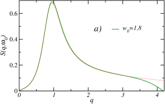
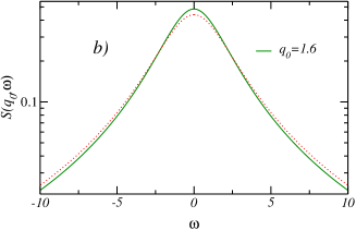
Again, we have only retained terms up to order $\alpha^{2}$ to be consistent with the approximation used in van Kampen’s method, and we have used the scaling variable $z(q,t)\equiv t-\ln|q|$. Since the $z$ dependence of the solution of Eq. (24) should decay with $z$, we have chosen the form $e^{-z^{2}}$. Equation (26) actually imply that $F(\vec{q},t)$ has a similar behavior as the probability density $\left\langle\rho(\vec{q},t)\right\rangle$. Figures 1a and 1b show a plot of $\hat{F}(\vec{q},t)$ as a function of $\vec{q}$ and $t$ for fixed values of $t$ and $\vec{q}$, respectively. They show that the presence of temperature fluctuations indeed modifies the behavior of $F(\vec{q},t)$ with respect to the case where no intensive fluctuations are present. We have expressed the wave vector as $\vec{q}\equiv q\widehat{k}$, where $\widehat{k}$ is a unit vector in the direction of $\vec{q}$. It is important to point out that, in order to represent Eq. (26) by Figs. 1 (and Eq. (28) through Figs. 2), we have chosen values for the coefficients $\Gamma$, $\alpha$ and $C_{0}$ consistently with the approximations introduced in the previous section. This means that the physical parameters ($T$, $\omega$, $\beta$) characterizing the system are determined.

Figure 1: a) $\widehat{F}(\vec{q},t)$ vs. $q$. The red lines correspond to the case without temperature fluctuations. The remaining lines green to blue, are obtained from Eq. (26) for $t=0.1$, $0.3$, $0.6$, $0.9$, respectively. b) $F(\vec{q},t)$ vs. $t$ for fixed values of $q=0.5$ (green) and $q=0.6$ (blue). The value of the parameters are $C_{0}=0.8$, $\Gamma=1$ and $\alpha=0.8$.

Fig. 1a shows that the external fluctuations induce significant corrections to $F(\vec{q},t)$ for values of $q>0.5$ for various fixed time values (see caption). The red lines correspond to the case without (intensive) temperature fluctuations, whereas the green to blue lines correspond to the case when these fluctuations are present. This figure implies that intensive temperature fluctuations slow down the decay of the density-density correlation function. On the other hand, Fig. 1b shows the corrections corresponding to the time dependence of van Hove’s function for $q=0.5$ (green) and $q=0.6$ (blue).

The Fourier’s transform of $\hat{F}(\vec{q},t)$ with respect to time defines the dynamic structure factor $\hat{S}(q,\omega)$,

$$\tilde{S}(q,\omega)=\frac{\hat{S}(q,\omega)}{S(q_{0},0)}=e^{i\omega\ln|q|-\frac{\Gamma}{2}q^{2}(1-\frac{\Gamma}{2}\alpha^{2}C_{0}q^{2})}.$$ (27)

Expanding this function up to first order in its argument, we arrive at

$$\tilde{S}(q,\omega)=G^{-1}(q,\omega)\left[1+\frac{\Gamma}{2}q^{2}(1-\frac{\Gamma}{2}\alpha^{2}C_{0}q^{2})\right],$$ (28)

where we have defined the inverse propagator

$$G^{-1}(q,\omega)\equiv\left[1+\frac{\Gamma}{2}q^{2}(1-\frac{\Gamma}{2}\alpha^{2}C_{0}q^{2})\right]^{2}+\left[\omega\ln|q^{2}|\right]^{2}.$$ (29)

Figure 2: a) $S(\vec{q},\omega)$ vs. $q$ for $\omega=1.8$ and b) $S(\vec{q},\omega)$ vs. $q$ for $q=1.6$. The red lines correspond to the case without temperature fluctuations whereas the green line include temperature fluctuations for $\alpha=0.8$, $C_{0}=0.8$ and $\Gamma=1$.

Eq. (28) explicitly shows that the presence of the intensive fluctuations indeed modify the behavior of the structure factor, as expected. The presence of powers of $q$ higher than $q^{2}$ suggests the existence of long-range correlations induced by intensive temperature fluctuations. In Figs. 2 we show the projections of the structure factor for fixed $q$ (Fig. 2a) and for fixed $\omega$ (Fig. 2b). Note that in Fig. 2b the green line is $\sim 1.2$-times larger than the red one for $\omega=0$. If $\omega\sim 2.5$ the green line has the same value as the red one and for $\omega\simeq 10$ the green line is $\sim 0.6$-times larger than the red one. Clearly, the presence of temperature fluctuations induces an anomalous behavior of the structure factor in the $\omega$-fixed plane. It should be pointed out that in this case, our results are only valid for $q<(c\alpha^{2}\Gamma)^{-1/2}(1+\sqrt{1+4c\alpha^{2}})$.

V Comparison with Superstatistics

In order to compare the results obtained in this work with those derived from the superstatistics approach reported in Refs. beck2 ; beck3 , we recall that in these references it is argued that the stochastic differential equation (1) with a $\chi^{2}$ distributed $\beta$, gives rise to the generalized canonical distributions of $NESM$ tsallis ,

$$\rho_{NESM}(x)=\left[1+\frac{\beta_{0}}{n}x^{2}\right]^{-\frac{n+1}{2}},$$ (30)

where $n$ is a positive integer and $\beta_{0}=\left\langle\beta\right\rangle$. Eq. (30) contains two free parameters ($\beta_{0}$ and $n$) that must be fitted in order to represent the function. Both parameters arise from the initial assumption that the inverse temperature is a $\chi^{2}$ distributed variable; however, the physical meaning of these parameters remains unknown. Moreover, it is interesting to notice that the form of Eq. (30) is independent of the nature of the variable of interest. For example, in Ref. beck2 , a similar expression (with one more parameter) is used in order to fit the distribution of velocities in a fluid undergoing stationary turbulence.

Figure 3: The blue line represents the stationary $EDF$ as given by Eq. (20) vs. $x$, for $n=18$ and with $\alpha=0.5$, $C_{0}=0.25$, $\Gamma=0.13$. The green line represents an expansion of  the exponential in the stationary $EDF$ by using Eq. (21) with $b=8$ and $\alpha=0.02$, $C_{0}=0.12$ and $\Gamma=0.12$.

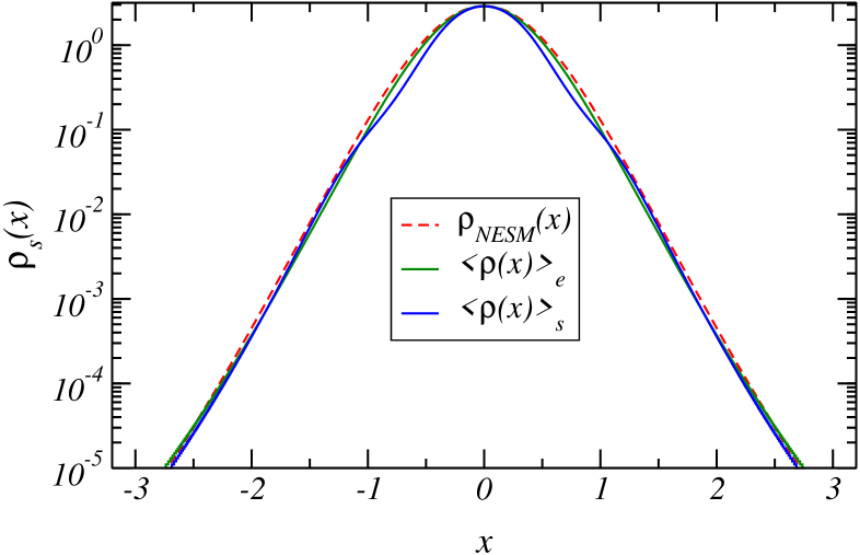
Figure 3 shows a comparison between our steady state distribution function, as given by Eq. (20) (blue line), and the above expression for $\rho_{NESM}(x)$ (red line), for different values of the parameter $n$. The green line corresponds to Eq. (21). The difference between these curves lies in the fact that the superstatistical method beck2 , essentially analyzes the statistics of a system in local equilibrium, and considers the fluctuations of the intensive parameters to be of a static nature. On the contrary, Eq. (18) represents the long time limit of the dynamic analysis that has taken into account the (irreversible) time dependent process associated with the intensive fluctuations. Moreover, the parameters entering into Eq. (20) are determined by the nature of the system and must satisfy the conditions imposed by the approximations of Sec. III, ($\tau_{c}\alpha\ll 1$). In order to find a good comparison between the red and blue lines, we have chosen the adequate order of the polynomial arising from the Taylor expansion of the exponential.

It should be pointed out that in all cases the value of $\Gamma$ controls the form of the peak, whereas the strength of the noise $\alpha$ and the noise correlation $C_{0}$ control the tail of the distribution. The larger the values of $\alpha$ and $C_{0}$, the larger the inflexion intermediate values of $x$.

VI Discussion

In this work we have analyzed the problem of Brownian motion introduced in Ref. beck2 by using a mesoscopic approach ($MNET)$. The time evolution of the nonequilibrium state of the system is described by means of a Fokker-Planck equation for the probability distribution in the phase space of the particles including local intensive parameter fluctuations. The basic difference with the point of view adopted in beck2 is that the dynamics of the (intensive) temperature fluctuations is explicitly taken into account by representing them as a stochastic process.

An essential element in our approach is the contraction of the above description which yields a stochastic multiplicative Smoluchowski equation for the (local) reduced probability density. The (approximate) solution of this equation yields a deterministic equation for an effective probability distribution ($EPD$) valid for an arbitrary stochastic dynamics of the random coefficients. As a consequence, we calculated two measurable quantities, the van Hove’s function and the dynamic structure factor of the system; however, we are not aware of any experimental results to compare with these predictions of our model.

The most important conclusion that arises from our approach is that the long time limit of our $EPD$ as a function of position, exhibits a similar behavior to the so called superstatistical distribution in nonextensive statistical mechanics ($NESM$), beck2 . This result shows that the dynamics of intensive parameter fluctuations is fully consistent with Boltzmann-Gibbs statistics. The coarse-graining procedure and the time dependent non-Gaussian corrections introduced in solving the $MSE$, gave rise to non-stationary effects on the dynamics and generated those features of the $EPD$ which are usually identified with the so called nonextensive effects of $NESM$.

Our approach can be used for both, stationary and non-stationary fluctuations of the intensive parameters. However, it should be stressed that our approach and conclusions are only applicable to the model analyzed here and to the class of nonequilibrium states we have considered in the present work. If for other nonequilibrium systems with a complex dynamics similar conclusions can be drawn, is an open issue that remains to be assessed.

Acknowledgments

Useful discussions and comments from Prof. J. M. Rubí are gratefully appreciated. Financial support from grant UNAM-DGAPA IN-108006 is acknowledged.

References

- (1) M. Ausloos and R. Lambiotte, Phys. Rev. E 73 (2006) 011105.
- (2) C. Beck, E. G. D. Cohen, H. L. Swinney, Phys. Rev. E 72 (2005) 056133.
- (3) C. Beck and E. G. D. Cohen, Physica A 322 (2003) 267.
- (4) J. Łuczka, P. Talkner and P. Hänggi, Physica A 278 (2000) 18.
- (5) L. Onsager and S. Machlup, Phys. Rev. 91 (1953) 1505, 1512.
- (6) R. F. Fox and G. E. Uhlenbeck, Phys. Fluids 3 (1970) 1893; 2881.
- (7) J. M. Ortíz de Zárate and J. V. Sengers, Hydrodynamic Fluctuations in Fuids and Fluid Mixtures (Elsevier, Amsterdam, 2006); J. R. Dorfman, T.R. Kirkpatrick and J.V. Sengers, Annu. Rev. Phys. Chem. 45 (1994) 213.
- (8) C. Tsallis, R. S. Mendes and A. R. Plastino, Physica A 261 (1998) 554.
- (9) S. Abe and Y. Okamoto, editors, Nonextensive Statistical Mechanics and Applications (Springer, Berlin, 2001).
- (10) C. Beck, Phys. Rev. Lett. 87 (2001) 180601.
- (11) E. G. D. Cohen, Physica A 305 (2002) 19.
- (12) P. Mazur, Physica A 274 (1999) 491.
- (13) J. M. Vilar and J. M. Rubí, Proc. Natl. Acad. Sci. 98 (2001) 11081.
- (14) D. Reguera, J. M. Vilar and J. M. Rubí, J. Phys. Chem. B 109 (2005) 21502.
- (15) N. G. van Kampen, Stochastic Processes in Physics and Chemistry (North-Holland, Amsterdam, 1981) 2nd edition, Chapter XVI, Sec. 2.
- (16) I. Santamaría-Holek, R. F. Rodríguez, Physica A 366 (2006) 141.
- (17) S. R de Groot and P. Mazur, Non-Equilibrium Thermodynamics (Dover, New York, 1994).
- (18) L. D. Landau and L. E. Lifshitz, Statistical Physics (Pergammon, Oxford, 1981)
- (19) I. Santamaría-Holek and J. M. Rubí, Physica A 326 (2003) 384.
- (20) S. A. Adelman, J. Chem. Phys. 64 (1976) 124.
- (21) I. Santamaría-Holek, A. Pérez-Madrid and J. M. Rubí, J. Chem. Phys. 120 (2004) 2818.
- (22) J. M. Rubí, I. Santamaría-Holek and A. Pérez-Madrid, J. Phys.: Condens. Matter 16 (2004) S2047.
- (23) S. P. Boon and S. Yip, Molecular Hydrodynamics (Dover, New York, 1980), Chapter 2.