Iterative quantum state transfer along a chain of nuclear spin qubits

Abstract

Transferring quantum information between two qubits is a basic requirement for many applications in quantum communication and quantum information processing. In the iterative quantum state transfer (IQST) proposed by D. Burgarth et al. [Phys. Rev. A 75, 062327 (2007)], this is achieved by a static spin chain and a sequence of gate operations applied only to the receiving end of the chain. The only requirement on the spin chain is that it transfers a finite part of the input amplitude to the end of the chain, where the gate operations accumulate the information. For an appropriate sequence of evolutions and gate operations, the fidelity of the transfer can asymptotically approach unity. We demonstrate the principle of operation of this transfer scheme by implementing it in a nuclear magnetic resonance quantum information processor.

I Introduction

Quantum state transfer (QST), i.e., the transfer of an arbitrary quantum state $\alpha|0\rangle+\beta|1\rangle$ from one qubit to another, is an important element in quantum computation and quantum communication books ; Bose03 ; PST ; Bose ; thesis . The most direct method to implement QST is based on SWAP operations swap . This approach consist of a series of SWAP operations between neighboring qubits until the quantum state arrives at the target qubit. In a general-purpose quantum register, these quantum gates require the application of single- as well as two qubit operations. For longer distances, the number of such operations can become quite large; it may then be advantageous to rely on quantum teleportation instead telep , which requires fewer gate operations, but shared entanglement between sender and receiver.

For specific systems, it is possible to transfer quantum information without applying gate operations, but instead relying on a static coupling network Bose03 ; PST . The main difficulty with this approach is the required precision with which the couplings have to be realized in order to generate a transfer with high fidelity.

This requirement can be relaxed significantly, without compromising the fidelity of the transfer, by applying gate operations to the receiving end of the spin chain that effects the transfer Bose . The capability for applying such gate operations is not an additional requirement, since such operations are required anyway if the spin chain is to be used for communication between quantum registers. This gate accumulates any amplitude of the initial state that is transferred along the chain. The protocol allows one, in principle, to obtain unit fidelity for the transfer, even if the couplings along the chain have arbitrary fluctuations, as long as a finite amplitude reaches the end of the chain. Obtaining a large transfer amplitude requires multiple iterations, each of which includes the evolution of the spin chain and the two-qubit gate operation. The fidelity for transfer increases with the number of the iterations and can approach $1$ asymptotically. Hence we refer to this protocol as the iterative quantum state transfer (IQST). In this paper we implement the protocol in an NMR quantum information processor and demonstrate its basic feasibility.

II Iterative transfer algorithm

II.1 System

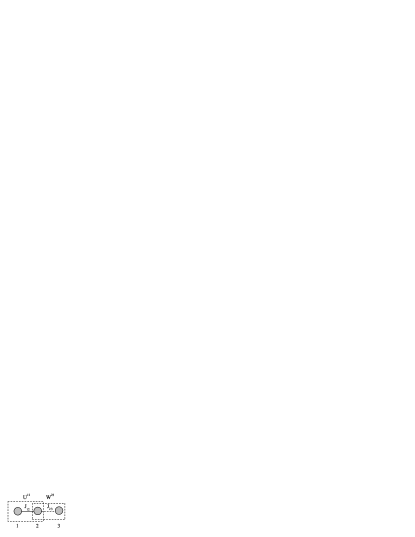
Figure 1: The spin chain including the target spin ($3$) used for implementing the IQST. The XY- interactions in the spin chain, denoted by the solid line, is always active, while the XY- interaction between spins $2$ and $3$, denoted by the dashed line, can be switched on and off. $W^{23}$ denotes the end gate applied to spins 2 and 3. $U^{12}$ denotes the evolution of spin chain.

We illustrate the IQST proposed in Ref. Bose using a system of three spins coupled by Heisenberg XY- interactions, as shown in Figure 1. The spin chain consists of spins $1$ and $2$, which are coupled by a constant (time-independent) interaction. Spin 3 is the target spin used to receive the transferred quantum state. The interaction between spins $2$ and $3$ can be switched on and off. Our purpose is to transfer an arbitrary quantum state $\alpha|0\rangle+\beta|1\rangle$ from spin $1$ to $3$, where $\alpha$ and $\beta$ are two complex numbers normalized to $|\alpha|^{2}+|\beta|^{2}=1$.

The Hamiltonian of the the spin chain without the end qubit is

$$H_{12}=\frac{1}{2}\pi J_{12}(\sigma_{x}^{1}\sigma_{x}^{2}+\sigma_{y}^{1}\sigma_{y}^{2}),$$ (1)

where $J_{12}$ denotes the coupling strength. The Hamiltonian of spins $2$ and $3$ is

$$H_{23}(t)=\frac{1}{2}\pi J_{23}(t)(\sigma_{x}^{2}\sigma_{x}^{3}+\sigma_{y}^{2}\sigma_{y}^{3}),$$ (2)

where $J_{23}(t)$ is $J_{23}$ when the interaction is switched on and $0$ otherwise.

II.2 IQST algorithm

The purpose of the IQST algorithm is the transfer of an arbitrary state $\alpha|0\rangle+\beta|1\rangle$ from the start of the chain (qubit 1) to the end (qubit 3). We start the discussion by choosing as the initial state of the complete 3-qubit system the state $\alpha|000\rangle+\beta|100\rangle$, i.e. a product state with spin $1$ in state $\alpha|0\rangle+\beta|1\rangle$, and spins $2$ and $3$ in $|0\rangle$. Transferring the $\alpha|0\rangle$ part of the input state is trivial, since spins 1 and 3 are in the same state and this state is invariant under the $XY$ interaction. We therefore only have to consider the $\beta|1\rangle$ part.

The chosen initial state of the spin chain is not unique. We could, e.g., choose to start with the total system in $\alpha|011\rangle+\beta|111\rangle$. In this case, the $|111\rangle$ is invariant and only the transfer of the $\alpha|0\rangle$ part needs to be considered. At the end of this section, we discuss additional possibilities.

The iterative transfer scheme of Burgarth et al. consists of a continuous evolution under the spin-chain Hamiltonian, interrupted by successive applications of the end-gate operation. We write the transfer operator as

$$T_{k}=\prod_{n=1}^{k}W^{23}(c_{n},d_{n})U^{12}(\tau)$$ (3)

where

$$U^{12}(\tau)=e^{-i\tau H_{12}}\otimes I^{3}=\left(\begin{array}[]{cccc}1&0&0&0\\ 0&C_{12}&-iS_{12}&0\\ 0&-iS_{12}&C_{12}&0\\ 0&0&0&1\end{array}\right)\otimes\left(\begin{array}[]{cc}1&0\\ 0&1\end{array}\right)$$ (4)

represents the evolution of the spin chain and

$$W^{23}(c_{n},d_{n})=\left(\begin{array}[]{cc}1&0\\ 0&1\end{array}\right)\otimes\left(\begin{array}[]{cccc}1&0&0&0\\ 0&d_{n}^{*}&c_{n}^{*}&0\\ 0&-c_{n}&d_{n}&0\\ 0&0&0&1\end{array}\right)$$ (5)

the end gate operation. Here, $C_{12}=\cos(\pi J_{12}\tau)$ and $S_{12}=\sin(\pi J_{12}\tau)$ and $n$ represents the iteration step. The parameters $c_{n},d_{n}$ are related by the unitarity condition $|c_{n}|^{2}+|d_{n}|^{2}=1$. For each step of the iteration, they are equal to the coefficients of the relevant states $|010\rangle$ and $|001\rangle$ just before the gate is applied. Under this condition,

$$W^{23}(c_{n},d_{n})(c_{n}|010\rangle+d_{n}|001\rangle)=|001\rangle,$$

i.e. the transfer to the final state $|001\rangle$ is maximized.

During the $n^{th}$ step, the two coefficients are

$$c_{n}=-i\frac{S_{12}C^{n-1}_{12}}{\sqrt{1-C_{12}^{2n}}},$$ (6)

$$d_{n}=\sqrt{\frac{1-C_{12}^{2(n-1)}}{1-C_{12}^{2n}}}.$$ (7)

II.3 Quantification of transfer

After $k$ iterations, $|100\rangle$ is transferred to

$$|\Psi_{k}\rangle=T_{k}|100\rangle=C_{12}^{k}|100\rangle+\sqrt{1-C_{12}^{2k}}|001\rangle.$$ (8)

Apparently, the transfer increases monotonically with the number of iterations and can asymptotically approach unity provided $|C_{12}|<1$. Writing $F_{k}=\langle 001|\Psi_{k}\rangle$ for the overlap of the system with the target state, we find

$$F_{k}=\sqrt{1-C_{12}^{2k}}.$$ (9)

Eq. (3) implies that only the spin chain or the end gate are active at a given time. If the spin chain interactions are static (not switchable), this can only be realized approximately if the coupling between the two end-gate qubits is much stronger than the couplings in the spin chain, $J_{23}\gg J_{12}$. In the NMR system, we instead refocus the spin-chain interaction during the application of the end-gate operation to better approximate the ideal operation

$$W^{23}(c_{n},d_{n})=e^{-i\pi J_{23}t_{n}(\sigma_{x}^{2}\sigma_{x}^{3}+\sigma_{y}^{2}\sigma_{y}^{3})/2}$$ (10)

where

$$\tan(\pi J_{23}t_{n})=-ic_{n}/d_{n}\,.$$ (11)

II.4 Generalization to mixed states

The IQST algorithm works also when the spin chain is in a suitable mixed state. As an example, we choose $\alpha=\beta=\frac{1}{\sqrt{2}}$. The second and third qubit can be chosen in any combination of $|0\rangle$ and $|1\rangle$. Here, we implement all four possibilities in parallel parallel by putting qubits 2 and 3 into the maximally mixed state $I^{2}\otimes I^{3}$, where $I$ denotes the unit operator and the upper index labels the qubit. The sample thus contains an equal number of molecules with qubits in the states $\alpha|0l\rangle+\beta|1l\rangle$ with $l=\{00,01,10,11\}$. The traceless part of the corresponding density operator is Chuang

$$\rho_{ini}=\sum_{l=00}^{11}\sigma_{x}^{1}\otimes(|l\rangle\langle l|).$$ (12)

If the system is initially in one of the states $|l\rangle=|01\rangle,|10\rangle$, it acquires an overall phase factor of $-1$ during the transfer. Combining this with the results of Sec. II.2, we find that after $k$ iterations, the system is in the state

$$\rho_{k}=T_{k}\,\rho_{ini}\,T_{k}^{{\dagger}}=\sqrt{1-F_{k}^{2}}\,\sigma^{1}_{x}\,I^{2}I^{3}+F_{k}\,\sigma^{1}_{z}\sigma^{2}_{z}\sigma^{3}_{x}.$$ (13)

Similarly, when the initial state is chosen as

$$\rho_{ini}=\sum_{l=00}^{11}\sigma_{y}^{1}\otimes(|l\rangle\langle l|),$$ (14)

the algorithm generates the state

$$\rho_{k}=T_{k}\rho_{ini}T_{k}^{{\dagger}}=\sqrt{1-F_{k}^{2}}\,\sigma^{1}_{y}I^{2}I^{3}+F_{k}\,\sigma^{1}_{z}\sigma^{2}_{z}\sigma^{3}_{y}$$ (15)

after $k$ iterations.

III Implementation

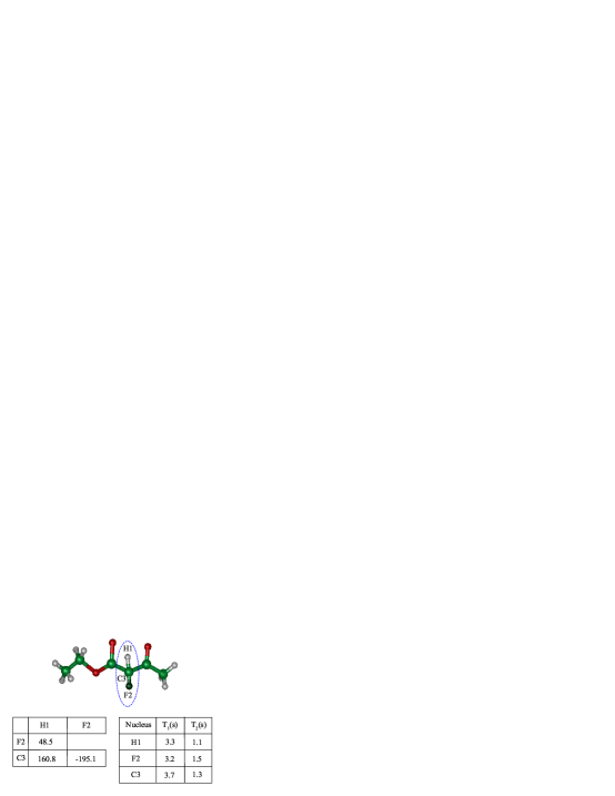
Figure 2: (Color online) The chemical structure of Ethyl 2-fluoroacetoacetate. The three spins in the dashed oval are the three qubits for implementing IQST. The strengths (in Hz) of the $J$-couplings between the relevant nuclear spins and the relaxation times are listed in the left and right tables, respectively.

For the experimental implementation, we chose the ¹H, ¹⁹F, and ¹³C spins of Ethyl 2-fluoroacetoacetate as qubits. The chemical structure of Ethyl 2-fluoroacetoacetate is shown in Figure 2, where the three qubits are denoted as H1, F2, and C3, respectively. The strengths of the $J$-couplings are $J_{12}=48.5$ Hz, $J_{23}=-195.1$ Hz and $J_{13}=160.8$ Hz. $T_{1}$ and $T_{2}$ values for these three nuclei are listed in the right table in Figure 2. In the rotating frame, the Hamiltonian of the three- qubit system is Chuang ; Ernst ; CoryPRL99

$$H_{NMR}=\frac{\pi}{2}(J_{12}\sigma^{1}_{z}\sigma^{2}_{z}+J_{23}\sigma^{2}_{z}\sigma^{3}_{z}+J_{13}\sigma^{1}_{z}\sigma^{3}_{z}).$$ (16)

The sample consisted of a 3:1 mixture of unlabeled Ethyl 2-fluoroacetoacetate and d6-acetone. Molecules with a ¹³C nucleus at position 2, which we used as the quantum register, were therefore present at a concentration of about $1\%$. They were selected against the background of molecules with ¹²C nuclei by measuring the ¹³C signal. We chose H1 as the input qubit and C3 as the target qubit. Figure 3 (a) shows the ¹³C NMR spectrum obtained by applying a readout pulse to the system in its thermal equilibrium state. Each of the resonance lines is associated with a specific spin state of qubits 1 and 2.

III.1 Initial state preparation

The initial pseudo-pure state $|000\rangle$ is prepared by spatial averaging spatial . The following radio-frequency (rf) and magnetic field gradient pulse sequence transforms the system from the equilibrium state

$$\rho_{eq}=\gamma_{1}\sigma_{z}^{1}+\gamma_{2}\sigma_{z}^{2}+\gamma_{3}\sigma_{z}^{3}$$ (17)

to $|000\rangle$: $[\phi_{1}]_{y}^{1}-[\phi_{2}]_{y}^{2}-[grad]_{z}-[\pi/2]^{1}_{x}-[1/2J_{13}]-[-\pi/2]^{1}_{y}-[\pi/4]^{3}_{x}-[-1/2J_{23}]-[-\pi/4]^{3}_{y}-[grad]_{z}-[\pi/4]^{1}_{x}-[1/2J_{13}]-[-\pi/4]^{1}_{y}-[grad]_{z}$. Here $\gamma_{1}$, $\gamma_{2}$ and $\gamma_{3}$ denote the gyromagnetic ratios of H1, F2, and C3, respectively, and $\cos\phi_{1}=2\gamma_{3}/\gamma_{1}$, and $\cos\phi_{2}=\gamma_{3}/2\gamma_{2}$. $[grad]_{z}$ denotes a gradient pulse along the $z$- axis. $[\pi/2]_{x}^{1}$ denotes a $\pi/2$ pulse along the $x$- axis acting on the H1 qubit. Overall phase factors have been ignored.

The coupled-spin evolution between two spins, for instance, $[1/2J_{13}]$, can be realized by the pulse sequence $1/4J_{13}-[\pi]^{2}_{y}-1/4J_{13}-[-\pi]^{2}_{y}$, where $1/4J_{13}$ denotes the evolution caused by $H_{NMR}$ for a time $1/4J_{13}$ ZZcouple .

The target state can be prepared directly from the state $|000\rangle$ by applying a $[\pi/2]^{3}_{y}$ pulse. It corresponds to $|00\rangle(|0\rangle-|1\rangle)/\sqrt{2}$, i.e. to transverse magnetization of the target spin, with the first two qubits in state $|00\rangle$. If we measure the free induction decay (FID) of this state and calculate the Fourier transform of the signal, we obtain the spectrum shown in Figure 3 (b). This spectrum serves as the reference to which we scale the data from the IQST experiment.

The input state for the IQST is $|\Psi_{in}\rangle=|\psi(\theta)\rangle|00\rangle$. We generate this state by rotating H1 by an angle $\theta$ around the $y$-axis: $|\Psi_{in}\rangle=e^{i\theta\sigma^{1}_{y}/2}|000\rangle$. After $k$ iterations of the IQST algorithm, $|\Psi_{in}\rangle$ is transferred to

$$T_{k}|\Psi_{in}\rangle=[(1-F_{k})\cos(\theta/2)|0\rangle-\sqrt{1-F_{k}^{2}}\sin(\theta/2)|1\rangle]|00\rangle+|00\rangle F_{k}|\psi(\theta)\rangle.$$ (18)

Here, we have used Eqs. (8-9) and assumed $C_{12}\geq 0$, without loss of generality. Hence the state transfer can be observed through measuring carbon spectra.

For the mixed input state, $\rho_{ini}$ [Eq. (14)] can be generated from $\rho_{eq}$ through the pulse sequence Tseng

$$[\frac{\pi}{2}]_{x}^{3}-[\frac{\pi}{2}]_{x}^{2}-[grad]_{z}-[\frac{\pi}{2}]_{x}^{1}.$$ (19)

III.2 Effective XY-interactions

The IQST algorithm requires XY interactions, while the natural Hamiltonian contains ZZ couplings. To convert the ZZ interactions into XY type, we decompose the evolution $e^{-i\varphi(\sigma_{x}^{k}\sigma_{x}^{l}+\sigma_{y}^{k}\sigma_{y}^{l})}$ into $e^{-i\varphi\sigma_{x}^{k}\sigma_{x}^{l}}e^{-i\varphi\sigma_{y}^{k}\sigma_{y}^{l}}$ cory07 using $[\sigma_{x}^{k}\sigma_{x}^{l},\sigma_{y}^{k}\sigma_{y}^{l}]=0$, where $\varphi$ denotes an arbitrary real number. These tranformations can be implemented by a combination of radio-frequency pulses and free evolutions under the $J$-couplings: DuPRA03 .

$$e^{-i\varphi\sigma_{x}^{k}\sigma_{x}^{l}}=e^{\pm i\pi\sigma_{y}^{k}/4}e^{\pm i\pi\sigma_{y}^{l}/4}e^{-i\varphi\sigma_{z}^{k}\sigma_{z}^{l}}e^{\mp i\pi\sigma_{y}^{k}/4}e^{\mp i\pi\sigma_{y}^{l}/4}$$ (20)

$$e^{-i\varphi\sigma_{y}^{k}\sigma_{y}^{l}}=e^{\pm i\pi\sigma_{x}^{k}/4}e^{\pm i\pi\sigma_{x}^{l}/4}e^{-i\varphi\sigma_{z}^{k}\sigma_{z}^{l}}e^{\mp i\pi\sigma_{x}^{k}/4}e^{\mp i\pi\sigma_{x}^{l}/4}\,.$$ (21)

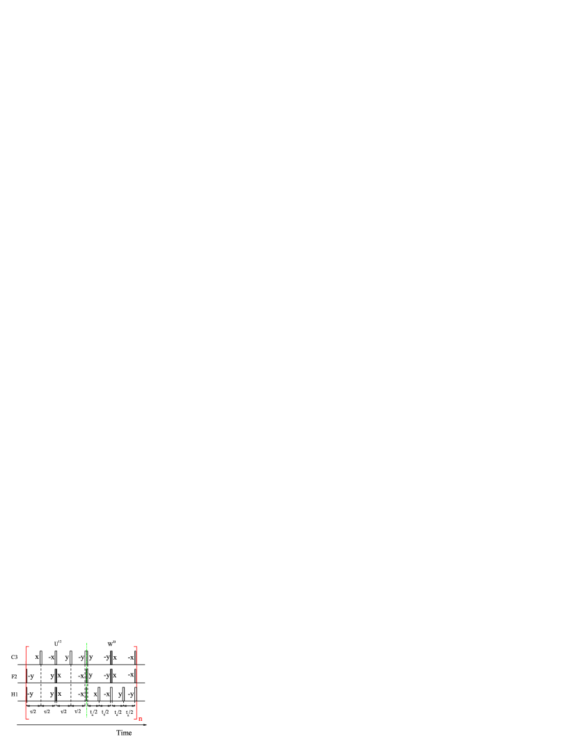
Figure 4: (Color online) Pulse sequence for implementing the IQST. The two blocks that implement $U^{12}(\tau)$ and $W^{23}(c_{n},d_{n})$ are separated by the dash-dotted line and ”$[...]_{n}$” indicates iteration $n$. The delays $t_{n}$ are given by Eq. (11). The narrow rectangles denote $\pi/2$ pulses, and the wide ones denote $\pi$ pulses, where $x$, $-x$, $y$, or $-y$ denote the direction along which the pulse is applied. The $\pi$ pulses are applied in pairs with opposite phases to reduce experimental errors Fang . The durations of the pulses are so short that they can be ignored.

Figure 4 shows the complete pulse sequence for implementing the IQST, starting from $|\Psi_{in}\rangle$. The subscript $n$ indicates that the pulses in the square brackets have to be repeated for every iteration. The duration of each $W^{23}$ segment varies, since $t_{n}=-\arctan(ic_{n}/d_{n})/\pi J_{23}$.

For the initial state $\rho_{ini}$ in Eq. (12), the propagators $n$ can be simplified: since the density operator commutes with $\sigma^{1}_{x}\sigma^{2}_{x}$ and $\sigma^{2}_{y}\sigma^{3}_{y}$ at all times, it is sufficient to generate the propagator

$$e^{-i\pi J_{23}t_{n}\sigma^{2}_{x}\sigma^{3}_{x}/2}e^{-i\pi J_{12}\tau\sigma^{1}_{y}\sigma^{2}_{y}/2}.$$

Similarly, for the initial state in Eq. (14), iteration $n$ can be replaced by $e^{-i\pi J_{23}t_{n}\sigma^{2}_{y}\sigma^{3}_{y}/2}e^{-i\pi J_{12}\tau\sigma^{1}_{x}\sigma^{2}_{x}/2}$. We use these simplified versions to shorten the duration of the experiment and thereby increase the fidelity.

III.3 Results for state transfer

When $\tau=1/2J_{12}$, the transfer can be implemented in a single step with a theoretical fidelity of $100\%$. The state transfer from H1 to C3 can be observed by measuring ¹³C spectra. The experimental result for $|\Psi_{in}\rangle=|\psi(\pi/4)\rangle|00\rangle$ is shown in Figure 5 (a). Comparing with Figure 3 (b) one finds that the output state is $|00\rangle(|0\rangle-|1\rangle)/\sqrt{2}$, i.e., the state $|\psi(\pi/4)\rangle$ is transferred from H1 to C3.

Figure 5 (b), show the corresponding result for the transfer of $\sigma_{y}^{1}$ from H1 to C3 in a single step, with qubits 2 and 3 initially in the completely mixed state. For this experiment, the receiver phase was shifted by $\pi/2$ with respect to the upper spectrum. Since this experiment implements the transfer for all possible states of the other qubits in parallel, we observe four resonance lines corresponding to the states $\{00,01,10,11\}$ of qubits 1 and 2. For the states with odd parity, the transfer adds an overall phase factor of -1, which is directly visible as a negative amplitude in the spectrum.

To demonstrate that iterative transfer works for a range of coupling strengths or (equivalently) evolution periods, we chose $\tau=1/5J_{12}$ and $\tau=1/6J_{12}$. For the case of pseudo-pure input states, three iterations are implemented for either case. When $\theta$ changes from $0$ to $2\pi$ the experimental results obtained from these transfer experiments are summarized in Figure 6, where the vertical axis denotes the amplitude of the NMR spectrum. For each input state the amplitude increases with the number of iterations. The increase of the amplitude shows the increase of the fidelity for the state transfer. The dependence on the input state parameter $\theta$ has the expected $\sin(\theta)$ dependence.

The experimental data obtained for the mixed input states are summarized in Figures 7 (a) and (b), for $\tau=1/5J_{12}$ and $\tau=1/6J_{12}$, respectively. The positive lines indicate that the transfer occurs with positive sign if qubits 1 and 2 are in state $|00\rangle$ or $|11\rangle$, and with negative sign for the states $|01\rangle$ or $|10\rangle$, in agreement with Eq. (15). Obviously the amplitude of the signals increases with the number of iterations. According to Eq. (15) the increase of the amplitudes is a direct measure for the progress of the quantum state transfer.

IV Discussion and Conclusion

Our results clearly demonstrate the validity of the iterative state transfer algorithm of Burgarth et al. In principle, it is possible to iterate the procedure indefinitely, always improving the fidelity of the transfer. In practice, every iteration also increases the amount of signal loss, either through decoherence or through experimental imperfections.

According to Eq. (15), the fidelity of the transfer is

$$F_{k}=|Tr[(\sigma^{1}_{z}\sigma^{2}_{z}\sigma^{3}_{y})\rho_{k}]|.$$ (22)

The experimental measurement corresponds to a summation of the amplitudes of the resonance lines. We normalized the experimental values to the amplitudes obtained by direct preparation of the target states [see Figure 3 (a)]. In Figure 8, we show the experimentally measured fidelities of the transfer of the state $\sigma_{y}$ for 1-5 iterations. As expected, the experimental data points are below the theoretical curves (full lines).

The experimental points can be fitted quite well if we include a decay parameter for each iteration. The dashed curves in Figure 8 represent the function $F_{k}e^{-kr}$ with $r=0.087$ and $r=0.079$ for $\tau=1/5J_{12}$ and $\tau=1/6J_{12}$, respectively. Each iteration thus adds imperfections (experimental plus decoherence) of about 8 %. Larger numbers of iterations are meaningful only if this error rate can be reduced.

In conclusion, we have implemented the iterative quantum state transfer in a three qubit NMR quantum information processor. The result shows that it is indeed possible to accumulate the quantum state at the end of a Heisenberg spin chain, whose couplings are always active.

V Acknowledgment

We thank Prof. Jiangfeng Du for helpful discussions. This work is supported by the Alexander von Humboldt Foundation, the DFG through Su 192/19-1, and the Graduiertenkolleg No. 726.

Figure 3: (a) ¹³C NMR spectrum obtained by applying a selective readout pulse to the system in its thermal equilibrium state. The four resonance lines correspond to specific states of the spin-chain qubits H1 and F2, as indicated by the labels above the resonance lines. The assignment takes into account that $J_{13}>0$ and $J_{23}<0$. (b) ¹³C NMR spectrum of the state $|00\rangle(|0\rangle-|1\rangle)/\sqrt{2}$, which was obtained by applying a $[\pi/2]_{y}^{3}$ pulse to $|000\rangle$.

Figure 5: Experimental results for quantum state transfer with $\tau=1/2J_{12}$. The initial states are $[|0\rangle-|1\rangle]|00\rangle/\sqrt{2}$ and $\sigma_{y}^{1}$, corresponding to figures (a) and (b), respectively. In the first experiment, the receiver phase was set to $x$, in the second experiment it was set to $y$.

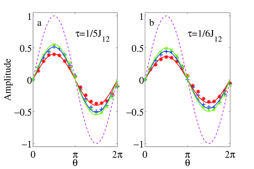
Figure 6: (Color online) Experimental results for demonstrating the IQST when the initial state is $[\cos(\theta/2)|0\rangle-\sin(\theta/2)|1\rangle]|00\rangle$. Two cases for $\tau=1/5J_{12}$ and $\tau=1/6J_{12}$ are shown in Figures (a) and (b). For each case three iterations are implemented. The experimental data after the completion of iteration 1, 2, and 3 are marked by ”*”, ”+”, and ”$\times$”, respectively. The data can be fitted as sin functions of which amplitudes represent the measured fidelities experimentally. The dashed curves show $\sin(\theta)$.

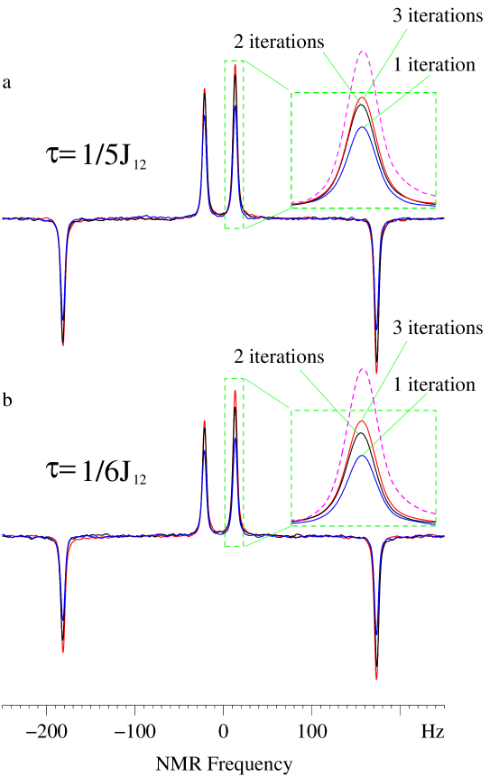
Figure 7: (Color online) ¹³C NMR spectra demonstrating the IQST of the state $\sigma_{y}^{1}$ for $\tau=1/5J_{12}$ and $\tau=1/6J_{12}$. For each case, the spectra after the completion of iteration 1, 2, and 3 are shown as the blue, black and red curves, respectively. The resonance lines corresponding to the $|00\rangle$ state of the spin chain are enlarged in the inset. The dashed curves are the corresponding sections of the reference spectrum in Figure 3 (a).

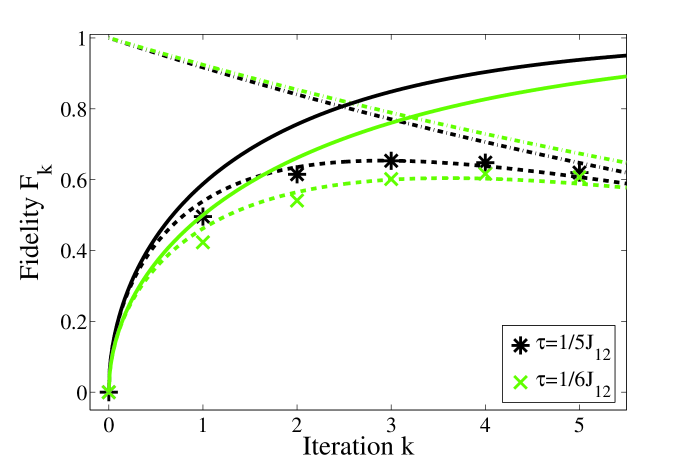
Figure 8: (Color online) Experimentally measured fidelity of the iterative state transfer as a function of the number of iteration steps when $\tau=1/5J_{12}$ and $\tau=1/6J_{12}$. The experimental data are fitted to the function $F_{k}e^{-kr}$ with $r=0.087$ and $0.079$ for the two cases, respectively. The two solid curves represent the theoretical fidelities $F_{k}$ for ideal conditions, and the two dash-dotted curves correspond to $e^{-kr}$. The dark and light curves correspond to the cases of $\tau=1/5J_{12}$ and $\tau=1/6J_{12}$, respectively.

References

• (1) M. A. Nielsen and I. L. Chuang, Quantum Computation and Quantum Information (Cambridge University Press, Cambridge, England, 2000); The Physics of Quantum Information, edited by D. Bouwmeester, A. Ekert, and A. Zeilinger (Springer, Berlin, 2000).
• (2) S. Bose, Phys. Rev. Lett. 91, 207901 (2003).
• (3) M. Christandl, N. Datta, A. Ekert, and A. J. Landahl, Phys. Rev. Lett. 92, 187902(2004); M. Christandl, N. Datta, T. C. Dorlas, A. Ekert, A. Kay, and A. J. Landahl, Phys. Rev. A 71, 032312(2005).
• (4) D. Burgarth, arXiv: 0704.1309 [quant-ph]; arXiv: 0706.0387 [quant-ph]; D. L. Feder, Phys. Rev. Lett. 97, 180502 (2006); A. Kay, ibid. 98, 010501 (2007); Phys. Rev. A 73, 032306 (2006); X.-F. Qian, Y. Li, Y. Li, Z. Song, and C. P. Sun, ibid. 72, 062329 (2005); P. Karbach and J. Stolze, ibid. 72, 030301(R) (2005); M.-H. Yung, ibid. 74, 030303(R) (2006); P. K. Gagnebin, S. R. Skinner, E. C. Behrman, and J. E. Steck, ibid. 75, 022310 (2007); V. Kostak, G. M. Nikolopoulos, and I. Jex, ibid. 75, 042319 (2007); O. Romero-Isart, K. Eckert, and A. Sanpera, ibid. 75, 050303(R) (2007); A. Bayat and V. Karimipour, ibid. 75, 022321 (2007); A. Wรณjcik, et al., ibid. 75, 022330 (2007); K. Eckert, O. Romero-Isart, and A. Sanpera, New J. Phys. 9, 155 (2007); P. Cappellaro, C. Ramanathan, D. G. Cory, arXiv:0706.0342 [quant-ph].
• (5) D. Burgarth, V. Giovannetti, S. Bose, Phys. Rev. A 75, 062327 (2007).
• (6) Z. L. Madi, R. Br$\ddot{u}$schweiler, and R. R. Ernst, J. Chem. Phys. 109, 10603 (1998).
• (7) C. H. Bennett, G. Brassard, C. Cr$\acute{e}$peau, R. Jozsa, A. Peres, and W. K. Wootters, Phys. Rev. Lett. 70, 1895 (1993); D. Boschi, S. Branca, F. D. Martini, L. Hardy, and S. Popescu, ibid. 80, 1121 (1998); D. Bouwmeester, J. Pan, K. Mattle, M. Eibl, H. Weinfurter, and A. Zeilinger, Nature (London) 390, 575 (1997); M. A. Nielsen, E. Knill, and R. Laflamme, ibid. 396, 52 (1998).
• (8) E. Knill and R. Laflamme, Phys. Rev. Lett. 81, 5672 (1998); A. Datta, S. T. Flammia, and C. M. Caves, Phys. Rev. A 72, 042316(2005); R. Stadelhofer, D. Suter, and W. Banzhaf, ibid. 71, 032345 (2005); G. L. Long, and L. Xiao, J. Chem. Phys. 119, 8473 (2003).
• (9) I. L. Chuang, N. Gershenfeld, M. G. Kubinec, and D. W. Leung, Proc. R. Soc. London, Ser. A 454, 447 (1998).
• (10) R. R. Ernst, G.Bodenhausen, and A.Wokaum, Principles of Nuclear Magnetic Resonance in One and Two Dimensions (Oxford University Press, Oxford, 1987).
• (11) S. Somaroo, C. H. Tseng, T. F. Havel, R. Laflamme, and D. G. Cory, Phys. Rev. Lett. 82, 5381 (1999).
• (12) D. G. Cory, M. D. Price, and T. F. Havel, Physica D 120, 82 (1998); J.-F. Zhang, G. L. Long, Z.-W. Deng, W.-Z. Liu, and Z.-H. Lu, Phys. Rev. A 70, 062322 (2004); X.-H. Peng, X.-W. Zhu, X.-M. Fang, M. Feng, X.-D. Yang, M.-L. Liu, and K.-L. Gao, arXiv:quant-ph/0202010.
• (13) L. M. K. Vandersypen, M. Steffen, M. H. Sherwood, C. S. Yannoni, G. Breyta, and I. L. Chuang, Appl. Phys. Lett. 76, 646 (2000); L. M. K. Vandersypen and I. L. Chuang Rev. Mod. Phys. 76, 1037 (2004); N. Linden, $\bar{E}$. Kup$\check{c}$e, and R. Freeman, Chem. Phys. Lett. 311, 321 (1999); X.-H. Peng, X.-W. Zhu, M. Fang, M.-L. Liu, and K.-L. Gao, Phys. Rev. A 65, 042315 (2002); R. Somma, G. Ortiz, J. E. Gubernatis, E. Knill, and R. Laflamme, ibid. 65, 042323 (2002).
• (14) C. H. Tseng, S. Somaroo, Y. Sharf, E. Knill, R. Laflamme, T. F. Havel, and D. G. Cory, Phys. Rev. A 61, 012302(1999).
• (15) J. S. Hodges, P. Cappellaro, T. F. Havel, R. Martinez, and D. G. Cory, Phys. Rev. A 75, 042320 (2007).
• (16) S. S. Somaroo, D. G. Cory and T. F. Havel, Phys. Lett. A 240, 1 (1998); M. D. Price, S. S. Somaroo, A. E. Dunlop, T. F. Havel, and D. G. Cory, Phys. Rev. A 60, 2777 (1999); J.-F. Du, H. Li, X.-D. Xu, M.-J. Shi, J.-H Wu, X.-Y Zhou, and R.-D. Han, ibid. 67, 042316 (2003); J.-F. Zhang, G. L. Long, W. Zhang, Z.-W. Deng, W.-Z. Liu, and Z.-H. Lu, ibid. 72, 012331 (2005); J.-F. Zhang, X.-H. Peng, D. Suter, ibid. 73, 062325 (2006).
• (17) X.-M. Fang, X.-W. Zhu, M. Feng, X.-A. Mao, and F. Du, Phys. Rev. A 61, 022307 (2000).
Refer to caption