Collisional processes and size distribution in spatially extended debris discs

Abstract

Context. New generations of instruments provide, or are about to provide, pan-chromatic images of debris discs and photometric measurements, that requires new generations of models, to in particular account for their collisional activity.

Aims. We present a new multi–annulus code for the study of collisionally evolving extended debris discs. We first wish to confirm and extend our early result obtained for a single–annulus system, namely that the size distribution in realistic debris discs always departs from the theoretical collisional “equilibrium” $\mathrm{d}N\propto R^{-3.5}\mathrm{d}R$ power law, especially in the crucial size range of observable particles ($R\la 1\,$cm), where it displays a characteristic wavy pattern. We also aim at studying how debris discs density distributions, scattered light luminosity profiles, and SEDs are affected by the coupled effect of collisions and radial mixing due to radiation pressure affected small grains.

Methods. The size distribution evolution is modeled over 10 orders of magnitude, going from $\mu$m-sized grains to $50$ km-sized bodies. The model takes into account the crucial influence of radiation pressure–affected small grains. We consider the collisional evolution of a fiducial, idealized $a$=$120$ AU radius disc with an initial surface density $\Sigma(a)\propto a^{\alpha}$. Several key parameters are explored: surface density profile, system’s dynamical excitation, total dust mass, collision outcome prescriptions.

Results. We show that the system’s radial extension plays a crucial role and that the waviness of the size distribution is amplified by inter–annuli interactions: in most regions the collisional and size evolution of the dust is imposed by small particles on eccentric or unbound orbits produced further inside the disc. Moreover, the spatial distribution of all grains $\la 1\,$cm significantly departs from the initial profile in $\Sigma(a)\propto a^{\alpha}$, while the bigger objects, containing most of the system’s mass, still follow the initial distribution. This has consequences on the scattered–light radial profiles which get significantly flatter, and we propose an empirical law to trace back the distribution of large unseen parent bodies from the observed profiles. We also show that the the waviness of the size distribution has a clear observable signature in the far-infrared and at (sub-)millimeter wavelengths. This suggests a test of our collision model, that requires observations with future facilities such as Herschel, SOFIA, SCUBA-2 and ALMA. We finally provide empirical formulae for the collisional size distribution and collision timescale that can be used for future debris disc modeling.

1 Introduction

Extrasolar discs around young stars have been imaged for more than two decades now. Observations and modeling have revealed the great diversity of these systems, in particular regarding the luminosity and density distribution of the dust component. Systems with the lowest dust to star luminosity ratios have been commonly labeled debris discs (e.g. Lagrange et al. 2000). The archetypal member of this group is $β$ Pictoris, which has been thoroughly observed and modeled since the first observation by Smith & Terrile (1984) (see reviews by Vidal-Madjar et al. 1994; Kalas & Jewitt 1995; Artymowicz 1997). These systems are believed to represent a later stage of disc evolution, where most of the initial solid mass has already been accumulated into planetary embryos or removed by collisional erosion and pressure forces (stellar radiation/wind pressure, see Greaves 2005; Meyer et al. 2006, for recent reviews on this subject). Simple order of magnitude estimates show that the dust in these systems cannot be primordial and has to be constantly replenished (Artymowicz 1997). Although cometary evaporation could also be a possibility (Li & Greenberg 1998), the most likely dust production mechanism is collisional erosion of bigger solid objects (Artymowicz 1997; Dominik & Decin 2003). This hypothesis is reinforced by the estimated ages of these systems, which are generally more than $10^{7}\,$yrs old (Greaves 2005). For such ages, the standard planetary formation model (e.g. Lissauer 1993) predicts that most early stages of planetary formation, i.e. grain coagulation, planetesimal formation, runaway and/or oligarchic accretion among these planetesimals, should already be over and that these systems should be made of large planetary embryos as well as smaller objects leftover from the formation process. The presence of big embryos should dynamically excite the system and lead to highly destructive mutual encounters between the smaller leftover bodies (Kenyon & Bromley 2004), thus triggering a collisional cascade producing objects down to very small dust grains.

The problems faced when modeling debris discs are numerous. One first difficulty is that all objects bigger than about $1\,$cm are completely undetectable by observations. Current observations only probe the lower tail of a collisional cascade among objects invisible to us. The challenge is thus to reconstruct this hidden bigger object population from the observed dust component. But even for particles in the “observable” range, it is very difficult to get a coherent global picture. Each type of observations (visible, near-IR, far-IR, mm,etc…) is indeed predominantly sensitive to one particle size range and to one radial region of the disc. And even when a large set of such observational data at different wavelengths is available (including spatially resolved images, as for example for $\beta$ Pictoris), it does not allow to straightforwardly reconstruct the dust population. This “connecting the dots” procedure is always model dependent because it depends on many parameters, linked to the dust’s composition, temperature, optical properties and size distribution, which can never be unambiguously constrained in a non–degenerated way (see for instance the thorough best–fit studies of Li & Greenberg (1998) and Augereau et al. (2001) for $\beta$ Pictoris or Su et al. (2005) for Vega). One challenge is in particular to get a coherent link between the mm–sized population, where most of the mass of the “dust” component is supposed to lie but for which spatial information is usually very poor, and the $\mu$m–sized grains, which should contain most of the optical depth and for which high–resolution observations are more and more frequently obtained.

2 Previous works and paper overview

The most basic way to perform these reconstructions of the unseen big objects population or to derive coherent models of the dust population is to assume that the classical collisional equilibrium size distribution of Dohnanyi (1969) in $\mathrm{d}N\propto R^{-3.5}\mathrm{d}R$ holds for all object sizes $R$. However, there are many reasons to believe that such an assumption is probably misleading. As it has been shown by Thébault et al. (2003, hereafter TAB03), the main problem arises from the smallest grains, whose behaviour is strongly affected by pressure forces imposed by the central star: radiation pressure in the case of luminous stars, wind pressure for low-mass stars (e.g. AU Mic, Augereau & Beust 2006; Strubbe & Chiang 2006). For stars of mass $M_{*}\ga 1\,M_{\odot}$, one major point is the presence of a minimum size cutoff $R_{\mathrm{PR}}$, all objects $R<R_{\mathrm{PR}}$ being blown away by radiation pressure. Qualitatively, this depletion of $R<R_{\mathrm{PR}}$ grains leads to an overdensity of slightly bigger grains $R_{1}$, because $R<R_{\mathrm{PR}}$ grains are depleted and can no longer efficiently destroy nor erode grains larger than $R_{\mathrm{PR}}$. The overabundance of $R_{1}$ grains, in turn, induces a depletion of $R_{2}$ objects with $R_{2}$ slightly larger than $R_{1}$, etc… This domino effect propagates towards bigger sizes and leaves a characteristic wavy size distribution, with a pronounced succession of overdensities and depletions with respect to the $R^{-3.5}$ power law (e.g. Campo Bagatin et al. 1994; Thébault et al. 2003; Krivov et al. 2006). These discrepancies with the $\mathrm{d}N\propto R^{-3.5}\mathrm{d}R$ distribution are reinforced by the fact that the smallest objects in the $R>R_{\mathrm{PR}}$ range are put on very eccentric orbits by radiation pressure and have a dynamical behaviour very different from that of the bigger non radiation-pressure-affected bodies (see Thébault et al. 2003, for a thorough discussion on this topic).

In TAB03 we quantitatively studied these complex effects for the specific case of the inner $β$ Pictoris disc. For this purpose, a statistical numerical code was developed, which quantitatively follows the size distribution evolution of a population of solid bodies, in a wide micron to kilometre size–range, taking into account the major effects induced by radiation pressure on the smallest grains (size cutoff, perturbed dynamical behaviour,…). Our main result was to identify an important departure from the $\mathrm{d}N\propto R^{-3.5}\mathrm{d}R$ law, especially in the $1\,\mu$m to $1$ cm range. The main limitation of this code is that it considers a single, isolated annulus. It can thus only be used to study a limited region at one given distance from the star ($\simeq 5\,$AU in the case considered) but not the system as a whole. A multi–annulus approach is needed to achieve this goal. Kenyon & Bromley (2002, 2004) have developed such statistical multi–annulus codes, which have been applied to various contexts. These codes are in some respect more sophisticated than the one used in TAB03, in particular because they follow the dynamical evolution of the system (which is fixed in TAB03). Nevertheless, the price to pay for following the dynamics is that the modeling of the small grain population is very simplified, with all bodies below a size $R\simeq\,1$ m following an imposed $R^{-q}\mathrm{d}R$ size distribution, thus implicitly overlooking the aforementioned consequences of the specific behaviour of the smallest dust particles. More recently, Krivov et al. (2006) used a different approach based on the kinetic method of statistical physics. This model is able to follow the evolution of both physical size and spatial distribution (1D) of a collisionally evolving idealized debris disc, from planetesimals down to $\mu$m–sized grains. This model has also the added advantage of taking into account a large range a unbound particles below the blow-out limit. This innovative approach gave promising results for the specific case of the Vega system. However, the modeling of collisional outcomes is, as acknowledged by the authors themselves, very simplified, with for instance all cratering impacts being neglected.

In this paper we present a newly developed multi–annulus version of our code, aimed at studying the collisional evolution of spatially extended systems. Intra and inter–annuli interactions, due to the radial excursions of radiation–pressure affected small grains, are considered. In addition to this new global scheme, a new and improved modeling of collision outcomes is presented, with particular attention paid to the crucial cratering regime (Section 3 and Appendix). In order to clearly identify and study the complex mechanisms at play, we consider in the present study the case of a fiducial idealized debris disc of $120$ AU radial extension, and explore surface density distributions in $\Sigma(a)\propto a^{\alpha}$ around the reference MMSN $\alpha=-1.5$ case, where $a$ is the distance to the star. The evolution of the system’s size distribution, and its significant departure from the standard Dohnanyi steady–state power law, is followed until $t=10^{7}\,$yrs and is presented in section 4. The role of several key free parameters, such as the system’s dynamical state, stellar mass and grain physical composition are explored in section 5. The evolution of the system’s spatial distribution, optical depth and the correspondence between observed dust and unseen bigger parent bodies is addressed in section 6. In section 7 we investigate the impact these results have on important observables, in particular the scattered light and thermal emission luminosity profiles as well as the SEDs. In section 8 we discuss the robustness of our results and derive empirical laws for the size distribution and collisional lifetimes which might be extrapolated to any kind of extended collisionally evolving debris disc. Conclusions and perspectives are presented in section 9. More specific studies of specific debris disc systems will be the purpose of a forthcoming paper.

3 Numerical model

3.1 Structure

Our code adopts the classical particle–in–a–box statistical approach to follow the collisional evolution of a population of solid bodies of sizes comprised between $R_{\mathrm{min}}\leq\,R_{\mathrm{PR}}$, where $R_{\mathrm{PR}}$ is the radiation pressure blow-out size, and $R_{\mathrm{max}}\simeq 10$–$50$ km. The system is made of $N_{a}$ concentric annuli of width $\Delta a_{ia}$ and centered at distances $a_{ia}$ from the star. Within each annulus $ia$, bodies are distributed into $n$ size bins, each bin corresponding to bodies of equal size $R_{i}$. The evolution of the size distribution with time is given by the estimated collision rates and outcomes between all collisionally interacting $(ia,i)$ bins. For small particles produced in an annulus $ia$ and placed on high-eccentricity or unbound orbits by radiation pressure, collisions with bodies located within all annuli crossed by their orbits are taken into account. A detailed presentation of the model is given in Appendix A.

One key parameter for our model, and any similar study for that matter, is the prescription for the collision outcomes. We adopt the classical approach where the outcome of an impact between a target of size $R_{t}$ and a projectile of size $R_{p}$ depends on the ratio between the center of mass specific kinetic energy of the colliding bodies $E_{\mathrm{col}}$ and the the so–called critical specific shattering energy $Q^{*}$, which depends on the objects’ sizes and composition. Depending on the respective values of these two parameters, impacts result in catastrophic fragmentation, cratering or accretion. The collision–outcome prescription has been updated with respect to the one in TAB03, in particular for what concerns the cratering regime. The new model now also accounts for differential chemical composition within the system, the main parameter being here the radial distance from the star $a_{\mathrm{ice}}$ below which water ice sublimates. The complete collision outcome procedure is described in more details in Appendix B. As explained in this Appendix, we consider a “nominal” case for the fragmentation and cratering prescriptions and with $a_{\mathrm{ice}}=20\,$AU, but other cases are explored (see section 5.4).

The price to pay for following the size distribution over more than 10 orders of magnitude in size is that we cannot accurately follow the dynamical evolution of the system, whose dynamical characteristics have to be fixed as inputs. In this case, all CPU–time consuming calculations of mutual impacting velocities and collision physical outcomes are performed once at the beginning of the run (e.g. TAB03, Krivov et al. 2006). We shall therefore implicitly assume that the disc has reached a quasi–steady dynamical state, which holds for timescales longer than the ones considered in the simulations. We consider identical average values for particle eccentricities and inclinations for all size bins, with the exception of bins corresponding to particles affected by radiation pressure for which specific orbital characteristics are numerically derived (see Appendix).

For a more detailed description of our code, see the Appendixies A and B.

3.2 Initial conditions

As mentioned in previous sections, we consider here a fiducial idealized debris disc, for which the initial spatial distribution follows the classical Minimum Mass Solar Nebulae (MMSN) profile derived by Hayashi (1981), where the surface number density is such that $\Sigma(a)\propto a^{-1.5}$, where $a$ is the distance from the star. We consider a $11$ concentric annulus disc, that extends from $a_{\mathrm{min}}=10$ AU to $a_{\mathrm{max}}=120$ AU, a typical range for the radial extension of dusty debris discs.

The initial conditions are chosen in accordance with the current understanding of debris discs, i.e. systems in which the bulk of planetesimal accretion process is already over and large planetary embryos are present. These large objects should dynamically excite the system, and average eccentricities and inclinations in the disc may reach values of the order of $0.1$ for Lunar–sized embryos (Artymowicz 1997). We thus take $\langle e\rangle=0.1=2\,\langle i\rangle$ (with $\langle i\rangle$ in radians) as our nominal dynamical conditions and explore different orbital values in separate runs. We follow the collisional evolution of all objects in the $[R_{\mathrm{min}},R_{\mathrm{max}}]$ range, where $R_{\mathrm{min}}\leq R_{\mathrm{PR}}$ and $R_{\mathrm{max}}\simeq 50\,$km. We take as a reference value $R_{\mathrm{PR}}=5\,\mu$m, which corresponds to the value for a compact grain around a $β$ Pictoris -like star (A5V), but other possible $R_{\mathrm{PR}}$ values for earlier and later type stars are also explored (section 5.2). The planetary embryos themselves are left out of our study since they are too isolated to contribute to the continuous collisional cascade, and can only affect the dust production rate through sudden isolated events (for the detailed study of such violent events, see Grigorieva et al. 2007). We shall assume that the initial size distribution at $t=0\,$yr follows the classical $\mathrm{d}N\propto R^{-3.5}\mathrm{d}R$ power law from $R_{\mathrm{min}}$ to $R_{\mathrm{max}}$ and we follow subsequent departures from this “equilibrium” distribution as time goes by. Having fixed the initial size–distribution, the initial disc mass is a free parameter which is explored in separate runs. This disc mass is parameterized by $M_{\mathrm{dust}}$, the total amount of ”dust”, i.e. grains smaller than $\simeq 1\,$cm, in the system. The parameter $M_{\mathrm{dust}}$ has been chosen as a reference because it is usually the most reliable constraint on the disc mass which can be derived from observations, since larger objects are observationally undetectable. Most of this dust mass is believed to be contained in the bigger millimetre–sized grains detected at sub–millimetre to millimetre wavelengths. Such millimetre wavelength surveys have shown that for debris discs around young main sequence stars, $M_{\mathrm{dust}}$ is typically comprised between $0.001$ and a few $0.1\,M_{\oplus}$ (e.g. review by Greaves 2005, and references therein). Accordingly, we shall consider two limiting cases: a low mass disc with $M_{\mathrm{dust}}=0.001M_{\oplus}$, and a high mass disc with $M_{\mathrm{dust}}=0.1M_{\oplus}$ (in both cases, the initial distribution of bigger objects is obtained by extrapolating a $\mathrm{d}N\propto R^{-3.5}\mathrm{d}R$ size distribution up to $R_{\mathrm{max}}$). Particles within the size bins are assumed to be compact silicates in the regions closer to the star than the subimation limit $a_{sub}$ and compact ices beyond $a_{sub}$, with $a_{sub}\simeq 20$AU in the nominal case (see section B.1 of the Appendix).

For each run, we let the system evolve for $10^{7}\,$yrs. Of course debris discs can have ages exceeding by far this value (as for instance Vega or $ϵ$ Eridani), and longer timescales should in principle be considered here. We should however restrict ourselves to $10^{7}$yrs because in most of the cases the system reaches a steady-state much earlier than this (typically after $\sim 10^{6}$years for our nominal case). The only exception to this is the “low–mass” case with $M_{\mathrm{dust}}=0.001M_{\oplus}$, for which the steady state is not reached, at $t_{\mathrm{final}}=10^{7}$yrs, in the outer regions of the systems. For this specific case, we let the system evolve until $10^{8}$yrs.

All initial parameters for the nominal high mass case are summarized in Table 1.

Table 1: Nominal case setup. The fields marked by a $\surd$ are explored as free parameters in the simulations. See text for details.

	Radial extension	$10<a<120\,$AU
	Number of annuli $\times$ radial width	$11\times 10$ AU
$\surd$	Initial surface density profile	$\Sigma(a)\propto a^{-1.5}$
$\surd$	Total “dust” mass ($R<1\,$cm)	$0.1\,M_{\oplus}$
	Size range modelled	$3\,\mu$m$<R<50$ km
	Number of size bins	$103$
	Initial size distribution	$\mathrm{d}N\propto R^{-3.5}\mathrm{d}R$
$\surd$	Sublimation distance (water ice)	$a_{\mathrm{sub}}=20\,$AU
$\surd$	Dynamical excitation	$\langle e\rangle=0.1=2\,\langle i\rangle$
$\surd$	Stellar type	A5V
$\surd$	Blow out size	$R_{\mathrm{PR}}=5\,\mu$m
$\surd$	Collision outcome prescription	(see Appendix B)

4 Results for the nominal case

4.1 High–mass disc ($M_{\mathrm{dust}}=0.1\,M_{\oplus}$)

Figure 1: High–mass case ($M_{\mathrm{dust}}=0.1M_{\oplus}$). Time-evolution of the size distribution at four different locations in the disc. Note that the $y$-axis displays the mass contained in one size bin, which is a correct way of displaying the mass distribution since all size bins are equally spaced in a logarithmic scale.

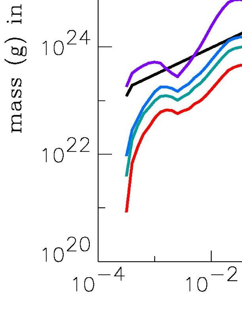
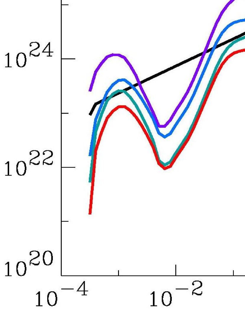
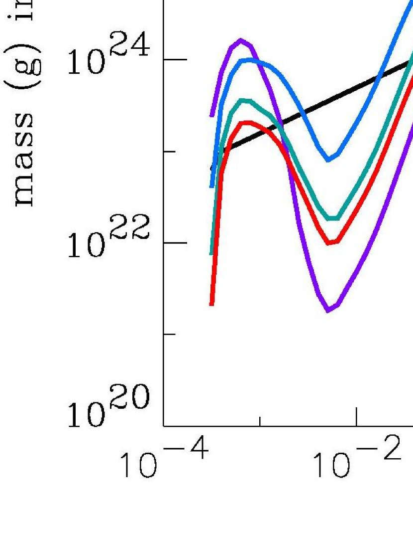
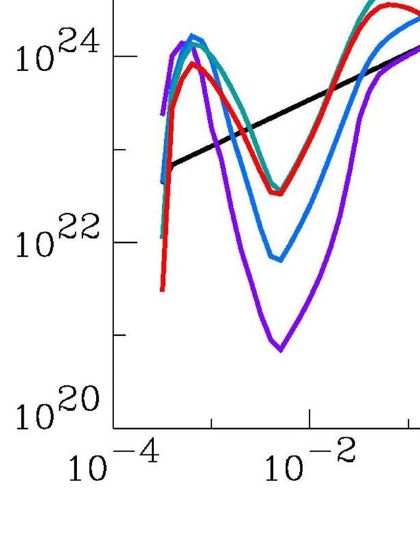
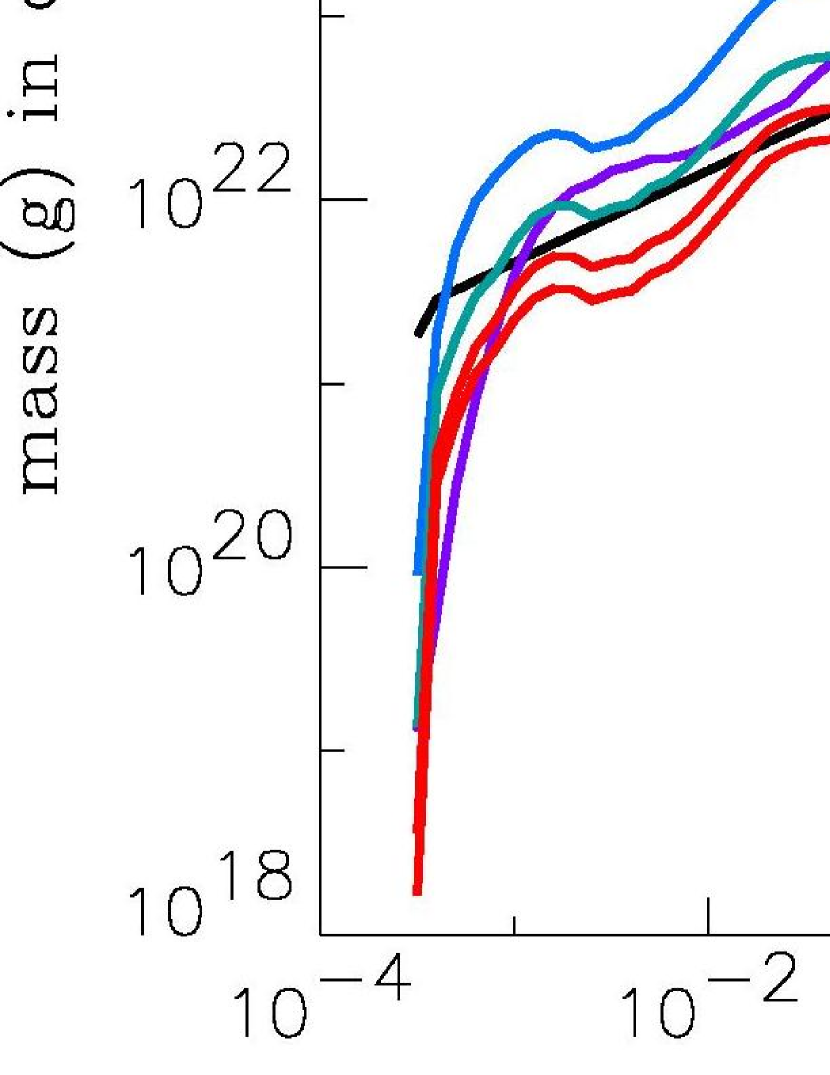
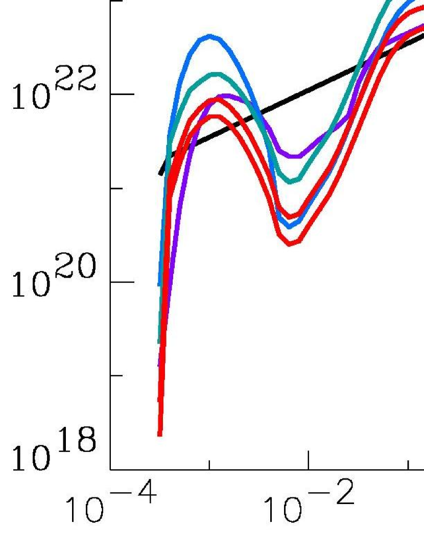
Figure 1 shows the evolution of the size distribution for four annuli at different distances from the star. In the innermost annulus (Fig. 1a), a weak wavy pattern develops, starting with the depletion of $R<R_{\mathrm{PR}}$ grains and propagating upward. Once the pattern has fully developed, subsequent evolution consists in a progressive total mass loss while the global size distribution profile is conserved. This wavy pattern is however much less pronounced in this innermost annulus than in TAB03. The first reason for this is that TAB03 considered a region further inside the disc, at $5$ AU, while the present inner annulus starts at $a=10\,$AU and extends up to $20\,$AU. Impact velocities, and their destructive efficiency, are thus significantly lower here. The second reason is due to our revised collision–outcome prescription, in particular for cratering events, which in TAB03 had a dominant role in shaping the size distribution in the $R\la 1\,$cm domain (see Table 4 of this paper). With the more realistic cratering prescription taken here, excavated masses are significantly smaller in the small grains domain than in TAB03 (see Sec. B.3), hence the shallower patterns in the size distribution. The knee in the distribution around $0.1$–$1$ km is a well known feature (e.g Campo Bagatin et al. 1994) due to the switch from the strength dominated regime, where bodies resistance weakly decreases with increasing size, to the gravity dominated regime, where bodies resistance to impacts rapidly increases with increasing size. It can be easily checked that the location of the knee at $R\simeq 0.1\,$km corresponds to the least impact–resistant bodies (see Equ. 12). Furthermore, for large objects, reaccumulation of fragments after an impact also begins to play a major role.

In the more distant annuli, on the contrary, very pronounced wavy patterns are observed in the size–distribution (Figs. 1b,c and d). The most striking features are the overdensity of $R\simeq 1.5\,R_{\mathrm{PR}}$ bodies, and above all, the strong depletion of bodies in the submillimetre range ($\simeq$ 10–50$\,R_{\mathrm{PR}}$). This result might appear counter–intuitive since one would expect these features to be even less pronounced than in the innermost annulus because of the longer dynamical timescales and lower impact velocities in the outer regions. The main cause for these sharp features are in fact small high–$\beta$ grains originating from other annuli further inside the disc (where $\beta$ classically designates the radiation pressure to gravitation forces ratio). This is clearly illustrated in Fig. 2 which compares, in the middle $50$–$60$ AU annulus, the final size distribution (solid line) with the size distribution obtained when only considering locally produced particles (dashed line). In the $R\la 30\,\mu$m range, foreign–born grains make up up to $90$% of the local population, thus resulting in a factor $\simeq 10$ increase of the number density. But the effect of these additional inner–disc–produced grains on the system’s evolution exceeds by far that simply due to a number density increase of an order of magnitude. Indeed, as these grains have had more time to reach high radial velocities than the locally produced grains of the same size, they will impact objects in the annulus at much higher relative velocities. As an example, for a target on a circular orbit at $50$ AU, an impact by a locally produced small grain with $\beta=0.45$, will occur at $\Delta v\simeq 1$ km.s^-1, whereas an impact by a $\beta=0.45$ grain produced at $10\,$AU will occur at $\Delta v\simeq 5\,$km.s^-1. This will result in much more destructive collisions. It is this higher destructive efficiency which is responsible for the deep depletion of objects up to $\simeq 100R_{PR}=0.5$ mm. Another important result is that a large fraction of the sub–mm grain depletion is due to cratering impacts, as appears clearly from the test run with no–cratering shown in Fig. 2 (dotted line). Indeed, small $R<30\,\mu$m grains cannot directly break–up objects bigger than $\simeq 0.1\,$mm, even for their increased impact velocities, while they can efficiently erode by cratering bodies up to almost $\simeq 1\,$cm.

Figure 2: Size distribution for the 50–60AU annulus, at $t=10^{7}\,$yrs, for the nominal case (solid line), when only taking into account fragmenting impacts, i.e. no cratering (dotted line), and when only taking into account the $locally$ produced grains, i.e. no impact with grains coming from inner annuli (dashed line)

4.2 Low–mass disc ($M_{\mathrm{dust}}=0.001\,M_{\oplus}$)

Figure 3: Evolution of the size distribution for the low–mass case ($M_{\mathrm{dust}}=0.001M_{\oplus}$).

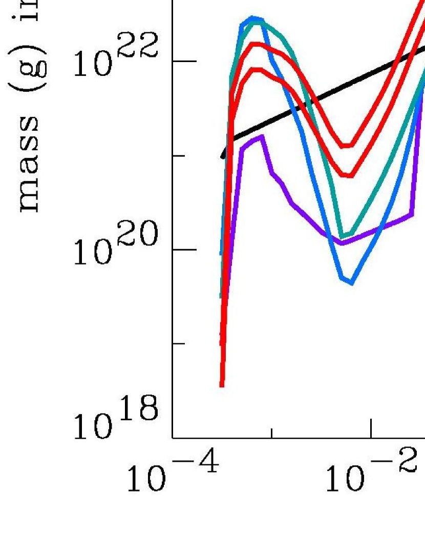
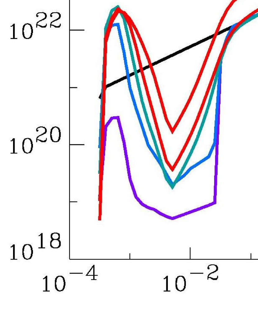
The evolution of the size distribution for the low-mass case is displayed in Figure 3. The main difference with the $M_{\mathrm{dust}}=0.1\,M_{\oplus}$ case is that the global evolution of the system is much slower. The slowing down is logically of the order of the discs mass ratio (i.e. a factor of about $100$). In the $a\la 70$ AU region, after $10^{7}\,$years, the system has reached a quasi steady–state relatively similar to the high mass case, with an overdensity of $\simeq 1.5\,R_{\mathrm{PR}}$ grains, followed by a depletion of sub–mm grains of approximately one order of magnitude compared to the initial size distribution.

In the outermost regions, however, we observe a much deeper depletion of sub–mm grains than in the high–mass case. This is because the collisional–equilibrium, contrary to the inner disc regions, has not been reached at $t=10^{7}$ years: the erosion of sub–mm grains, by high–$\beta$ particles coming from the inner regions, has already reached full efficiency (after less than $10^{4}\,$yrs), while the production of new sub–mm grains by erosion of larger objects occurs on much longer time–scales, exceeding $10^{7}\,$yrs in the outer regions (see more detailed discussion in the next section). This is clearly illustrated in Fig. 3d, which shows that, in the outermost annulus, the population of $>1$ cm objects remains largely unaffected by collisional processes after $10^{7}$ years. In order to get a better idea (and despite of the huge CPU-time cost), we decided to let this low-mass disc collisionally evolve for another $t=10^{8}$ years. As can be seen in Fig.3d, at this later time the quasi-steady state is almost reached in the outermost annulus, but the second “knee” in the size distribution at $R\simeq 0.1$km is still not visible yet. The full steady-state is here probably reached on timescales of the order of $\sim 1$ Gyr, which are presently out of the reach of our numerical code.

4.3 Collisional lifetimes

Figure 4: Collisional lifetimes of the particles as a function of their size, at $t=10^{7}\,$years, and at four different locations in the disc: $a=15\,$AU (solid line), $a=25\,$AU (dotted line), $a=55\,$AU (dashed line), $a=115\,$AU (dot-dashed line). The four horizontal lines are, for each distance, the collision timescales deduced from the simplified $T^{0}_{\mathrm{coll}}(a)=(\tau\Omega)^{-1}$ formula. The $a$ values refer to the center of the annulus where the particle has been produced. Left panel: high–mass case ($M_{\mathrm{dust}}=0.1M_{\oplus}$), right panel: low–mass case ($M_{\mathrm{dust}}=0.001M_{\oplus}$)

We define the collisional lifetime of a particle as the average time $t_{\mathrm{coll}}$ it takes for the object to lose $100\%$ of its mass by collisional processes. Let us point out that the collisional mass loss has two origins: (i) catastrophic fragmentation, for which a particle loses by definition $100\%$ of its mass at each fragmenting encounter, and (ii) cratering, for which the particle is progressively eroded after each impact (excavated mass $M_{\mathrm{cra}}$ given in App. B.3). The left and right panels of Fig. 4 display the values of $t_{\mathrm{coll}}(a,R)$, after $10^{7}$ years, at different radial locations in the disc, for both the nominal high–mass and the low–mass cases. Note that for particles placed on high–eccentricity orbits by radiation pressure, $t_{\mathrm{coll}}(a,R)$ is the collisional lifetime of a particle initially produced at distance $a$, when taking into account all the collisions this particle will suffer in the different annuli it will cross on its eccentric orbit.

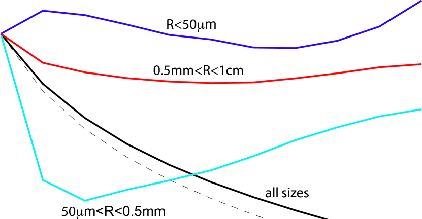
We discuss first the case of the high-mass disc (Fig. 4, left panel). For large objects, we obtain the predictable result that collision lifetimes increase with increasing distances from the star. This results from three concurring factors: particles number densities decrease with $a$, dynamical timescales get longer, and impact velocities lower, leading to less eroding impacts. For objects in the dust size range, however, the situation is much more complex, mainly because of the major influence the radial movements of small high–$\beta$ grains have on the collisional evolution. We find that the most short–lived particles are the ones with $R\simeq 100\,\mu$m, which logically corresponds to the most depleted population in the system (Fig. 1). For grains with sizes $R<100\,\mu$m, $t_{\mathrm{coll}}$ very rapidly increases with decreasing sizes. The explanation for this trend is twofold: first, destructive impactors in the $R<R_{\mathrm{PR}}$ range are strongly depleted, and second, many of these high–$\beta$ grains spend a large fraction of their eccentric orbits in the empty region of the disc beyond 120 AU. This global trend of the $t_{\mathrm{coll}}$ dependence with size could to some extent be compared to the one obtained by Strubbe & Chiang (2006) for the AU Mic system (where stellar wind from the central M-type star could play the same role as radiation pressure around A-type stars, see Augereau & Beust 2006). These authors also found $\mathrm{d}t_{\mathrm{coll}}/\mathrm{d}R>0$ for large grains and a very sharp $\mathrm{d}t_{\mathrm{coll}}/\mathrm{d}R<0$ gradient for smaller grains (see Fig.1 of this paper). However, these similarities are only qualitative (with major quantitative differences regarding the turn–off size or the slope of the $\mathrm{d}t_{\mathrm{coll}}/\mathrm{d}R$ laws) and should in any case be taken with great care, since the Strubbe & Chiang (2006) estimates were obtained for a radially narrow system and with a simplified analytical law for the collision rates and outcomes.

The relative lifetimes between different regions of the disc follow the logical trend in $\mathrm{d}t_{\mathrm{coll}}/\mathrm{d}a>0$, with the important exception of the innermost annulus, for which collisional lifetimes of small grains are relatively high, simply because there is here no flux of destructive small (high–$\beta$) impactors coming from further inside the system, contrary to the other annuli. Note that the only objects having $t_{\mathrm{coll}}>t_{\mathrm{final}}=10^{7}\,$yrs are the largest planetesimals, of size $R>0.2$ km in the outermost regions, and $R>3\,$km in the inner annuli. This means that, as a first approximation, all sub–kilometre sized objects are collisionally evolved, i.e., no object other than the largest kilometre–sized bodies are primordial.

All these global trends are also valid for the low–mass case (Fig. 4, right panel). However, the fraction of primordial objects is much higher than in the high–mass run. In the outer annulus, for example, no object bigger than $\simeq 1$ cm has been collisionally processed in $10^{7}$ yrs . This is in agreement with what was pointed–out in the previous section, namely that the collisional cascade did not fully develop in the outermost regions after $10$ Myr of evolution. For the dust–size range, however, the result that all particles are collisionally processed during the system’s lifetime still holds. This is why the shape of the size distribution is relatively similar in the high and low–mass runs.

As an interesting comparison, we also plotted on the graphs the collisional timescale obtained by the formula $t^{0}_{\mathrm{coll}}=(\tau\Omega)^{-1}$, where $\tau$ is the geometrical vertical optical depth and $\Omega$ the angular velocity. This simplified relation is indeed often used in the literature as giving an approximate estimate of the collision lifetimes of the smallest grains. As can be clearly seen, it proves to be a very poor match to our numerically derived lifetimes. Differences can reach up to 2 orders of magnitudes in the crucial $R<0.1$mm range.

5 Parameter dependence exploration

5.1 Dynamical excitation:   $\langle e\rangle$

Figure 5: Impact of the disc’s dynamical excitation on the size distribution after $10^{7}\,$years of evolution. The figure shows the size distribution of the whole system (i.e. all 11 annuli) assuming an initial dust disc mass of $M_{\mathrm{dust}}=0.1\,M_{\oplus}$ (high-mass case).

The exact orbital distribution of particles in debris discs is in general very poorly constrained. The only observational constraint comes from measuring the disc’s vertical thickness and deriving estimates of orbital inclinations, but such constraints are scarce. Edge-on discs represent the most favorable cases since $H/a$, where $H$ denotes the vertical scale height, can be directly measured. Five out of a dozen of spatially resolved discs have this particular orientation: $β$ Pictoris, AU Mic, HD 32297 (Schneider et al. 2005), HD 139664 (Kalas et al. 2006), HD 15115 (Kalas et al. 2007). For the two most studied discs, only partial information is available. Krist et al. (2005) find $H/a\la 0.04$ in the case of the AU Mic disc, with ratios as small as $0.02$ close to the position of maximum surface density. The $β$ Pictoris disc appears geometrically thicker with $H/a$ ratios as large as $\simeq 0.1$ (Golimowski et al. 2006). However, these measurements include the so-called disc warp which, according to Golimowski et al. (2006), might be due to a blend of two separate, intrinsically thinner disc components inclined with respect to each other by a few degrees. The $β$ Pictoris disc might then in fact be less vertically extended than it appears to be. The modeling and inversion of scattered light brightness profiles of inclined, ring-shaped discs do not provide much more constraints. The HR 4796 and HD 181327 rings for example, might have $H/a$ ratios as large as about $0.1$ at the positions of maximum surface density, but the actual ratios could be two times smaller (Augereau et al. 1999; Schneider et al. 2006). As pointed out in section 3.2, other estimates of the disc’s vertical thickness come from general theoretical arguments. Debris discs are indeed believed to correspond to the late stages of planetary formation where Lunar–to–Mars sized embryos dynamically excite the system. However, this argument can only lead to rough order of magnitude estimates of the dust’s orbital elements. It is thus important to explore different possible values of $\langle e\rangle$ and $\langle i\rangle$. Due to the CPU–time consuming aspect of the simulations, we chose to restrict ourselves to the high–mass system and perform one additional “dynamically colder” case with $\langle e\rangle=0.03=2\langle i\rangle$, one “very cold” system with $\langle e\rangle=0.01$ and one dynamically “hotter” case with $\langle e\rangle=0.2$. A comparison between these three cases and the nominal $\langle e\rangle=0.1$ case is displayed in Fig. 5. For sake of clarity, we consider here the whole system, summing up the contributions of all radial annuli.

Contrary to what could be intuitively expected, the depletion of objects smaller than $1\,$mm is more pronounced in the dynamically cold case $\langle e\rangle=0.03$ (Fig. 5). There are two concurring explanations for this apparent paradox. On the one hand, the rate at which sub–millimetre grains are eroded only weakly depends on the system’s dynamical excitation. Indeed, the velocity at which these grains are impacted by smaller micron–sized particles is mainly imposed by the strong radiation force acting on the latter and only weakly depends on the eccentricity of their parent bodies’ orbits. On the other hand, the rate at which big grains are produced, by impacts between larger objects, strongly depends on the system’s dynamical excitation, since these larger objects’ orbits, and thus their impact velocities, are insensitive to radiation pressure effects. As a consequence, the balance between production and erosion of sub–mm grains is more negative for low $\langle e\rangle$ values of the parent bodies orbits, hence the more pronounced depletion. For the “very” cold case, this effect is even more pronounced, and one can witness a global general depletion of $all$ dust size grains, while objects in the $\gtrsim 1$cm range are mostly unaffected by any collisional evolution.

Figure 6: Collisional lifetimes as a function of particle size, at $t=10^{7}\,$years for a dynamically “cold” case, $\langle e\rangle=0.03$ (left panel), and a dynamically “hot” case, $\langle e\rangle=0.2$ (right panel)

For the high–excitation case, the depletion of sub–mm grains is almost identical to the nominal case, which is here again a direct consequence of the fact that the dynamics of the very small grains is controlled by the radiation pressure force. These results are clearly illustrated in Fig. 6, showing the collisional lifetimes in both the dynamically “hot” and “cold” cases. While $t_{\mathrm{coll}}$ is roughtly inversely proportional to $\langle e\rangle$ for large ($\ga 1$cm) particles, the collisional lifetimes of small grains only weakly vary with the average dynamical excitation in the disc.

5.2 Mass of the star and $R_{\mathrm{PR}}$ value

The nominal case considered in our simulations is that of a $\beta$–Pictoris like star of mass $M_{*}=1.7\,M_{\odot}$ and a corresponding radiation pressure cut–off size $R_{\mathrm{PR}}=5\,\mu$m. We explore here the $M_{*}$ and $R_{\mathrm{PR}}$ parameters by considering, in addition to the nominal case, two limiting cases: one G–star of mass $1.1\,M_{\odot}$ with $R_{\mathrm{PR}}=1\,\mu$m, i.e., the lowest star mass for which compact silicate grains can reach the $\beta=0.5$ limit, and one Vega–like A0V star of mass $2.5\,M_{\odot}$ and $R_{\mathrm{PR}}=10\,\mu$m. All $R_{\mathrm{PR}}$ values have been derived using the Grigorieva et al. (2007) algorithm.

As appears clearly on Fig. 7, the size distributions for all three systems in the “dust” grains size range ($R<1\,$cm) are relatively similar. The profiles are shifted in size with respect to each other, reflecting the difference in $R_{\mathrm{PR}}$ values. Interestingly, the location of the overdensity of smallest grains is always given by the relation $R\simeq 1.5\,R_{\mathrm{PR}}$, while the most pronounced depletion is always obtained for $R\simeq 10-50\,R_{\mathrm{PR}}$. However, the amplitude of this depletion increases with increasing $R_{\mathrm{PR}}$ values (i.e. star masses). This is because, in the strength regime, smaller grains are more resistant to impacts than bigger ones, which implies that an impact between, say, a $R=1.5\,R_{\mathrm{PR}}$ dust grain and a $R=100\,R_{\mathrm{PR}}$ object is more erosive for larger values of $R_{\mathrm{PR}}$. Furthermore, for a more massive star, impact velocities are higher (for the same orbital parameters), which also leads to more destructive collisions.

Figure 7: Impact of the radiation pressure cut–off size value $R_{\mathrm{PR}}$ on the size distribution of the whole system (i.e. all 11 annuli) at $t=10^{7}\,$years for the high–mass case ($M_{\mathrm{dust}}=0.1\,M_{\oplus}$). Solid line: nomical case, $M_{*}=1.7\,M_{\odot}$ and $R_{\mathrm{PR}}=5\,\mu$m, dotted line:$M_{*}=1.1\,M_{\odot}$ and $R_{\mathrm{PR}}=1\,\mu$m, dashed line: $M_{*}=2.5\,M_{\odot}$ and $R_{\mathrm{PR}}=10\,\mu$m

5.3 Initial density profile

Figure 8: Size distribution, at $t=10^{7}\,$years, for the $whole$ system (all 11 annuli), for 4 different initial surface density distributions $\Sigma(a)\propto a^{\alpha}$, keeping the system’s total mass constant.

We have considered as a standard case a system following a standard MMSN spatial distribution in $\Sigma(a)\propto a^{-1.5}$. However, in order to check the robustness of our results, other indexes for the $\Sigma(a)\propto a^{\alpha}$ dependence have been explored. Fig. 8 shows that the global size distributions within the system only weakly depends on the initial $\Sigma(a)$ power law. The only noticeable trend is a slight damping of the wavy distribution in the $R\la$1cm range for flatter $\Sigma(a)$ profiles. This result is logical since we have seen in section 4.1 that, in a given region of the disc, the evolution of the sub–mm grains is mainly imposed by the flux of high–$\beta$ particles coming at high radial velocities from the inner regions. The influence of these inner–disc born grains should logically diminish for less steep $\Sigma(a)$ profiles, for which their relative abundance compared to the local population is smaller. However, these differences between the different $\Sigma(a)$ cases remain limited in amplitude and all size distributions remain very close to the result of the nominal case.

5.4 Collision outcome prescription

As discussed at length in the Appendix B, the collision outcome prescription is a poorly constrained parameter, first because of uncertainties regarding the chemical composition and structure of the grains and planetesimals in debris discs, and second because of significant differences between the predictions of all existing models. Our nominal case assumes a sublimation distance for ices $a_{\mathrm{sub}}=20\,$AU, the Benz & Asphaug (1999) prescription for the critical specific energy $Q^{*}$ for silicates and $Q^{*}_{\mathrm{ice}}=Q^{*}_{\mathrm{sil}}/5$, and the Koschny & Grün (2001) formula for crater–excavated masses $M_{\mathrm{cra}}$ for ices and silicates (see Appendix B). In order to explore how our results depend on the collision prescription, we have performed the two following additional runs:

• one “hard” material run, assuming the Benz & Asphaug (1999) and Koschny & Grün (2001) prescriptions for compact silicates hold for the entire disc (i.e. numerically setting $a_{\mathrm{sub}}=\infty\,$AU)

• One “weak” material run, where we assume the $Q^{*}$ prescription of Krivov et al. (2006), and a value of $M_{\mathrm{cra}}$ five times higher than in the nominal case.

The results are displayed in Fig. 9

As could be logically expected, the wave–like structure is much less pronounced for the “hard” material run. As a matter of fact, only the first wavy feature, affecting the smallest grains, is clearly visible, and its amplitude is damped by a factor $\simeq 3$ compared to the nominal case. Moreover, the size for which the strongest depletion is reached is shifted from $R\simeq 20R_{PR}=100\,\mu$m to $R\simeq 4R_{PR}=20\,\mu$m. For the “weak” material run, the exact opposite is observed: pronounced wavy–features propagate up to the largest sizes, and the amplitude of the depletion of sub–mm grains is significantly increased and reaches almost two orders of magnitude. Contrary to the hard–material run, the depletion is now shifted towards bigger grains as compared to the nominal run. The weak–material run partially resembles the results of Krivov et al. (2006), which is logical considering that we took identical $Q^{*}$ values, but differences are observed, which can probably be attributed to the fact that cratering impacts are here taken into account.

A comparison between Fig. 9 and all other parameter exploration runs of Figs. 5 to 8 clearly shows that the collision–outcome prescription is the most crucial parameter the final size–distribution depends on. Unfortunately, this parameter is probably the most poorly constrained in the present problem. As described at length in the Appendix, particular attention has been paid here to this crucial issue. We have tried to improve on most previous studies (including TAB03) and consider an upgraded model incorporating the most relevant available data for the $Q^{*}$ as well as fragmentation and, more specifically, cratering prescriptions. Nevertheless, large uncertainties remain. Firstly, important grain properties, which are crucial for understanding their response to impacts (ice fraction, porosity, etc…), remain poorly constrained for most debris discs. Secondly, even if all grain characteristics were fully known, it remains to see to which extent collision outcome energy–scaling models (even the more advanced version considered here), mostly obtained by experiments on cm–to–decimetre sized targets, might apply over such a wide size range, especially for very small micron–sized grains. There is to our knowledge no fully reliable data on what the outcome of a collision between, say, a 5$\mu$m grain and a 0.1mm target at 500m.s^-1 “really” is. Basically, it all comes down to how soft or hard (with respect to a collisional event) particles in the $<1$cm range are, and how these characteristics might vary with size. In this respect, we believe our nominal case collision prescription to be the most reliable one given the (still limited) current knowledge on this complex problem. Nevertheless, significantly different collisional behaviours cannot be ruled out. Fig. 9 probably gives a good idea of realistic boundaries for the limiting “hardest” and “weakest” material cases, showing that the waviness of the size distribution decreases with increasing collisional resistance of the objects.

Figure 9: Impact of the outcome collision prescription on the size distribution at $t=10^{7}\,$years and for the whole system (i.e. all 11 annuli). Three different collision-outcomes prescriptions have been assumed: nominal case (solid line), “hard material” case (dashed line) and “weak material” case (dotted line). See text for details.

6 Spatial distribution and dust to planetesimals mass ratios

6.1 Radial distribution

Figure 10: High–mass disc. Radial distribution, at $t=10^{7}\,$years, of the mass surface density for different object sizes. For each size range, all surface densities are renormalized to the surface density in the first annulus. The dashed line represents the theoretical distribution should a MMSN power law in $a^{-1.5}$ hold starting at the innermost annulus.

Figure 11: High–mass disc. Radial distribution, at $t=10^{7}\,$years, of the geometrical vertical optical depth for different size ranges, parametrized by their $\beta$ parameter.

For sake of clarity, we consider here only the nominal high–mass run. Fig.10 clearly shows that the spatial distribution significantly departs from the MMSN profile for all objects in the “dust” size range ($<1$cm). As could be logically expected, the strongest departure from the initial MMSN profile is obtained for grains in the sub-mm size range. For this population, the sharpest feature is a density drop in the regions just outside the first annulus. This drop is easily understandable and is due to the inter-annuli interactions already described in 3.1.1: in the innermost annulus, only $locally$ produced small grains can erode sub–mm particles, but such locally produced small grains, blown out by radiation pressure on unbound or very elliptical orbits, have not the time to be accelerated to high velocities, which limits their destructive or erosive power. In all other annuli, on the contrary, small grains coming from the inner regions impact local bigger grains at very high velocities and are able to deplete them more significantly.

For small grains in the $<50\,\mu$m range, the radial distribution is very flat, even flatter than the one which should be expected in a steady flow of outgoing unbound particles, where simple mass conservation considerations lead to $\Sigma(a)\propto a^{-1}$ (e.g. Su et al. 2005). This profile cannot be explained by simple blow out of unbound particles since most of the grains in the $<50\,\mu$m range are on $bound$ orbits ($R_{\mathrm{PR}}=5\,\mu$m for our nominal case). On the other hand, the mass surface density distribution of the total system (all particle sizes) is still relatively close to a classical MMSN profile in $a^{-1.5}$ (solid black line in Fig. 10). This is not an unexpected result, since the bulk of the disc’s mass is still contained in the biggest, kilometre–sized particles, which are only marginally affected by specific collisional behaviour of the smallest grains. Therefore, there exists a major discrepancy between the spatial distribution of the largest undetectable objects and that of the grains in the dust–size range, i.e. those accessible to observations.

Another interesting result concerns the geometrical vertical optical depth $\tau(a)$. Fig. 11 shows the respective weight of different grain populations. We see that, except for the innermost regions, $\tau(a)$ is completely dominated by grains from a very narrow size range of $\alpha$–meteoroids just above the blow–out limit $\beta=0.5\Leftrightarrow R=R_{\mathrm{PR}}$. Of course, even with a standard power law distribution in $\mathrm{d}N\propto R^{-3.5}\mathrm{d}R$, the optical depth should be dominated by small objects, since $\int\tau(R)\mathrm{d}R\propto\left(R^{-0.5}_{2}-R^{-0.5}_{1}\right)$. However, this tendency is much more pronounced here. As a matter of fact, when averaged over the whole system, it can be shown that 50% of the total optical depth is due to bodies in the $0.3<\beta<0.5\Leftrightarrow R_{\mathrm{PR}}<R<1.6R_{\mathrm{PR}}$ range. For a Dohnanyi profile, the size range containing 50% of the total optical depth is much broader: $R_{\mathrm{PR}}<R<4R_{\mathrm{PR}}$.

Figure 12: High–mass disc. Evolution of the vertical optical depth profile with time.

The temporal evolution of the $\tau(a)$ profile is also of interest. As Fig. 12 clearly shows, it rapidly settles (in a few $10^{5}$yrs) to a relatively “flat” radial profile, much flatter than the initial $a^{-1.5}$ one. This flattening is due to several mutually connected factors. The main one is due to what has been previously outlined, namely that the optical depth is dominated by grains from a narrow size range just above $R_{\mathrm{PR}}$. These very small grains are very quickly placed on very eccentric orbits, and will thus spend most of their orbits outside their annulus of production. As a consequence, small high-$\beta$ grains will naturally tend to be depleted in the inner regions and pile-up in the outer ones. In addition to this, the collisional erosion of bigger dust grains in the $\sim 0.05\,$mm to $1\,$mm range, which make up most of the mass “reservoir” from which smaller high-$\beta$ grains are collisionnaly produced, is faster in the inner regions than in the outer ones (see Fig. 1). For the innermost annulus, this significant mass erosion is even observed for the biggest planetesimals at the upper end of the size distributions (which get depleted by a factor $\sim 2$ in $10^{7}$yrs). It should be noted that the erosion of the $\sim 0.05\,$mm to $1\,$mm grains is sensitive to the collisional prescription: neglecting for instance cratering impacts leads to a much slower evolution of this population and thus a much slower flattening of the profile.

6.2 Link between dust and planetesimals

Table 2: Relative mass fraction $M_{\mu m}$ contained in the smallest ($R<20\,\mu$m) grains, $M_{mm}$ in the biggest dust particles ($0.1$ mm$<R<1\,$cm), and $M_{big}$ in the biggest $100\,$m$<R$ bodies, for all numerically tested cases and for a standard $\mathrm{d}N\propto R^{-3.5}\mathrm{d}R$ size distribution. All fractions are normalized to $M_{mm}$.

Run	$M_{\mu m}/M_{mm}$	$M_{big}/M_{mm}$
Nominal case	0.0678	3770.8
Low mass case	0.0744	1937.5
$\langle e\rangle$=0.01	0.0318	8515.7
$\langle e\rangle$=0.03	0.0278	3889.5
$\langle e\rangle$=0.2	0.1136	4476.2
Hard material case	0.0399	2137.7
Weak material case	0.0840	4112.3
$\Sigma(a)\propto a^{-0.5}$	0.0639	3655.3
$\Sigma(a)\propto a^{-1}$	0.0652	3634.2
$\Sigma(a)\propto a^{-2}$	0.0705	2958.1
$\mathrm{d}N\propto R^{-3.5}\mathrm{d}R$ distribution	0.0675	3510.8

As described at length in the introduction, an important issue is the link between the observed dust population and the unseen bigger parent bodies. We report in Table 2 the respective masses of 3 representative populations:

• the smallest $R<20\,\mu$m grains, i.e., the population containing most of the optical depth

• all grains in the $0.1\,$mm to $1$ cm range, i.e., where most of the observable “dust” mass is

• the biggest objects in the $R>100$ m range

Surprisingly enough, the respective masses between these 3 populations never drastically differ from their values in a standard Dohnanyi distribution. Both $M_{\mu m}/M_{mm}$ and $M_{big}/M_{mm}$ stay within a factor$\sim$3 above or below the reference values derived by integrating a $\mathrm{d}N\propto R^{-3.5}\mathrm{d}R$ power law. As a consequence, despite the strong wavy features of the size distributions, the link between the $total$ amount of observed dust and unseen bigger bodies can be, as a first approximation, derived using a simple Dohnanyi power law.

7 Impact on the observations

7.1 Scattered light surface brightness profiles

Figure 13: Synthetic luminosity profiles in scattered light (isotropic scattering), for the final states of all cases explored in section 5 (dashed lines); with the exception of those with alternative initial density profiles. All profiles have been renormalized to 1 at 10AU. The full line represents the theoretical brightness profile should a MMSN power law in $a^{-1.5}$ hold, for all grain sizes, starting at the innermost annulus. The dashed–dotted line represents the theoretical profile obtained when assuming a MMSN surface density in $a^{-1.5}$ for all bigger grains on Keplerian orbits, and assuming that all smaller radiation–pressure affected grains, up to $\beta<0.5$, are produced by the bigger grains following a size distribution in $R^{-3.5}$ (see text for details). Left panel: disc seen edge on, i.e., radial mid-plane profiles Right panel: disc seen head-on, i.e., average surface brightness.

7.1.1 Nominal case

We consider here the two limiting cases of edge–on and head–on viewed systems. For sake of simplicity, we have assumed gray scattering and we display results only for the pure isotropic scattering case. However, other scattering phase functions have been explored, and we verify that the results presented hereafter, in particular regarding the departure from the initial profiles, still hold for all explored cases. We furthermore assume the disc vertical scale height $H$ varies linearly with the distance to the star.

For the edge–on viewing case, Fig. 13 (left panel) shows that, surprisingly, the final mid–plane surface brightness (hereafter $S\!B$) profiles only weakly vary with the parameters explored in the different runs. For all 9 cases considered, the scattered light radial profiles approximately follow a power law in $S\!B_{\mathrm{edge}}(a)\propto a^{b}$ with $-2.4<b<-2.1$. This is very different from what is obtained for a theoretical system where all bodies follow the initial $\Sigma(a)\propto a^{\alpha}$ radial distribution and a Dohnanyi–like distribution holds over the whole size range, for which we get $b_{0}\simeq-3.4$ (for $\alpha=-1.5$), close to the theoretical value of $-3.5$ (e.g. Nakano 1990). We shall from now on refer to this theoretical disc, which in fact corresponds to the situation at $t=0$ in our simulations, as the “static” case, with $S\!B_{\mathrm{edge}}(a)\propto a^{b_{0}}$ and $b_{0}=\alpha-2$ (again assuming $H\propto a$). A similar result holds for the head–on case, for which average $S\!B$ profiles also strongly depart from the MMSN case (Fig. 13, right panel). In other words, $S\!B$ profiles cannot be simply derived by assuming the simplest hypothesis that dust grains follow the same spatial distribution as larger parent bodies (for which the initial $\Sigma(a)\propto a^{\alpha}$ profile still holds).

Interestingly, neither can these $S\!B$ profiles be derived by assuming the seemingly more advanced hypothesis that all small (i.e. radiation pressure affected) particles have eccentric orbits with their periastron coinciding with the big particles distribution and their number density being derived by the classical $\mathrm{d}N\propto R^{-3.5}\mathrm{d}R$ size distribution. This possibility has been checked following the method of Augereau et al. (2001) and Thébault & Augereau (2005): we run a simple deterministic orbital integration where $0<\beta<0.5$ grains are randomly produced from an initial parent body population (following here a surface density profile in $a^{-1.5}$). The distributions of all grains of a given $\beta$ are then obtained by phase mixing of their orbits and the total resulting surface density by weighting each contribution according to a Dohnanyi size distribution. The resulting mid–plane $S\!B$ profile is shown in Fig. 13 (triple dot-dashed line). Although it is a slight improvement over the pure “static” case, it is still far from all synthetic profiles obtained with our collisional evolution code. This means that the profile flattening is not simply due to the geometrical spread of high–$\beta$ grains on eccentric orbits. It is the consequence of the more complex effects these movements of radiation–pressure affected grains have on the collision production and destruction rates of dust grains in the different regions of the disc.

Figure 14: Normalized mid–plane surface brightness profiles in scattered light (isotropic scattering), for the 4 different initial density profiles explored in section 5. For each case, the full line represents the initial surface brightness profile, i.e. the profile obtained should the initial $\Sigma\propto a^{\alpha}$ distribution hold for all sizes, and the dashed line shows the final profile at $10^{7}\,$years.

Figure 15: Mean absorption cross section per unit of mass of material, $\kappa_{\lambda}$, at $t=10^{7}$ yr, for the nominal and low-mass cases (dashed and dotted line, resp.). The results are compared to the situation at $t=0\,$yr ($R^{-3.5}$ size distribution, solid green line), while the red triple-dot dashed line shows a power law fit to the long-wavelength part of $\kappa_{\lambda}$. The mean opacity obtained assuming the fit to the final size distribution (empirical formula given by Eq. 6) is overplotted (blue long-dashed line).

7.1.2 Comparison to observations

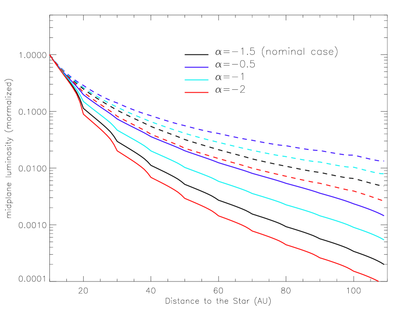
Different $S\!B$ profiles are obtained when starting from different initial radial distributions (cases explored in Sec. 5.3). However, we see that while $S\!B_{\mathrm{edge}}(a)$ profiles do vary with index $\alpha$, the differences between the initial and final profiles are remarkably similar, regardless of the initial $\Sigma(a)$ distribution. Fig. 14 shows indeed that, for all 4 explored initial $\Sigma(a)$ distributions, the initial $S\!B$ radial profiles always significantly flatten. The final profiles follow an approximate power law in $S\!B_{\mathrm{edge}}(a)\propto a^{b}$, whose index departs from the $t=0$ case by $\Delta b=b-b_{0}$, with $\Delta b$ comprised between $-1$ (for the $\Sigma(a)\propto a^{-0.5}$ distribution) and $-1.5$ ($\Sigma(a)\propto a^{-2}$ case). An even more interesting result is that, for a given system, these final surface brightness profiles $S\!B_{\mathrm{edge}}\propto a^{b}$ can be directly derived from the mass surface density distributions $\Sigma(a)\propto a^{\alpha}$ through the following relatively simple approximate empirical law:

$$S\!B_{\mathrm{edge}}(a)\propto a^{b}\,\,\leftrightarrow\,\,\Sigma(a)\propto a^{\alpha},{\rm\,\,\,\,with\,\,\,\,}\alpha=2b+3\,\,.$$ (1)

This relation, valid for isotropic scattering, slightly depends on the anisotropic scattering parameter $g$. Assuming a Henyey & Greenstein (1941) phase function, we find:

$$\alpha=2.4b+4.5 {\rm\,\,\,\,for\,\,\,\,} \mid g\mid=0.5$$ (2)

$$\alpha=3.3b+8.1 {\rm\,\,\,\,for\,\,\,\,} \mid g\mid=0.8\,\,.$$ (3)

A useful consequence of these relations is that they provide us with a tool to trace back the distribution of large parent bodies from the observed $S\!B$ profile. It is important to point out that the distribution of the small grains, those dominating the optical depth, can still be derived the “usual” way from the brightness profiles (using for example the $b=\alpha-2$ relation relation for constant opening discs and grey scattering). The important result is here that recontructing the optical depth distribution is not equivalent to reconstructing the mass reservoir distribution.

These results can usefully be compared to the radial luminosity profiles derived from observations. Although debris discs come in all sorts and shapes, the general tendency is that most of them have brightness profiles with a rather steep radial dependence in $S\!B\propto a^{b}$, with typically $-5<b<-3.5$ for edge-on discs or $-4<b<-3$ for head-on ones (e.g Ardila et al. 2004; Golimowski et al. 2006; Schneider et al. 2006; Kalas et al. 2006, 2007). These slopes are significantly steeper than the typical $S\!B_{edge}\propto a^{-2.2}$ obtained for our nominal case with large parent bodies following the MMSN radial distribution in $a^{-1.5}$. From our parameter exploration, only rather extreme cases would lead to edge-on brightness profiles in $\sim a^{-3.5}$. It would require either a very steep $\Sigma(a)\propto a^{-4}$ surface density profile (for the unseen parent bodies) or a very high, and probably unrealistic anisotropic scattering parameters ($\mid g\mid>0.9$). This apparent paradox between our simulation results, which we believe are rather robust with respect to the flattening of the optical depth and brightness profiles, and observations might be understood when recalling that our $S\!B_{edge}\propto a^{-2.2}$ profile is obtained within the regions where a complete collisional cascade is assumed to exist, from micron-sized grains all the way up to big planetesimals. There is no obvious reason why the full radial extents of observed debris discs should correspond to such collisionnaly active regions.

As a matter of fact, a large fraction of the luminosity radial profiles of spatially resolved discs could correspond to regions outside the “parent body” regions of collisional activity. For these regions outside the parent body area, preliminary analytical and numerical results seem indeed to show that a $a^{-3.5}$ slope could be a typical signature of the presence of high-$\beta$ grains escaping from their birth region (Strubbe & Chiang 2006; Krivov et al. 2006). This possibility is strengthen by the fact that for most debris discs, the steep slopes are derived in the outer regions located at relatively large distances from the star: beyond 120 AU for $β$ Pictoris  (Golimowski et al. 2006), 130 AU for HD 15115 (Ardila et al. 2004), $\sim 100\,$AU for HD 181327 (Schneider et al. 2006), $\sim 40$ AU for AU Mic (Krist et al. 2005), $55$ AU for HD 53143 (Kalas et al. 2006), $\sim 100$ AU for HD 32297 (Schneider et al. 2005). Within the frame of the “standard” planet formation scenario, it is likely that these regions are beyond the limit where accretion of large planetesimals/embryos is possible (e.g Thommes et al. 2003), so that the presence of collisional cascades starting from large parent bodies is questionable. As a consequence, our results imply (within the limitations to our approach outlined in section 8.3) that an observed $S\!B_{edge}\propto a^{-3.5}$ luminosity profile is the signature of either: 1) an extended parent body disc with a sharp $\Sigma\propto a^{-4}$ density decrease (Eq. 1) or, more likely, of 2) a region devoid of large particles beyond the main disc. One robust result is in any case that regions with steady collisional cascades from large parent bodies, probably cannot result in brightness profile signatures as steep as $S\!B_{edge}\propto a^{-3.5}$. Interestingly, for some systems where brightness profiles could be observationally derived in regions closer to the star, slopes closer to our nominal $b\sim-2.2$ value have been obtained. This is in particular true for $β$ Pictoris  where in the $\sim$70-100AU region where most of the dust mass is believed to reside, the brightness profile follows approximately $S\!B_{edge}\propto a^{-2}$ (Golimowski et al. 2006).

7.2 Thermal emission

7.2.1 Dust opacity

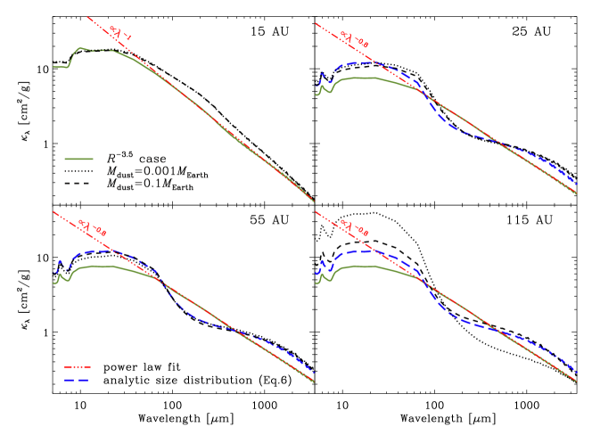
The waviness of the size distribution is well marked for grains smaller than a few centimetres radius, and should have an observational signature at far-IR, sub-mm and millimeter wavelengths. The four panels of Figure 15 show $\kappa_{\lambda}$, the absorption cross section per unit mass of solid material, averaged over the size distribution, at four different locations in the disc. The curves have been obtained assuming spherical grains made of a silicate core and coated by water ice beyond $20\,$AU (see Sec. B.1 for more details about the dust properties).

In the $\mathrm{d}N\propto R^{-3.5}\mathrm{d}R$ case, the mean opacity $\kappa^{0}_{\lambda}$ can be approximated by a power law $\kappa^{0}_{\lambda}\propto\lambda^{-q}$ beyond $\lambda\sim 70$–$100\,\mu$m, with $q\simeq 1$ for non-icy grains ($a\la a_{\mathrm{sub}}=20\,$AU), and $q\simeq 0.8$ beyond $a_{\mathrm{sub}}$. These $q$ values compare well with the theoretical estimates by Draine (2006), or the best fit values obtained for debris discs (e.g. Dent et al. 2000; Greaves et al. 2004). Nevertheless, Fig. 15 shows that realistic collisional systems do have mean opacities that strongly depart from a simple power law profile at long wavelengths. At representative distances from the star ($25$ AU and $55\,$AU), the mean opacity $\kappa_{\lambda}$ shows a characteristic dip at $\lambda\sim 150$–$200\,\mu$m, and a bump at millimetre wavelengths for both the nominal and low-mass cases. At $55\,$AU for example, the mean opacity ratio in the Spitzer/MIPS2 and MIPS3 bands, $\kappa_{70\,\mu\mathrm{m}}/\kappa_{160\,\mu\mathrm{m}}$, amounts to $1.7$–$2$ times the mean opacity ratio should a $R^{-3.5}\mathrm{d}R$ size distribution hold. Similarly, $\kappa_{520\,\mu\mathrm{m}}/\kappa_{160\,\mu\mathrm{m}}$, $\kappa_{850\,\mu\mathrm{m}}/\kappa_{160\,\mu\mathrm{m}}$, $\kappa_{1300\,\mu\mathrm{m}}/\kappa_{160\,\mu\mathrm{m}}$, are $1.7$, $2.1$ and $2.4$, respectively, larger than those found for a Dohnanyi size distribution.

In Sec. 8.1, we provide an anlytical fit to the final size distribution responsible for the waviness of the mean opacity. The mean opacity obtained assuming the empirical differential size distribution given by Eq. 6, compares well to that calculated at our representative distance of $55$ AU.

7.2.2 Disc SED and images

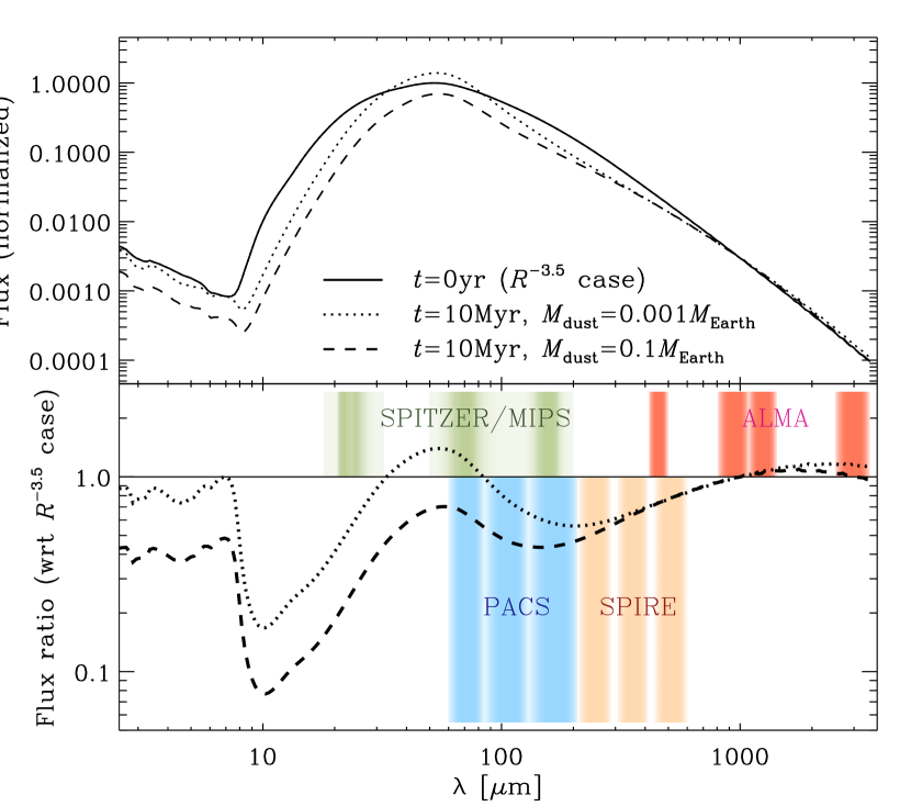
The actual impact on the disc spectral energy distribution (SED) is displayed in the top panel of Fig. 16, where the synthetic SEDs have been calculated using the model of Augereau et al. (1999). The solid line on the figure represents the disc SED, normalized to $1$ at its maximum, at $t=0$ ($\mathrm{d}N\propto R^{-3.5}\mathrm{d}R$ size distribution), and the bottom panel shows the flux ratio after $10\,$Myr of evolution of the system. As anticipated, the wavy structure of the size distribution has an observational counterpart at far-IR to millimetre wavelengths, and in particular a lack of emission in the $150$–$200\,\mu$m spectral range compared to the $R^{-3.5}$ size distribution. The predicted disc colors depart from the Dohanyi case by factors that compare to the mean opacity ratios calculated above. More precisely, the $70\,\mu$m to $160\,\mu$m, $520\,\mu$m to $160\,\mu$m, $850\,\mu$m to $160\,\mu$m, and $1300\,\mu$m to $160\,\mu$m flux ratios, are $1.5$–$2.1$, $1.3$–$1.8$, $1.6$–$2.2$ and $1.9$–$2.4$, respectively, larger than those found for a Dohnanyi size distribution.

The $150$–$200\,\mu$m spectral range clearly appears as a critical spectral range to test the model developped in this paper. It requires a good sampling of the SED at long wavelengths, and a sufficiently precise relative photometric calibration. Several observational facilities working at far-IR to millimeter wavelengths, will start operation in a very near future. Some of them are indicated in the bottom panel of Fig. 16, to which should be added the SCUBA-2 camera at JCMT (Holland et al. 2006), and the SOFIA observatory (Becklin 2006; Casey 2006). The PACS and SPIRE instruments onboard the Herschel space observatory are particularly well suited to identify the dip at around $150$–$200\,\mu$m by measuring the exact shape of debris discs SEDs beyond $\lambda\sim 70\,\mu$m (Pilbratt 2005; Poglitsch et al. 2006). This would allow to find a direct observational signature of an ongoing collisional cascade in a debris disc.

Figure 16: Disc SEDs, including both thermal emission and scattered light (which dominated over thermal emission at $\lambda\la 10\,\mu$m).

Figure 17: Appearance of the high–mass disc, assumed face-on, at $t=10\,$Myr as a function of the observing wavelength. Top panel: logarithmic scale. Bottom panel: linear scale.

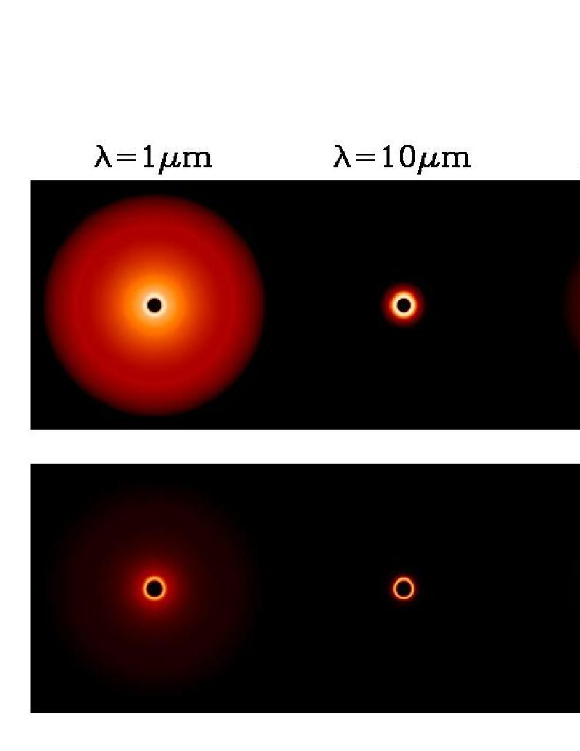
The dependence of the size distribution on the distance to the star, evidenced in Figs. 10 and 11, has direct consequences on the appearance of the disc, as illustrated in Fig. 17. In the near-infrared, and at shorter wavelengths, light scattering by small (high–$\beta$) particles dominates the disc image. The disc therefore shows a decreasing brightness profile with increasing $a$ as discussed in Sec. 7.1. In the thermal emission-dominated regim (mid-infrared and beyond), the disc morphology totally depends on the observing wavelength. At $\lambda=24\,\mu$m for instance, the disc surface brightness smoothly decreases with the distance from the star, while at (sub-)mm wavelengths, the disc shapes a ring peaked close to the outer edge of the parent-body disc ($\sim 100\,$AU), a situation that interestingly recalls the case of the Vega disc (Su et al. 2005).

8 Empirical formulae for debris disc modeling

The purpose of the present work is to numerically explore the collisional evolution of an extended debris disc, when taking into account the crucial effects of impacts induced by the radiation–pressure affected small grains. The different results displayed in Secs. 5 and 7 show that, although noticeable differences might be observed for different setups, important generic trends can be derived. We propose, in the following, empirical laws for the size distribution and collision timescales, that can be used for debris disc modeling as alternatives to the classical $R^{-3.5}$ size distribution and to the $t^{0}_{\mathrm{coll}}=\left(\tau\Omega\right)^{-1}$ law.

8.1 Fit to the size distribution

Figure 18: Dashed lines: Final size distribution profiles, averaged over the whole system, for all numerically tested cases, except the 2 “weak” and “hard” material cases with different collisional prescriptions. All profiles’ $x$–axis have been renormalized to units of $R_{\mathrm{PR}}$, and all $y$–axis to the value of the first wavy “peak” at $R\simeq 1.5R_{\mathrm{PR}}$. Solid line: reference profile derived from our empirical fit given by Equ. 4 and integrated over one logarithmic size interval: $\Delta M(R)=G(R)\left(R/1.5R_{\mathrm{PR}}\right)^{0.41}\Delta M_{(1.5R_{\mathrm{PR}})}$.

One crucial result concerns the final size distributions. For almost all runs, the system always quickly reaches a quasi steady–state, with a pronounced wavy distribution which strongly departs from a standard “equilibrium” distribution in $\mathrm{d}N\propto R^{-3.5}\mathrm{d}R$, or any simple power law in $R^{q}\mathrm{d}R$ for that matter. As clearly appears in Figs. 1 & 3, the waviness varies with location in the system, it is less pronounced close to the inner edge, since it is mostly due to collisions due to high velocity outward moving small grains. However, if ones considers the average distribution integrated over the whole disc, we have seen that its profile only weakly depends on parameters such as the system’s total mass, it’s dynamical excitation or the value of the radiation pressure cut–off size $R_{\mathrm{PR}}$. For the latter case, what is observed is mostly an offset of the wavy–distribution, which retains its global shape and main characteristics. As for the total initial mass, it does not crucially affects the final $shape$ of the size distribution as long as collision lifetimes of dust grains are shorter than the system’s age (see Sec. 4.2). The final size distribution is even relatively unaffected by the profile of the initial mass distribution (exponent of the $\Sigma(a)$ profile). The only cases for which a major modification of the size distribution is observed are the “very weak” and the “very hard” material cases. Apart from these 2 exceptions, for all other 10 tested setups we obtain very similar features: a strong depletion of $R\la R_{\mathrm{PR}}$ grains, a peak for $R\simeq 1.5R_{\mathrm{PR}}$ followed by a deep depletion of objects in the $10R_{\mathrm{PR}}<R\la 50R_{\mathrm{PR}}$ range. The similarities between all profiles are even more striking when they are renormalized by their value at $R=R_{\mathrm{PR}}$ (Fig. 18). As can be clearly seen, variations are very limited for $R\la 100R_{\mathrm{PR}}$. For this size range it seems thus reasonable to consider that, as a first approximation, the size distribution obtained in our nominal case is a relatively good standard for spatially extended systems. We were able to derive an empirical fit for this revised size distribution, valid in the $R\la 100R_{\mathrm{PR}}$ range. When written in terms of the differential mass distribution, it reads:

$$\mathrm{d}M\propto\,G(R)R^{-0.59}\mathrm{d}R$$ (4)

with

$$\log_{10}{\left(G(R)\right)}=\frac{2}{3}\left[\cos\left(2\pi\left[\left|\frac{1}{2}\log_{10}\left(\frac{R}{1.5R_{\mathrm{PR}}}\right)\right|\right]^{0.85}\right)-1\right]\,.$$ (5)

This new relation proves to be a reasonably good fit to almost all profiles in the $R\la 100R_{\mathrm{PR}}$ range (Fig. 18). In terms of the differential size distribution $\mathrm{d}N(R)$, this translates into

$$\mathrm{d}N\propto\,G(R)R^{-3.59}\mathrm{d}R\,,\,\,\mathrm{for}\,\,\frac{2}{3}R_{\mathrm{PR}}<R\la 100\,R_{\mathrm{PR}}\,.$$ (6)

Beyond $100\,R_{\mathrm{PR}}$, stronger divergences between different runs are observed. However, as a rough first order approximation, the differential size distribution can approximately be extrapolated by a $R^{-3.7}$ power law. The $R^{-3.7}$ extrapolation has been used to calculate the mean opacity represented by a blue long-dashed line in Fig. 15.

8.2 Fit to the collisional particle lifetime

Figure 19: Dashed lines: Collisional lifetimes at $a_{0}=55$AU, for all tested cases except the weak and hard material runs, when renormalized by the reference timescale $t_{\mathrm{coll-ref}}=t^{0}_{\mathrm{coll}}(a_{0})\left(\Omega(a_{0})\tau(a_{0})\right)^{-1}$. Solid line: profile derived from our empirical fit (Equs. 7 and 8)

As shown in Sec. 4.3, collisional lifetimes strongly vary with particle sizes: they increase very rapidly when $R$ gets close to the blow–out limit $R_{\mathrm{PR}}$, reach a sharp minimum around $R\simeq 10R_{\mathrm{PR}}$, increase sharply again between $10R_{\mathrm{PR}}$ and about $100R_{\mathrm{PR}}$ and then continue to increase much more slowly with increasing sizes (see Fig.4). We have also shown that a direct consequence of this result is that collisional lifetimes cannot be directly derived from the optical depth through the simplified formula $t^{0}_{\mathrm{coll}}(a)=(\tau\Omega)^{-1}$. There are several reasons why this formula cannot hold here:

• the $t^{0}_{\mathrm{coll}}(a)=(\tau\Omega)^{-1}$ formula implicitly considers impacts between objects of equal sizes, thus neglecting the broad size spectra of all possible impactors on a given target,

• it also implicitly assumes that all impacts are fully destructive, i.e., that the collision timescale is equal to the collisional lifetime. This neglects all cratering impacts, whose role is crucial for the considered problem (see Fig.2),

• even more important: this formula neglects all effects due to the specific dynamics of the smallest grains affected by radiation pressure,

• last but not least: at any given distance $a_{0}$ from the star, it neglects all collisions due to objects coming the inner $a<a_{0}$ regions, and it has been shown (Fig.2) that these collisions are crucial for the evolution of dust grains.

As can be seen for example in Figs. 4a,b and 6a,b, collisional timescales significantly vary for different initial conditions, in particular total initial mass and dynamical excitation of the system. However, the profiles of the $t_{\mathrm{coll}}(a,R)$ curves are relatively similar. In order to visualize these similarities more clearly, all $t_{\mathrm{coll}}(a,R)$ curves have been renormalized by the reference timescale $t^{0}_{\mathrm{coll}}(a)=(\tau\Omega)^{-1}$ (Fig.19). In a similar fashion as for the size distributions, we see that all normalized $t_{\mathrm{coll}}(a,R)$ profiles remain relatively close to the nominal case. This opens the possibility for deriving an empirical fit to $t_{\mathrm{coll}}(a,R)$ as a function of $a$ and $\tau$:

$$t_{\mathrm{coll}}(a,R)=t^{0}_{\mathrm{coll}}(a)\,\left[\left(\frac{R}{R_{1}}\right)^{-2}+\left(\frac{R}{R_{2}}\right)^{2.7}\right]\,\,\,{\rm for}\,\,\,R<R_{2}$$ (7)

with $R_{1}=1.2R_{\mathrm{PR}}$ and $R_{2}=100R_{\mathrm{PR}}$, and

$$t_{\mathrm{coll}}(a,R)=t^{0}_{\mathrm{coll}}(a)\,\left(\frac{R}{R_{2}}\right)^{0.3}\,\,\,\,\,\,\,\,\,{\rm for}\,\,\,R>R_{2}\,\,.$$ (8)

8.3 Approximations and limitations

Let us state again that these relations should be taken with care. An important general remark is to again stress that they have been derived for extended collisionally active regions, i.e., regions with steady collisional cascades starting from large reservoirs of big unseen parent bodies. These regions might not account for all the observed radial extent of debris discs: some observed regions are probably collisionally inactive areas where only small high-$\beta$ grains, produced in parent body regions further inside, are present (see discussion in Sec. 7.1.2).

Moreover, within the frame of our numerical approach it is important to point that these fits are valid for our nominal collision outcome prescription, and that significant variations should be expected for harder or weaker material prescriptions (Fig. 9). It should also be noted that in a “real” disc, all individual particles are not completely identical: they would have slightly different material compositions, porosities, differ in presence or absence of microcracks, etc… This might alter the size distribution profile, probably damping the waviness described in Eq. 6 to some extent, but such sophisticated effects are difficult to take into account with a particle-in-a-box code. Another important point is the fact that the smallest particles considered here are just below $R_{\mathrm{PR}}$, so that only 2 size “bins” correspond to unbound so-called “$\beta$-meteoroids”. We nevertheless performed a few test runs with additional small-size bins, and observed no drastic change in the final profiles. However, for more massive discs, taking into account the role of $\beta$-meteoroids, as was done in the pioneering work of Krivov et al. (2000), might be crucial. For such high-mass systems, extremely efficient collisional “avalanches” chain reactions triggered by $\beta$-meteoroids could possibly play a significant role (Grigorieva et al. 2007). The contribution of unbound grains could also be important for interpretation of observations particularly sensitive to smaller particles, e.g. polarimetry (Krivova et al. 2000).

We do however believe that, regardless of their exact level of accuracy, the present empirical fits are in any case a more reliable fit to “real” size distributions than any simple $\mathrm{d}N\propto R^{q}\mathrm{d}R$ power law (be it $q=-3.5$ or not) extrapolation.

9 Summary and conclusions

We elaborate in this paper a model able to follow the collisional evolution of extended debris discs over a $10$ Myr span. We confirm the previous results obtained by Thébault et al. (2003) for a narrow, isolated annulus, that the classical $\mathrm{d}N\propto R^{-3.5}\mathrm{d}R$ Dohnanyi size distribution cannot hold in realistic collisional discs. Rather, a wavy size distribution develops in the whole system, amplified by the particular dynamics of the radiation pressure affected grains (high-$\beta$ particles).

The model builds on the classical particle-in-a-box technique, and allows a detailed exploration of the various parameters that impact the disc evolution. Such a quantitative numerical exploration had not been undertaken so far, at least not when following the size distribution evolution over a range encompassing all objects from the $\mu$m to the biggest parent bodies in the 50 km range. We chose therefore not to focus on one given observed debris disc but to consider a fiducial nominal system, making the most reasonable (or maybe least unreasonable) assumptions, in order to clearly identify and quantify the complex mechanisms at play, and derive general behaviours without biases by non–generic artifacts. However, in order to check the robustness of our results, several key free parameters have been explored. Our main results can be summarized as follows:

1. A wavy size distribution, strongly departing from a $\mathrm{d}N\propto R^{-3.5}\mathrm{d}R$ power law, is a common feature of collisional debris discs.

2. The wavy pattern includes an overdensity of grains with radius about twice the blow-out grain size $R_{\mathrm{PR}}$, and a strong depletion of the $10-50\,R_{\mathrm{PR}}$ particles.

3. The waviness weakly depends on the disc mass, initial surface density profile, mean disc dynamical excitation, stellar properties, but is affected by the collision outcome prescription, especially the resistance of objects to collisions.

4. In extended discs the evolutions of different regions of the systems are strongly interconnected: the waviness is amplified by high-$\beta$ bound particles (grains strongly affected by pressure forces), which have large radial excursions within the system and can impact, at very high velocities, larger objects far outside the region where they were initially produced.

5. Surprisingly, the global dust to planetesimal mass ratio is, to a first order, not strongly affected by the size distribution waviness.

6. Collisional lifetimes strongly differ from the usual $(\tau\Omega)^{-1}$ approximation in realistic collisional systems.

7. The optical depth and the scattered light flux are dominated by a very narrow range of so-called $\alpha$-meteoroids, i.e., bound objects just above the blow–out cutoff size.

8. Spatial distributions are also affected. The radial distributions of grains of different sizes might significantly diverge from one another. More generally, there is a major discrepancy between the radial distribution of particles in the dust–size range, i.e. those accessible to observations, and the largest undetectable objects that make up most of the system’s mass. The distribution of small grains, and thus of the disc’s optical depth, is significantly flatter than that of the big parent bodies.

9. This flattening of the small grains radial distribution translates into a flattening of surface brightness profiles in scattered light in the regions where the big parent bodies reside. For a disc having an initial MMSN surface density profile the equilibrium scattered light surface brightness profile is roughly in $S\!B_{edge}\propto a^{b}$, with $-2.3<b<-2$ instead of the standard $b\simeq-3.5$ value.

10. These radial slopes are less steep than those observed for the vast majority of debris discs. This apparent paradox could be explained by the fact that for most systems, radial brightness profiles are observed in regions beyond the outer edge of the main “parent body” disc. In these regions, no collisional cascades take place and only small high-$\beta$ grains, produced further inside and pushed on eccentric orbits by pressure forces, are observed.

11. The waviness of the size distribution translates into wavy dust opacities and SEDs at far-IR and (sub-)millimeter wavelengths, which could be observable signatures of the collisional activity in debris discs.

12. We derive an empirical formula for the differential size distribution (Eq. 6) which fits reasonably well the numerically obtained results. Although this approximate fit should be taken with care because of the unavoidable limitations of our numerical code, future models aiming at reproducing multi-wavelength observations might use this formula as an alternative to simplified $dN\propto R^{q}dR$ power laws.

13. Similarly, we propose an empirical formula for the collisional lifetime of the particles (Eq. 7 & 8) that might be used to interpret data.

This paper provides the basis for future debris discs modeling of individual cases such as Vega, for which both resolved data and numerous photometric measurements are available. But overall, the waviness of the size distribution is becoming a well established feature that cannot be ignored in future SED analysis, and the empirical size distribution given by Eq. 6 is provided for this purpose. We in addition stress that a wealth of future facilities working at far-IR and (sub-)millimeter wavelengths (Herschel, SOFIA, SCUBA-2, ALMA) will soon offer the opportunity to test the model developed in this paper, providing a direct observational hint for an ongoing collisional cascade in a debris disc.

Appendix A Evolution equation

The present multi–annulus code is based on the single–annulus algorithm developed in TAB03 and described at length in this paper. We shall thus only recall here its main characteristics before describing in more details the enhancement performed for the present version.

We first spatially divide the system into $N_{\mathrm{a}}$ concentric annuli. Within each annulus, we follow the classical particle–in–a–box approach in which the particle population is divided into $n$ boxes each standing for a given particle size $R_{\mathrm{i}}$. In each annulus $ia\geq 2$ (all except the innermost one), additional bins are included which account for the small grains originating from $ia\arcmin<ia$ annuli and placed by radiation pressure on highly eccentric or unbound orbits crossing the $ia$ annulus. We arbitrarily set the limit for grains sizes for which additional bins are considered by the criteria $\beta_{i}>\beta_{\mathrm{lim}}=0.05$. For one given particle size $R_{\mathrm{i}}$ in the $ia$ annulus, there are thus $1+n_{b(i)}$ corresponding bins, where $0\leq n_{b(i)}\leq ia$ is the number of possible source annuli $ia\arcmin<ia$ for all “foreign born” $R_{\mathrm{i}}$ grains. To describe the number of particles of one given grain population within one given annulus $ia$, we use the terminology $N_{ia,i,ia^{\prime}}$, where $1\leq i\leq n$ is the size bin index and $ia^{\prime}\leq ia$ the source annulus where the grain population has been produced ($ia^{\prime}=ia$ for all particles with $\beta_{i}<\beta_{\mathrm{lim}}$).

At each time step, the change in the number $N_{ia,i,ia^{\prime}}$ is given by the collisional evolution equation displayed in Equ.1 of TAB03. For the $locally$ produced small grains affected by radiation pressure ($\beta_{i}>\beta_{\mathrm{lim}}$), an additional term is introduced which reads

$$dN_{ia,i,ia}=-f_{out(ia,i,ia)}\,N_{ia,i,ia}+f_{in(ia,i,ia)}\,N_{ia+1,i,ia}$$ (9)

where $f_{out(ia,i,ia)}$ is the fraction of $N_{ia,i,ia}$ particles leaving the $ia$ for the $ia+1$ annulus during $dt$ and $f_{in(ia,i,ia)}$ the fraction of particles re–entering the $ia$ annulus after completing one full orbit ($f_{in(ia,k,dt)}=0$ for grains on unbound orbits). Note that these re–entering particles necessarily come from the neighbouring $ia+1$ annulus, where they were members of the $N_{ia+1,i,ia}$ bin. All $f_{out(ia,i,ia)}$ and $f_{in(ia,i,ia)}$ rates are derived from separate deterministic numerical simulations following the dynamical behaviour of 10000 test particles with $\beta=\beta_{i}$ released on randomly distributed orbits with $e=2i=\langle e\rangle_{0}$ and $a_{\mathrm{min}}=10AU<a<a_{\mathrm{max}}=120AU$.

For the $\beta_{i}>0.05$ grains which have been originally produced in an inner $ia^{\prime}<ia$ annuli, the additional evolution term due to inter-annuli exchanges reads

$$dN_{ia,i,ia^{\prime}}$$

$$-g_{out+(ia,i,ia^{\prime})}\,N_{ia,i,ia^{\prime}}-g_{out-(ia,i,ia^{\prime})}\,N_{ia,i,ia^{\prime}}$$

$$+g_{in+(ia,i,ia^{\prime})}\,N_{ia+1,i,ia^{\prime}}+g_{in-(ia,i,ia^{\prime})}\,N_{ia-1,i,ia^{\prime}}$$ (10)

where $g_{out+(ia,i,ia^{\prime})}$ and $g_{out-(ia,i,ia^{\prime})}$ are the fraction of outgoing (to the $ia+1$ and $ia-1$ annuli respectively) particles and $g_{in+(ia,i,ia^{\prime})}$ and $g_{in-(ia,i,ia^{\prime})}$ the fraction of incoming (from the $ia+1$ and $ia-1$ annuli) particles. The terms $g_{in-(ia,i,ia^{\prime})}$ and $g_{out+(ia,i,ia^{\prime})}$ correspond to particles produced in the $ia^{\prime}$ annulus on their way out towards their apoastron (or infinity for unbound orbits) and the terms $g_{in+(ia,i,ia^{\prime})}$ and $g_{out-(ia,i,ia^{\prime})}$ correspond to particles having already reached their apoastron and on their way back to the $ia^{\prime}$ annulus (these terms are equal to zero for unbound orbits). All 4 parameters are estimated with the same type of numerical simulations as those used for deriving $f_{out(ia,i,ia)}$ and $f_{in(ia,i,ia)}$.

As already mentioned, the dynamical state of the system is fixed and does not evolve with time. To estimate the average encounter velocities, we divide all possible target-impactor encounters into two types: 1) those involving two $\beta_{i}<0.05$ (i.e. not significantly affected by radiation pressure) particles, and 2) those where at least one of the involved bodies is on a radiation pressure modified orbit ($\beta_{i}>0.05$) For type 1) impacts within one given annulus $ia$ at a distance $r_{ia}$ from the star, the encounter velocity is simply given by the classical expression (e.g. Lissauer & Stewart 1993; Thébault et al. 2003):

$$\langle dv\rangle_{i,ia;j,ia}=\left(\frac{5}{4}\langle e^{2}\rangle+\langle i^{2}\rangle\right)^{1/2}\,\langle v_{kep(ia)}\rangle$$ (11)

where $\langle v_{kep(ia)}\rangle$ is the average Keplerian velocity at distance $r_{ia}$, and $\langle e\rangle$ and $\langle i\rangle$ are the average orbital parameters imposed as initial conditions. As described in section 2, we take here $\langle e\rangle_{0}=0.1=2\,\langle i\rangle_{0}$. For type 2) impacts the average impacting speed are numerically estimated in specific determinisitic numerical runs.

Appendix B Collision outcomes

We follow here the classical approach where collision outcomes are divided into 2 regimes, depending on the ratio between the specific impact energy per target mass unit $Q_{\mathrm{imp}}=E_{\mathrm{col}}/M_{\mathrm{t}}$, where $E_{\mathrm{col}}=M_{\mathrm{p}}M_{\mathrm{t}}\Delta v^{2}/2(M_{\mathrm{p}}+M_{\mathrm{t}})$, and the critical specific energy $Q^{*}$: catastrophic fragmentation if $Q_{\mathrm{imp}}>Q^{*}$ and cratering if $Q_{\mathrm{imp}}<Q^{*}$.

B.1 Critical specific energy

$Q^{*}$ is a function of the target’s radius $R_{t}$, this dependence being usually expressed as the combination of two power laws (e.g. Benz & Asphaug 1999):

$$Q^{*}_{\mathrm{(R_{t})}}=Q_{0s}\left(\frac{R_{t}}{1cm}\right)^{b_{s}}+B\rho\left(\frac{R_{t}}{1cm}\right)^{b_{g}}$$ (12)

The first term on the right hand side corresponds to the $strength$ regime, valid for small sizes, where $Q^{*}$ slowly decreases with size, while the second term has a positive index corresponding to the $gravitational$ binding regime. Values for $Q_{0s}$, $B$, $b_{s}$ and $b_{g}$ depend on the physical composition of the objects and are derived from laboratory experiments or numerical models (e.g. Housen & Holsapple 1990; Davis & Ryan 1990; Holsapple 1994; Paolicchi et al. 1996; Benz & Asphaug 1999; Arakawa 1999).

Figure 20: Position of the snow line ($T\simeq 120\,$K) for grains with silicate-rich cores around a $β$ Pictoris-like star. A NextGen synthetic stellar atmosphere spectrum for a A5V star (Hauschildt et al. 1999) has been used to compute the equilibrium temperature of the grains. The silicates and water ice optical constants are from Draine (2003) and Li & Greenberg (1998), respectively. The mean grain optical index was obtained using the Maxwell-Garnett mixing rule, and the Mie theory used to compute the grains absorption/emission efficiencies.

A first important issue is then which chemical composition to assume for the objects: proportion of ices and silicates, porosity, etc… For our nominal case of a A5V star, we have assumed simple mixtures of silicates, water ice, and vacuum (to mimic porosity). The ice sublimation distance is a function of the grain size, as shown in Fig. 20 for two different vacuum volume fractions ($0$% to simulate non-porous grains, and $90$% for highly porous grains). For grains larger than a few $\mu$m, the sublimation distance oscillates about $20\pm 5$ AU, with the largest distances reached for the smallest grain sizes considered in this paper. Given the spatial resolution of our simulations, we adopt a single, average sublimation distance for water ice of $\sim 20$ AU.

But the problems do not stop here since, even for similar materials, the different $Q^{*}$ prescriptions available in the literature do often significantly diverge from one another (see for example Fig.8 in Benz & Asphaug 1999). For icy bodies in particular, critical energy estimates might differ by up to two orders of magnitude depending on the studies (see for example the discussion in section 4 of Burchell et al. 2005). It is not the purpose of the present work to address this very difficult issue.

We shall here consider a “nominal” case, assuming that for silicates the critical energy is the one derived by Benz & Asphaug (1999) for impacts at 3 km.s^-1, i.e., $Q_{0s}=3.5\times 10^{7}$erg.g^-1, $B=0.3\,$erg.cm³.g^-2, $b_{s}=-0.38$ and $b_{g}=1.36$. For ices, we follow Krivov et al. (2006) and take $Q^{*}_{\mathrm{ice(R_{t})}}=1/5\,Q^{*}_{\mathrm{sil(R_{t})}}$, which is an approximate intermediate position between the hydro–code results of Benz & Asphaug (1999), who found that ice could be almost as resistant as silicates, and most experiment results in which ices proved to be more than one order of magnitude weaker (see Burchell et al. 2005, and reference therein). Because the smaller radiation–pressure affected grains might impact objects in regions different from the ones where they have been produced, we have also to take into account impacts where one colliding body is icy and the other one rocky. For these heterogeneous collisions, we assume a simple prescription with $Q^{*}_{\mathrm{ice-sil}}=1/2Q^{*}_{\mathrm{ice}}$ and $Q^{*}_{\mathrm{sil-ice}}=2Q^{*}_{\mathrm{sil}}$, roughly taking into account the fact that impacts by hard (resp. weak) projectiles on weak (resp. hard) targets are more (resp. less) destructive than impacts between bodies of same material. Furthermore, since impacting velocities do significantly vary within the disc, we take into account the weak $Q^{*}$ dependence on $\Delta v$ found by Housen & Holsapple (1990) and assume

$$Q^{*}_{(\Delta v)}=Q^{*}_{(3.km.s^{-1})}\,\left(\frac{\Delta v}{3{\rm km.s}^{-1}}\right)^{0.35}$$ (13)

Note that our critical energy prescription gives $Q^{*}$ values significantly higher than those of Krivov et al. (2006). These authors assumed $Q_{0s}=3\times 10^{6}$erg.g^-1 (at R=1cm) for silicates, which is significantly below most $Q_{0s}$ estimates available in the literature (see Fig.8 of Benz & Asphaug 1999), with the exception of that of Durda et al. (1998) obtained from fitting the observed size–distribution of asteroids. The prescription of Krivov et al. (2006) will however be tested as a “weak material” run (see section 5.4).

B.2 catastrophic fragmentation

If $Q_{\mathrm{imp}}>Q^{*}$ catastrophic fragmentation occurs: the target is shattered and produces a population of fragments where the biggest one has a mass $M_{\mathrm{lf}}<0.5\,M_{t}$. The value of $M_{\mathrm{lf}}$ as well as the size distribution of the produced fragments is computed following the procedure described at length in section 2.4 of TAB03.

We would like to point out that our model departs from the often assumed simplifying assumption that fragment size distribution follows a power law in $dN\propto R^{-3.5}dR$ (e.g. Augereau et al. 2001; Krivov et al. 2006). Such a power law is indeed in principle the $equilibrium$ value reached after sufficient mutual collisions, but not the one for fragments produced after $one$ given impact. Furthermore, we consider here a broken power law, with 2 different indexes, corresponding to a change of slope for the size distributions of the smallest fragments, a feature which is supported by experimental and theoretical studies (e.g. Davis & Ryan 1990; Tanga et al. 1999).

B.3 cratering

If $Q_{\mathrm{imp}}<Q^{*}$, the target is preserved but eroded by a mass $M_{\mathrm{cra}}$. In most published collision–evolution models, $M_{\mathrm{cra}}$ is directly proportional to $E_{\mathrm{col}}$ through a constant coefficient $\alpha$, often called excavation coefficient (e.g. Greenberg et al. 1978; Stöffler et al. 1975; Petit & Farinella 1993) or defined as $\alpha=1/Q_{c}$, where $Q_{c}$ is the “crushing energy” (e.g. Wetherill & Stewart 1993; Kenyon & Luu 1999). Values of $\alpha$ typically range between $10^{-9}$s²cm^-2 for hard material and $4\times 10^{-8}$s²cm^-2 for weakly bonded sand (e.g. Greenberg et al. 1978; Dobrovolskis & Burns 1984; Petit & Farinella 1993). In TAB03 we also followed this prescription, with an intermediate $\alpha=10^{-8}$s²cm^-2 value. However, the $M_{\mathrm{cra}}=\alpha E_{\mathrm{col}}$ relation is in reality a simplification of the more general

$$M_{\mathrm{cra}}=\alpha^{\prime}E_{\mathrm{col}}^{\gamma}$$ (14)

dependence, with index $\gamma$ slightly greater than 1 (e.g. Gault 1973; Koschny & Grün 2001). Historically, the simplified $M_{\mathrm{cra}}=\alpha E_{\mathrm{col}}$ relation has been derived by Marcus (1969) who extrapolated experimental results, obtained mainly by Gault et al. (1962) on small projectiles, to the much larger sizes considered in his study (see p.77 of Marcus 1969). It has been later assumed by Greenberg et al. (1978) in their milestone numerical study of planetesimal accretion and in most statistical collisional evolution models ever since. But one should be aware that this relation is in principle only valid over a limited range of object sizes and velocities, typically $10$m$\la R\la 1$km and $\Delta V\simeq$ 3–5 km.s^-1, and that a study considering size ranges spanning over several orders of magnitudes should assume the “real” dependence in $\alpha^{\prime}E_{\mathrm{col}}^{\gamma}$. One of the most accurate $M_{\mathrm{cra}}$ perscription is probably given in Equ.7 of Koschny & Grün (2001), which is an empirical fit of experimental results obtained by these authors for mixed ice/basalt bodies as well as by several other studies for pure silicate or pure ice objects and reads (with the present formalism):

$$M_{\mathrm{cra}}=V_{\mathrm{ice}}\left(\frac{V_{\mathrm{sil}}}{V_{\mathrm{ice}}}\right)^{f_{\mathrm{sil}}}2^{-\gamma}\rho E_{\mathrm{col}}^{\gamma}$$ (15)

where $f_{\mathrm{sil}}$ is the proportion of silicates in the target, $V_{\mathrm{sil}}=10^{-8}$cgs, $V_{\mathrm{ice}}=6.69\times 10^{-7}$cgs, and $\gamma=1.23$. Note that this formula gives substantially lower excavated masses for small ($<1$cm) targets than those derived with the $M_{\mathrm{cra}}=10^{-8}E_{\mathrm{col}}$ relation taken in TAB03.

Nevertheless, this formula is only valid in the small–scale impact regime, where $M_{\mathrm{cra}}<<M_{t}$, corresponding basically to a grain–hitting–a–wall case. For larger craters, effects of cratering in finite spheres have to be taken into account (Holsapple 1994). This raises the more general issue of “connecting” the cratering prescription to the fragmentation one. Some collision–evolution models assume an abrupt fragmentation/cratering transition, where the maximum possible value of $M_{\mathrm{cra}}/M_{\mathrm{t}}$ just below the fragmentation threshold is $\simeq 0.1$ (e.g. Petit & Farinella 1993; Thébault et al. 2003), thus implicitly leading to a sharp drop from $(1-M_{\mathrm{lf}})=0.5M_{t}$ to $M_{\mathrm{cra}}=0.1M_{t}$. Experiments seem however to show that there is no sharp transition around the $M_{\mathrm{lf}}=0.5M_{t}$ value (Davis & Ryan 1990; Housen et al. 1991), so that the transition between the fragmentation and cratering regimes should be more or less progressive. Such a smooth transition is assumed for our present model, where we consider 3 cases. For small–scale craters, we take:

$$M_{\mathrm{cra}}=\alpha^{\prime}E_{\mathrm{col}}^{\gamma}{\rm\,\,\,\,\,\,if\,\,\,}Q_{\mathrm{imp}}<0.01Q^{*}$$ (16)

with $\alpha^{\prime}$ given by Equ.15. For the large–scale regime just below the fragmentation threshold, we follow Wyatt & Dent (2002) and assume:

$$M_{\mathrm{cra}}=0.5M_{t}\,\left(\frac{Q_{\mathrm{imp}}}{Q^{*}}\right){\rm\,\,\,\,\,\,\,\,if\,\,\,\,}0.2Q^{*}<Q_{\mathrm{imp}}<Q^{*}$$ (17)

which is in agreement with the experiment results displayed in Fig.5 of Housen et al. (1991). Between these two modes, we assume a smooth transition given by:

$$M_{\mathrm{cra}}=K\,E_{\mathrm{col}}{\rm\,\,\,\,\,\,\,\,if\,\,\,\,}0.01Q^{*}<Q_{\mathrm{imp}}<0.2Q^{*}$$ (18)

with

$$log(K)=log(K_{\mathrm{ls}})\,\,\,\,-$$

$$\frac{log(\frac{Q_{\mathrm{imp}}}{Q^{*}})-log(0.2)}{log(0.2)-log(0.01)}\left(log(K_{\mathrm{ss}})-log(K_{\mathrm{ls}})\right)$$ (19)

where

$$K_{\mathrm{ss}}=\alpha^{\prime}E_{\mathrm{col}}^{\gamma-1}{\rm\,\,\,\,\,\,;\,\,\,\,}K_{\mathrm{ls}}=0.5\left(\frac{1}{Q^{*}}\right)$$ (20)

In a similar way to what was assumed for the $Q^{*}$ parameter, we assume that $M_{\mathrm{cra(ice)}}=5\,M_{\mathrm{cra(sil)}}$ as well as $M_{\mathrm{cra(ice-sil)}}=2\,M_{\mathrm{cra(ice)}}$ and $M_{\mathrm{cra(sil-ice)}}=1/2\,M_{\mathrm{cra(sil)}}$.

The excavated mass $M_{\mathrm{cra}}$ is then redistributed into fragments following a single–index size distribution power law (see section 2.5 of TAB03).