A WENO algorithm for the growth of ionized regions at the reionization epoch

Abstract

We investigate the volume growth of ionized regions around UV photon sources with the WENO algorithm, which is an effective solver of photon kinetics in the phase space described by the radiative transfer equation. We show that the volume growth rate, either of isolated ionized regions or of clustered regions in merging, generally consists of three phases: fast or relativistic growth phase at the early stage, slow growth phase at the later stage, and a transition phase between the fast and slow phases. The growth rate can be characterized by a time scale $t_{c}$ of the transition phase, which is approximately proportional to $\dot{E}^{1/2}$, $\dot{E}$ being the intensity of the ionizing source. The larger the time scale $t_{c}$, the longer the photons to postpone their contribution to the ionization. For strong sources, like $\dot{E}\geq 10^{56}$ erg s^-1, $t_{c}$ can be as large as a few Myrs, which could even be larger than the lifetime of the sources. Consequently, most photons from these sources contribute to the reionization only when these sources already ceased. We also show that the volume growth of ionized regions around clustered sources with intensity $\dot{E}_{i}$ ($i=1,2,\dots$) would have the same behavior as a single source with intensity $\dot{E}=\sum_{i}\dot{E}_{i}$, if all the distances between nearest neighbor sources $i$ and $j$ are smaller than $c(t^{i}_{c}+t^{j}_{c})$, $t^{i}_{c}$ being the time scale $t_{c}$ of source $i$. Therefore, a tightly clustered UV photon sources would lead to a slow growth of ionized volume. This effect would be important for studying the redshift-dependence of 21cm signals from the reionization epoch. We also developed, in this paper, the method of using WENO scheme to solve radiative transfer equation beyond one physical dimension. This method can be used for high dimensional problems in general as well.

, , ,

1 Introduction

In the early stage of reionization of the universe, radiation from the first generation of stars ionizes neutron hydrogen and helium to produce ionized bubbles around these stars. The subsequent growing, overlapping and merging of these isolated ionized patches lead to a full reionization of the universe. The evolution of the reionization depends on the birth rate of the first stars and the formation of ionized regions around these sources. The growth of ionized HII volume is directly related to the formation of 21 cm emission and absorption regions at the reionization epoch (e.g. Cen 2006; Alvarez et al. 2006; Chuzoy et al. 2006; Liu et al. 2007). The planning and ongoing projects of detecting redshifted 21 cm signals are trying to reconstruct the redshift evolution of the reionized volume. Therefore, a detailed study on the merging of ionized regions is necessary.

The growth of the ionized HII volume, $V$, is usually described by a rate equation (e.g. Shapiro & Giroux 1987; Madau, Haardt & Rees 1999; Mellema et al. 2006):

$$n(t)\frac{dV}{dt}=\dot{N}-\int_{V}n^{2}(t)\alpha_{B}C(t)dV,$$ (1)

where $n=1.88\times 10^{-7}(\Omega_{b}h^{2}/0.022)(1+z)^{3}$ cm^-3 is the mean number density of hydrogen at redshift $z$, $\dot{N}$ is the emission rate of ionizing photons, $\alpha_{B}$ is the recombination coefficient, and $C(t)$ is the volume-averaged clumping factor of HII.

From equation (1), $V(t)$ is linearly dependent on $\dot{N}$: $V(t)\propto\dot{N}$. That is, the growth of the ionized volume is proportional to the emission rate of ionizing photons $\dot{N}$, regardless of whether the ionizing photons are produced from one source with emission rate $\dot{N}$ or from $m$ sources with emission rate $\dot{N}/m$. The linear relation between $V(t)$ and $\dot{N}$ has been used in the simulations of the reionization (e.g. Ciardi et al. 2003; Iliev et al. 2006). That is, the effects of the photon kinetics in the phase space are completely ignored.

A basic assumption of equation (1) is that photons emitted from the sources will immediately join the action with the atom, regardless of the photon propagation between the source and the atom. This assumption is reasonable if the time scale of the photon kinetics is much smaller than that of the problem considered. Unfortunately, this is not always correct for problems at the epoch of reionization (Shapiro et al. 2006; Qiu et al. 2007). In this paper, we will show that the finite speed of light will lead to a substantial change of the growth rate of the ionized volume. The ionized volume growth of one source with emission rate $\dot{N}$ can be significantly different from that of multiple sources with the total emission rate equal to $\dot{N}$. The growth rate of the ionized volume depends not only on the total emission rate of ionizing photons, $\dot{N}$, but also on the distribution and clustering of the sources.

Many numerical solvers for the radiative transfer equation have been proposed (Razoumov & Scott 1999; Abel et al. 1999; Ciardi et al. 2001, Gnedin & Abel 2001, Sokasian et al. 2001, Nakamoto et al. 2001; Razoumov et al. 2002, Cen 2002, Maselli et al. 2003, Shapiro et al., 2004; Rijkhorst et al. 2006; Mellema et al. 2006; Susa 2006, Whalen & Norman 2006). We use the WENO scheme to be the solver for the photon kinetics in the phase space. The WENO algorithm has been proved to have high order accuracy and good convergence in capturing discontinuities and complicated structures in fluid as well as to be significantly superior over piecewise smooth solutions containing discontinuities (Shu 2003). We have showed that the WENO algorithm is effective for solving radiative transfer problem in one-dimensional physical space and one-dimensional frequency space (Qiu et al. 2006, 2007). It revealed that the time-dependent solution of the radiative transfer equations is essential for the formation and evolution of the ionized and heated regions around UV ionizing sources. In this paper, we will develop the WENO algorithm of the radiative transfer equations beyond one-dimension.

The paper is organized as follows. Section 2 presents the source-intensity dependence of the growth rate of ionized regions around isolated point sources. Section 3 studies the merging of two ionized regions and its effect on the growth of the ionized volume. Discussions and conclusions are given in Section 4. The details of the WENO numerical scheme are listed in Appendix.

2 Isolated point source

The patchy structures of the HII region in the early universe is very complex. However, in the early stage, many HII regions are isolated and even spherical around UV photon sources. Later, these spherical regions merge and yield complicated structures. As a preparation, we summarize in this section, the features of the growth of the isolated ionized regions, calculated with the WENO algorithm (Qiu et al. 2006, 2007, Liu et al. 2007). To make the paper self-contained, the corresponding equations and parameters are given in Appendix A.

2.1 The growth of the ionized volume

In deriving eq.(1), it is assumed that the ionization in region $V$ is perfect, i.e., the fraction of the neutral hydrogen, $f_{\rm HI}\equiv n_{\rm HI}/n_{\rm H}$, is zero within the region, and 1 outside. Actually, the ionization cannot be complete, and the ionization front (I-front) cannot be defined by a sharp boundary dividing the completely ionized and completely neutral regions. We will define the ionized region to be the place in which $f_{\rm HI}<90\%$.

Consider a point source emitting photons of energy $\dot{E}(\nu)d\nu$ per unit time within the frequency ranges from $\nu$ to $\nu+d\nu$. The energy spectrum of photons is assumed to be a power law, $\dot{E}(\nu)=\dot{E}_{0}(\nu_{0}/\nu)^{\alpha}$ with $\alpha=2$, $\nu_{0}$ is the ionization energy. Assuming the hydrogen gas around the source is uniform, the volume growth of the ionized region, $V(t)$, at redshift $1+z=10$, is shown in Figure 1, in which the intensities of UV photons are taken to be $\dot{E}=\int_{\nu_{0}}^{\infty}E(\nu)d\nu=5.8\times 10^{39}$, $10^{41}$, $10^{43}$ and $10^{45}$ erg s^-1, or $\dot{N}=1.34\times 10^{50}$, $10^{52}$, $10^{54}$ and $10^{56}$ s^-1.

In Figure 1, we use Myrs and Mpc to be the units of time $t$ and length $r$. In this paper, we also sometimes use dimensionless time and length defined as $t^{\prime}=cn\sigma_{0}t$ and $r^{\prime}=n\sigma_{0}r$, where $\sigma_{0}$ is the ionization cross section. Therefore, $t=0.89(1+z)^{-3}t^{\prime}$ Myrs and $r=0.27(1+z)^{-3}r^{\prime}$ Mpc. $t^{\prime}$ and $r^{\prime}$ actually are in the units of mean free flight time and mean free path of ionizing photons. The dimensionless variables are convenient for numerical works (see Appendix C).

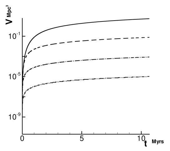
Figure 1: Ionized volume $V(t)$ vs. time $t$. The source intensities are taken to be $\dot{E}=5.8\times[10^{39}$ (dash dot dot), 10⁴¹ (dash dot), 10⁴³ (dash), and 10⁴⁵ (solid line)] erg sec^-1, and $\dot{N}$ to be 1.34$\times[10^{50}$, 10⁵², 10⁵⁴, and 10⁵⁶] sec^-1, respectively. Redshift is taken to be $1+z=10$.

Figure 1 shows a common feature for all sources that the growth of the ionized volume undergoes three phases: when $t$ is small, the growth is very fast, when $t$ is large the growth is very slow, and a transition phase between the fast and slow phases. The details of the growth are different for different sources. For a weak source with $\dot{E}=5.8\times 10^{39}$ erg s^-1, the ionized volume at the end of the fast growth phase is already comparable with that at later time. However, for a strong source with $\dot{E}=5.8\times 10^{45}$ erg s^-1 the ionized volume at the end of the fast growth phase is much smaller than that at later time. These features can be seen more clearly in Figure 2, which plots $d\ln V(t)/d\ln t$ vs. $\ln t$ for the same solutions in Figure 1. $d\ln V(t)/d\ln t$ is the index $a$ of the power-law relation $V\sim t^{a}$. Figure 2 shows once again the three phases of the power-law index. When $t$ is small, $d\ln V(t)/d\ln t\simeq 3$, or $V(t)\propto t^{3}$, and the radius of the ionized spheres, or the I-front, $r_{\rm I}=(3V/4\pi)^{1/3}\simeq ct$. Therefore, this actually is the fast or relativistic phase. In the transition phase, $d\ln V(t)/d\ln t$ decreases from 3 to about 1. Finally, $d\ln V(t)/d\ln t$ approaches to $\sim$ 1, or $r_{\rm I}\propto t^{1/3}$; this is the slow or non-relativistic phase.

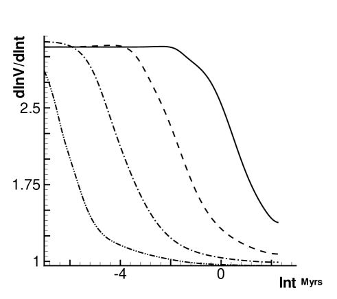
Figure 2: $d\ln V(t)/d\ln t$ vs. $\ln t({\rm Myrs})$ . The source intensities are taken to be $\dot{E}=5.8\times[10^{39}$ (dash dot dot), 10⁴¹ (dash dot), 10⁴³ (dash), and 10⁴⁵ (solid line)] erg sec^-1.

2.2 $\dot{E}$-dependence of the ionized region growth

We define a time scale, $t_{c}$, by $d\ln V(t)/d\ln t|_{t=t_{c}}=2.5$, which characterizes the transition time from the fast phase to the slow phase. The dependence of the time scale $t_{c}$ on $\dot{E}$ is plotted in Figure 3, which approximately follows $t_{c}\propto(\dot{E})^{1/2}$. Therefore, the transition time of the growth of the ionized volume is non-linearly dependent on the emission rate of the ionizing photon $\dot{E}$, which indicates that the growth of $V(t)$ also depends non-linearly on $\dot{E}$.

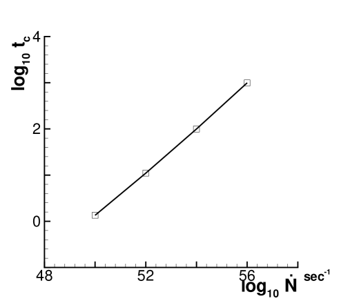
Figure 3: $\log_{10}(t_{c})$ vs. $\log_{10}{\dot{N}}({\rm sec}^{-1})$. Other parameters are the same as those in Figures 1 and 2. $t_{c}$ is in the unit of mean free flight time of ionized photons.

The non-linear dependence of $V(t)$ on $\dot{E}$ can be more prominently demonstrated by Figure 4, in which we plot the growth of the total ionized volume $V_{\rm total}(t)$ around one source with $\dot{E}=5.8\times 10^{45}$ erg s^-1, and those given by $m$ sources with intensity $5.8\times 10^{45}/m$ erg s^-1, with $m=10^{2}$, $10^{4}$ and $10^{6}$. Here we assume that the ionized regions for different sources do not overlap. Figure 4 shows that the growth rate of the ionized volume depends substantially on the number of sources, in spite of the fact that in all cases the total photon emission rate, $\dot{N}$, are the same. For a single strong source of $\dot{E}=5.8\times 10^{45}$ erg s^-1, $V_{\rm total}(t)$ at $t\simeq 1$ Myrs is only about 0.16, 0.10 and 0.08 of that from $m$ sources with intensities $\dot{E}=5.8\times 10^{45}/m$, erg s^-1 and $m=10^{2}$, $10^{4}$ and $10^{6}$.

Therefore, the larger the $t_{c}$, the less effective the ionization with the same rate $\dot{N}$. This is simply due to the retardation of photon propagation. In the period of $t<t_{c}$, the I-front propagates with about the speed of light $c$, and therefore, most photons emitted later will delay their contribution to the reionization by a time $t_{c}$. The longer the $t_{c}$, the longer the delay. When $t$ is larger than $t_{c}$, the speed of the I-front is slowing down and the later emitted photons start to join the reionization.

It is interesting to compare Figures 2 and 4. Figure 2 shows that the ionized volume growth velocity $d\ln V(t)/d\ln t$ approaches to 1 at $t\simeq 5$ Myrs for all sources with $\dot{E}\leq 5.8\times 10^{45}$ erg s^-1. However, Figure 4 shows that the total ionized volume $V_{\rm total,1\times 45}(t)$ of one source $\dot{E}=5.8\times 10^{45}$ erg s^-1 at 5 Myrs is still much less than the total ionized volume $V_{\rm total,m\times 45/m}(t)$ of $m$ ($>1$) sources with $\dot{E}=5.8\times 10^{45}/m$ erg s^-1. That is, the total ionized volume of one source $\dot{E}=5.8\times 10^{45}$ does not catch up with the total ionized volume of $m$ sources with $\dot{E}=5.8\times 10^{45}/m$ erg s^-1 even when they have about the same growth velocity $d\ln V(t)/d\ln t\simeq 1$. This is because $dV_{\rm total,m\times 39/m}/dt$ is larger than or equal to $dV_{\rm total,1\times 45}/dt$ for all time $0<t<t_{rec}$, we have $V_{\rm total,m\times 45/m}(t)-V_{\rm total,1\times 45}(t)=\int_{0}^{t}[dV_{\rm total,m\times 45/m}/dt-dV_{\rm total,1\times 45}/dt]dt>0$ in the period $t<t_{rec}$, i.e. before the ionized regions approach their Stromgren sphere. At $1+z=10$, $t_{rec}\simeq 8.6\times 10^{8}$ yrs, which is comparable with $1/H$, and therefore part of the UV photons from strong sources may cause ionization when the sources have already ceased. Comparing with weak sources, the reionization of strong sources such as $\dot{E}\geq 10^{45}$ erg s^-1 is less effective at the period $t<t_{rec}$.

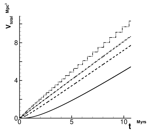
Figure 4: Evolution of $V_{\rm total}(t)$. The source intensities are taken to be $\dot{E}=5.8\times[10^{39}$ (dash dot dot), 10⁴¹(dash dot), 10⁴³ (dash), and 10⁴⁵ (solid line)] erg sec^-1.

2.3 Inhomogeneous distribution of gas

Figure 5: The evolution of $V_{\rm total}(t)$ for the number density distribution given by eq.(2). The source intensities are taken to be $\dot{E}=5.8\times[10^{39}$ (dash dot dot), 10⁴¹ (dash dot), 10⁴³ (dash), and 10⁴⁵ (solid line)] erg sec^-1.

Generally, the mass density of gas is high near the source. To study its effect, we assume the density distribution $n(r)$ is given by

$$\frac{n(r)}{n_{0}}=1+\frac{n_{c}}{n_{0}}e^{-r/R},$$ (2)

where $R$ is the size of the high density region, and $n_{c}/n_{0}$ is the density increase in the center of the sources. As an example, we choose $(n_{c}/n_{0})=10$ and $R=50$ in the unit of the mean free path of the ionization photons. The growth of the ionized volume from different intensity of sources is plotted in Figure 5, which shows the similar behavior as that in Figure 4. Quantitatively, the high density core of $n_{r}/n_{0}=10$ and $R=50$ plays a similar role as a sphere with size 500 in the unit of mean free path. We have also calculated the evolution using other inhomogeneous density models and have obtained results similar to those in Figure 5.

3 Clustered point sources

3.1 Time scale with the merged ionized regions

The UV photon sources of the first generation of stars may not be very strong, however, they are most likely clustered. The merging of ionized regions around a single source will lead to complicated configuration of the ionized regions of clustered sources. However, in terms of the growth rate of the ionized volume, the problem is simplified. The merging process of clustered ionized regions can approximately be decomposed into a set of two-region merging. It is similar to the identification of clusters by the friend-of-friend method. Therefore, we may reveal some common features of the merging effect on the ionized volume growth rate by a detailed study of the merging of two ionized regions.

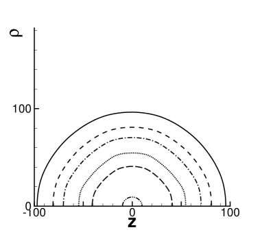
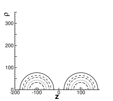
Figure 6: The evolution of the ionized region ($f_{\rm HI}(\rho,z,t)<0.90$) of two UV photon sources with intensity $\dot{E}=0.5\times 5.8\times 10^{41}$ erg s^-1. The contours from small to large correspond, respectively, to the time $t^{\prime}$ = 10 (dash dot dot), 100 (long dash), 200 (dot), 400 (dash dot), 600 (dash), 1000 (solid) in the unit of the mean free flight time. $\rho$ and z are dimensionless, i.e. in the unit of mean free path of ionizing photons. The distance between the two sources is $a=1$ (top), 10 (middle) and 100 (bottom) also in the unit of mean free path of ionizing photons.

Let us consider two sources located, respectively, at $(x,y,z)=(0,0,a)$ and $(0,0,-a)$. We calculate the time-dependence of the profile of the ionized regions around the two sources. The evolution of the profiles of the ionized region in the $\rho-z$ plane ($\rho=\sqrt{x^{2}+y^{2}}$) is shown in Figure 6, where the variables $\rho$ and $z$ are dimensionless as defined in §2.1. The ionized region is still defined by the region in which $f_{\rm HI}(\rho,z,t)<0.9$. In Figure 6, the intensities of the two sources are taken to be $\dot{E}=0.5\times 5.8\times 10^{41}$ erg s^-1, and $a=1$, 10 and 100 in the unit of mean free path of the ionizing photons. For each case, the profiles are at the time $t^{\prime}=10,100,200,400,600,1000$ in the unit of the mean free flight time.

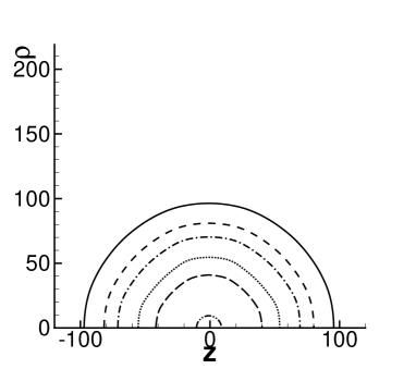
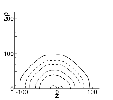
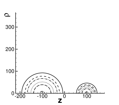
Figure 7: The evolution of the ionized region ($f_{\rm HI}(\rho,z,t)<0.90$) of two UV photon sources with intensities $\dot{E}=0.9\times 5.8\times 10^{41}$ and $0.1\times 5.8\times 10^{41}$ erg s^-1. The contours from small to large sizes correspond, respectively, to the time $t^{\prime}$ = 10, 100, 200, 400, 600, 1000 in the unit of the mean free flight time. $\rho$ and z are in units of mean free path of ionizing photons. The distance between the two sources is $a=1$ (top), 10 (middle) and 100 (bottom) in the unit of mean free path of ionizing photons.

From Figure 6, one can see first that the configuration of the ionized regions is very different from the ionized sphere of a point source. In the case of $a=1$, the ionized regions have already merged when $t^{\prime}<10$, and the profile of the merged ionized region is like a sphere. For $a=10$, there are two spheres around the two sources when $t^{\prime}<10$, and they merge at $t^{\prime}<100$. The profile of the merged ionized region is no longer spherical. For $a=100$, however, no merging occurs even at the time $t^{\prime}\simeq 1000$. This is simply because the time scale $t_{c}$ of sources with $\dot{E}=0.5\times 5.8\times 10^{41}$ erg s^-1 is $\simeq 30$. If the distance between the two sources is less than $ct_{c}$, the merging is realized in the fast phase. On the other hand, for $a=100$, which is larger than $ct_{c}$, the merging time will be much larger than $a/c$.

In Figure 7, we show the evolution of the ionized profiles for two sources located, respectively, at $(x,y,z)=(0,0,a)$ and $(0,0,-a)$ with intensities $\dot{E}=0.9\times 5.8\times 10^{41}$ and $\dot{E}=0.1\times 5.8\times 10^{41}$ erg s^-1. Similar to Figure 6, in the case of $a=1$, the ionized regions have merged when $t<10$, and the profile of the merged ionized region is like a sphere. For $a=10$, there are two spheres around the two sources when $t<10$, and they merge at $t<100$. There is no merging for the case of $a=100$ even when the time is as large as $t\simeq 1000$. Therefore, the basic feature of Figure 7 is the same as that in Figure 6: for two sources with the transition time $t_{1c}$ and $t_{2c}$, if their distance $2a$ is less than $c[t_{1c}+t_{2c}]$, the merging occurs quickly, while it will be very slow if $2a>c[t_{1c}+t_{2c}]$.

From the middle panel of Figure 7, it is interesting to see that the two ionized spheres have about the same size, although the intensities of the two sources are different by a factor of about 10. This is because in the fast phase, the growth of the ionized sphere radius is given by the speed of light, regardless of the intensity of the sources.

3.2 Growth of the ionized regions of two sources

For the two source case, the configuration of the ionized regions generally is very different from the spherical ionized region of a point source. What we want to show in this section is, however, that the growth of the total ionized volume, $V(t)$, of two sources with intensities $\dot{E}_{1}$ and $\dot{E}_{2}$ is the same as that of a single source of $\dot{E}=\dot{E}_{1}+\dot{E}_{2}$ if the distance between the two sources $2a$ is less than $c(t_{1c}+t_{2c})$, with $t_{1c}$ and $t_{2c}$ being the transition time scales of the two sources, respectively. If $2a$ is larger than $c(t_{1c}+t_{2c})$, the effect of the merging is small, and the growth of the total ionized volume of the two sources can basically be treated as two isolated ionized regions, i.e. its growth rate should be faster than that of the single source of $\dot{E}=\dot{E}_{1}+\dot{E}_{2}$.

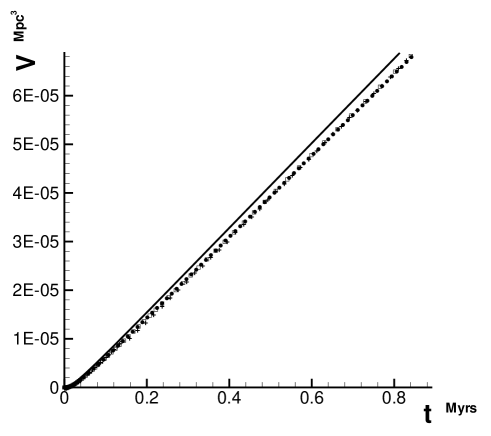
Figure 8: Ionized volume $V(t)$ vs. time $t$ of two sources with the same parameters as those in Figure 6. $a=100$, 10 and 1 are shown, respectively, by solid line, filled circles and crosses. The unfilled square symbols are for the single point source with $\dot{E}=\dot{E}_{1}+\dot{E}_{2}$.

Figure 8 plots the evolution of $V(t)$ of two sources with parameters $\dot{E}_{1}$ and $\dot{E}_{2}$ as those used in Figure 6 of the last section. The $V(t)$ of a single source with intensity $\dot{E}=\dot{E}_{1}+\dot{E}_{2}$ is also given in Figure 8. From Figure 3, we know that for $a=1$ and 10, $2a$ is less than $c(t_{1c}+t_{2c})$, while for $a=100$, $2a$ is larger than $c(t_{1c}+t_{2c})$. Figure 8 indeed shows clearly that the growth of the total ionized volume of $a=100$ is faster than that of $a=1$ and 10, although the source intensity of $a=100$ is the same as that of $a=1$ and 10. The growth of the ionized volume of the cases $a=1$ and 10 are the same. They are also exactly the same as the $V(t)$ of a single source with intensity $\dot{E}=\dot{E}_{1}+\dot{E}_{2}$, though the configuration of the ionized regions of two sources is very different from that of a single point source.

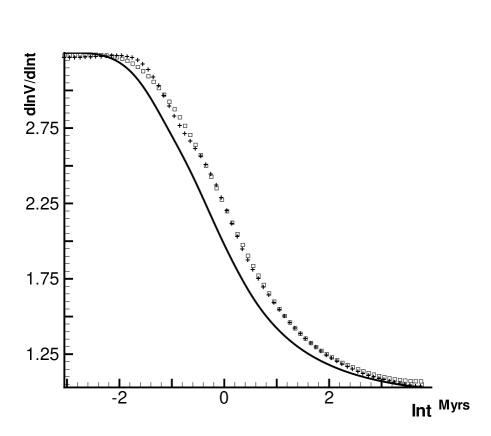
Figure 9: $d\ln V(t)/d\ln t$ vs. $\ln t$ (variable $t$ is dimensionless) of two sources with intensity $\dot{E}=(1/2)5.8\times 10^{41}$ erg s^-1 at $a=1$ (cross) and 100 (solid). The unfilled square symbols are for a single source with $\dot{E}=5.8\times 10^{41}$ erg s^-1.

In Figure 9 we plot $d\ln V(t)/d\ln t$ vs. $\ln t$ of the two sources in Figure 8. Similar to Figure 2, the evolution of $d\ln V(t)/d\ln t$ generally consists of three phases: the fast growth phase, when $t$ is small, $d\ln V(t)/d\ln t\simeq 3$, the transition phase, and the slow growth phase, when $t$ is large, $d\ln V(t)/d\ln t$ approaches to $\sim$ 1. For the ionized region of two sources, one can not define the I-front with the radius of the ionized region, because the ionized region is no longer spherical. However, $d\ln V(t)/d\ln t\simeq 3$ tells us that the length scale of the non-spherical ionized region should increase with the speed of $\simeq c$.

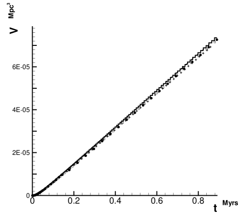
Figure 10: Ionized volume $V(t)$ vs. time $t$ of two sources with the same parameters as those in Figure 7. $a=100$, 10 and 1 are shown, respectively, by solid line, filled circle symbols and cross symbols. The unfilled square symbols are for a single point source with $\dot{E}=\dot{E}_{1}+\dot{E}_{2}$.

As expected, Figure 9 shows that the transition time scale $t_{c}$ of the case $a=100$ is shorter than that of the cases $a=1$ and 10. Figure 9 presents also the curve of $d\ln V(t)/d\ln t$ vs. $\ln t$ of the single point source with $\dot{E}=\dot{E}_{1}+\dot{E}_{2}$, which is almost identical with the curve of $a=1$. Therefore, we can conclude that in terms of the growth of the ionized volume, two sources with distance $a=1$ and 10 are equal to a single point source with $\dot{E}=\dot{E}_{1}+\dot{E}_{2}$.

Figure 10 is similar to Figure 8, but for the two sources with parameters used in Figure 7. In this case, most UV photons come from source 1 with $\dot{E}=0.9\times 5.8\times 10^{41}$ erg s^-1, and the intensity of source 2 $\dot{E}=0.1\times 5.8\times 10^{41}$ erg s^-1 is much smaller than that of source 1. Nevertheless, we still can see that the growth of the total ionized volume of $a=100$ is faster than that of $a=1$ and 10. The growth of the ionized volume of the cases $a=1$ and 10 are the same, and it is also the same as that of the single source with intensity $\dot{E}=\dot{E}_{1}+\dot{E}_{2}$.

Figure 11: $d\ln V(t)/d\ln t$ vs. $\ln t$ (variable $t$ is dimensionless) of two sources with intensity $\dot{E}=0.9\times 5.8\times 10^{41}$ and $0.1\times 5.8\times 10^{41}$ erg s^-1 at $a=1$ (cross) and 100 (solid). The unfilled square symbols are for a single source with $\dot{E}=5.8\times 10^{41}$ erg s^-1.

Figure 11 is similar to Figure 9, but for the two sources shown in Figure 10. Similar to Figure 9, the transition time scale $t_{c}$ of the case $a=100$ is shorter than that of the cases $a=1$ and 10. The curve of $d\ln V(t)/d\ln t$ vs. $\ln t$ for $a=1$ is almost identical to the curve of a single point source with $\dot{E}=\dot{E}_{1}+\dot{E}_{2}$.

Thus, in terms of the growth of the ionized volume, once the two sources $\dot{E}_{1}$ and $\dot{E}_{2}$ have a distance $<c(t_{1c}+t_{2c})$, one can replace them by a single source of $\dot{E}=\dot{E}_{1}+\dot{E}_{2}$. Furthermore, one may apply the merging of two sources to multi-sources. In other words, in a cluster of sources, we can use the so-called friend-of-friend method to identify all the sources, for which the distances between all the nearest neighbors $i$ and $j$ are smaller than $c(t^{i}_{c}+t^{j}_{c})$, $t^{i}_{c}$ being the time scale $t_{c}$ of source $i$. That is, for each point source, we plot a sphere around the source with radius $ct_{c}$ corresponding to its intensity, two sources with overlapped spheres can be identified as a cluster consisting of the two sources. Repeatedly applying the method to each pair of sources, one can then identify a cluster consisting of all the sources of which the $ct_{c}$ spheres are connected. For this cluster, the ionized volume growth can be approximately described by a single source of $\dot{E}=\sum_{i}\dot{E}_{i}$, where $\dot{E}_{i}$ is the intensity of source $i$.

4 Discussion and conclusion

We have developed the WENO algorithm to solve radiative transfer equation beyond one physical dimension, which can precisely reveal the features of the merging of the ionized regions of UV photon sources.

We show that the growth of the ionized volume around either one or two point sources generally consists of three phases: fast growth phase at the early evolution, slow growth phase at the later evolution, and a transition phase between them. The transition time $t_{c}$ depends significantly on the intensity of the photon sources $\dot{E}$, approximately to be $t_{c}\propto\dot{E}^{1/2}$. Most of the photons emitted by the ionizing sources would be delayed a time $t_{c}$ to contribute to the ionization. The longer the $t_{c}$ the less effective the ionization. Consequently, linear superposition is not available in estimating the ionized volume. The growth of the ionized volume of multiple isolated sources $\dot{E}_{i}$ ($i=1,2,\dots$) generally is much faster than that of a single source with intensity $\dot{E}=\Sigma_{i}\dot{E}_{i}$.

Therefore, to calculate accurately the growth of the ionized volume at $t$, one should not use eq.(1), but take into account of the retardation of UV photons. This effect is more substantial if the first generation of stars are highly clustered. If the ionized spheres of these sources are merging in relativistic growth phase, the cluster would behave as a single source with intensity equal to the summation of intensities of these sources. Therefore, tight clustering of UV sources will delay the development of reionization.

These results may already be useful in studying the 21 cm signals from the reionization epoch. It has been shown that a 21 cm emission and absorption region will develop around a point source once the speed of the ionization front (I-front) is significantly lower than the speed of light (Liu et al. 2007). The 21 cm region extends from the I-front to the front of light $(r=ct)$; its inner part is the emission region and its outer part is the absorption region. Therefore, the 21 cm region should be formed only at the time $t>t_{c}$. Since sources with weak intensity have small $t_{c}$, while strong sources or tight clusters of weak sources have longer $t_{c}$, sources with weak intensity produce 21 cm signal earlier, while strong sources, or tightly clustered weak sources produce it later. The results calculated from equation (1) will over-predict the ionization, and thus lead to less 21 cm signals. These features could be important to reconstruct the history of reionization with 21 cm tomography and/or cross correlation between redshifted 21 cm signals and emission on other bands from the center of the sources.

Acknowledgments.

This work is supported in part by the US NSF under the grants AST-0506734 and AST-0507340. J.R.Liu is supported partially by the ICRAnet.

Appendix A Equation

The radiative transfer equation in an expanding universe is (Bernstein, 1988; Qiu et al. 2006)

$${\partial J\over\partial\,(ct)}+\frac{1}{a}\nabla\cdot{\bf n}J+{\partial\over\partial\omega}(HJ)=-(k_{\nu}+3H)J+S,$$ (3)

where $J(t,{\bf x},\nu,{\bf n})$ is the specific intensity, $a$ is the cosmic factor, $H=\dot{a}/a$, $\nu$ is the frequency of photon, $\omega\equiv\ln 1/\nu$, and ${\bf n}$ is a unit vector in the direction of the photon propagation. We take $c=1$ below. The absorption coefficient $k_{\nu}$ is

$$k_{\nu}=\sigma(\nu)n_{{\rm HI}}(t,{\bf x})$$ (4)

where the cross section $\sigma(\nu)=\sigma_{0}(\nu_{0}/\nu)^{3}$ and $\sigma_{0}=6.3\times 10^{-18}$ cm².

Assuming that the point sources $i$ ($i=1,\dots,n$) are located at $x_{i}$, and all photons are emitted along the radial direction, we have

$$S(t,{\bf x},{\nu},{\bf n})=\sum_{i=1}^{n}f_{i}(t,{\bf x},\nu)\delta({\bf n-e_{r_{i}}}),$$ (5)

where ${\bf e_{r_{i}}}$ is the unit radial vector with respect to ${\bf x}_{i}$. The function $f_{i}$ is given by

$$f_{i}(t,{\bf x},\nu)=\left\{\begin{array}[]{ll}\dot{E}_{i}(\nu)/V,&{\rm at\ {\bf x}={\bf x_{i}}}\\ 0,&{\rm otherwise},\end{array}\right.$$ (6)

where $\dot{E}_{i}(\nu)$ is the energy of photons emitted from the sources $i$ per unit time at frequency $\nu$. When $V\rightarrow 0$, $f_{i}(t,{\bf x},\nu)\rightarrow\dot{E}_{i}\delta({\bf x}_{i})$. We assume the energy spectrum of UV photons to be of a power law $\dot{E}(\nu)=\dot{E_{0}}(\nu_{0}/\nu)^{\alpha}$, and $\nu_{0}$ is the ionization energy of the ground state of hydrogen $h\nu_{0}=13.6$ eV. Integration of $\dot{E}$ over $\nu$ gives the total intensity (energy per unit time) of ionizing photons emitted by the source, $\dot{E}=\int_{\nu_{0}}^{\infty}\dot{E}(\nu)d\nu=\dot{E}_{0}\nu_{0}/(\alpha-1)$.

Since there is no photon-photon collision, the solution of eq.(3) can be written as

$$J=\sum_{i=1}^{n}J_{i}\delta({\bf n-e_{r_{i}}})$$ (7)

and $J_{i}$ satisfies following equation

$${\partial J_{i}\over\partial\,t}+\nabla\cdot{\bf e_{r_{i}}}J_{i}=-k_{\nu}J_{i}+f_{i}.$$ (8)

The coupling among $J_{i}$ is via the absorption coefficient $k_{\nu}$ defined in eq.(4). The evolution of the number density of neutral hydrogen, $n_{\rm HI}(t,{\bf x})$, is governed by the ionization equation,

$$\frac{df_{\rm HI}}{dt}=\alpha_{\rm HII}n_{e}f_{\rm HII}-\Gamma_{\rm\gamma HI}f_{\rm HI}-\Gamma_{\rm eHI}n_{e}f_{\rm HI}$$ (9)

where the fraction of neutral hydrogen $f_{\rm HI}\equiv n_{\rm HI}(t,{\bf x})/n({\bf x})$, $n({\bf x})$ is the hydrogen distribution, and $n_{e}=n({\bf x})-n_{\rm HI}(t,{\bf x})$ is the number density of electrons, if the electrons from ionized helium can be ignored. $\alpha_{\rm HII}$ is the recombination coefficient, $\Gamma_{\rm eHI}$ is the collision ionization rate, and the photoionization rate $\Gamma_{\rm\gamma HI}(t,\rho,z)$ is given by

$$\Gamma_{\gamma{\rm HI}}(t,{\bf x})=\sum_{i=1}^{n}\int_{\nu_{0}}^{\infty}d\nu\frac{J_{i}(t,{\bf x},\nu)}{h\nu}\sigma(\nu).$$ (10)

The evolution of the hydrogen gas temperature $T$, in the unit of K, is given by

$$\frac{dU}{dt}=H-n^{2}C,$$ (11)

where $U=\frac{3}{2}nk_{B}T$ with $k_{B}$ be the Boltzmann constant, and

$$H=n_{\rm HI}\sum_{i=1}^{n}\int_{\nu_{0}}^{\infty}J_{i}(t,{\bf x},\nu)\sigma(\nu)\frac{\nu-\nu_{0}}{\nu}d\nu.$$ (12)

The relevant parameters are as follows (Theuns et al. 1998)

1. The recombination coefficient

$$\alpha_{\rm HII}=6.30\times 10^{-11}T^{-1/2}T_{3}^{-0.2}/(1+T^{0.7}_{6}),$$ (13)

where $T$ is temperature, and $T_{n}=T/10^{n}$.

2. The collision ionization

$$\Gamma_{\rm eHI}=1.17\times 10^{-10}T^{1/2}e^{-157809.1/T}(1+T_{5}^{1/2})^{-1}.$$ (14)

3. The cooling. Since only the recombination cooling is important, we have

$$C = 8.70\times 10^{-27}T^{1/2}T_{3}^{-0.2}(1+T_{6}^{0.7})^{-1}[1-f_{\rm HI}]^{2}$$

$$+ 1.42\times 10^{-27}T^{1/2}[1-f_{\rm HI}]^{2}$$

$$+ 2.45\times 10^{-21}T^{1/2}e^{-157809.1/T}(1+T_{5}^{1/2})^{-1}(1-f_{\rm HI})f_{\rm HI}$$

$$+ 7.5\times 10^{-19}e^{-118348/T}(1+T_{5}^{1/2})^{-1}(1-f_{\rm HI})f_{\rm HI}$$

where $T_{n}=T/10^{n}$. The terms on the r.h.s. of eq.(A) are, respectively, the recombination cooling, the collisional ionization cooling, the collisional excitation cooling and bremsstrahlung. Both $H$ and $C$ are in the unit of ergs cm³ s^-1.

Appendix B Two sources

Consider the case of two sources. Using cylindrical coordinate $(\rho,\theta,z)$, the two sources are assumed to be located at ${\bf x}={\bf x}_{\pm}=(0,0,a)$, with ${\bf e}_{r_{\pm}}=(\rho/\sqrt{\rho^{2}+(z\mp a)^{2}},0,(z\mp a)/\sqrt{\rho^{2}+(z\mp a)^{2}})$. The corresponding radiative transfer equations eq.(8) are

$${\partial J_{\pm}\over\partial\,t}+\frac{1}{\rho}\frac{\partial}{\partial\rho}\left(\frac{\rho^{2}}{\sqrt{\rho^{2}+(z\mp a)^{2}}}J_{\pm}\right)+\frac{\partial}{\partial z}\left(\frac{(z\mp a)}{\sqrt{\rho^{2}+(z\mp a)^{2}}}J_{\pm}\right)$$

$$\hskip 85.35826pt=-k_{\nu}J_{\pm}+f_{\pm},$$

where $J_{\pm}(t,\rho,z,\nu)$ are the specific intensities for sources ${\bf x_{\pm}}$.

Instead of adding the source term $f_{\pm}$ in the r.h.s of eq.(B), equivalently, we impose a boundary condition

$$\lim_{\rho\rightarrow 0,z\rightarrow\pm a}4\pi r_{\pm}^{2}J_{\pm}(t,\rho,z,\nu)=\dot{E}_{\pm}(\nu),$$ (17)

where $r_{\pm}=\sqrt{\rho^{2}+(z\mp a)^{2}}$, $\dot{E}(\nu)=\dot{E_{0}}_{\pm}(\nu_{0}/\nu)^{\alpha}$ is the energy of photons emitted from the sources per unit time at frequency $\nu$.

The absorption coefficient in eq.(B) $k_{\nu}$ is defined in eq.(4), with $n_{\rm HI}(t,\rho,z)\equiv nf_{\rm HI}(t,\rho,z)$ governed by the ionization equation eq.(9). Here the photoionization rate $\Gamma_{\rm\gamma HI}(t,\rho,z)$ in eq.(9) is given by

$$\Gamma_{\rm\gamma HI}(t,\rho,z)=\int_{\nu_{0}}^{\infty}d\nu\frac{J_{+}(t,\rho,z,\nu)+J_{+}(t,\rho,z,\nu)}{h\nu}\sigma(\nu).$$ (18)

The kinetic temperature of the baryon gas is determined by eq.(11) with

$$H=n_{\rm HI}\int_{\nu_{0}}^{\infty}(J_{+}(t,\rho,z,\nu)+J_{-}(t,\rho,z,\nu))\sigma(\nu)\frac{\nu-\nu_{0}}{\nu}d\nu.$$ (19)

Appendix C The numerical algorithm

In this paper, we are solving the system of equations (B), (9) and (11). To apply the WENO algorithm, we rewrite eq.(B) into a conservative form as

$$\frac{\partial J_{\pm}}{\partial t}+\frac{\partial}{\partial\rho}[\frac{\rho}{r_{\pm}}J_{\pm}]+\frac{\partial}{\partial z}[\frac{z\mp a}{r_{\pm}}J_{\pm}]=-\frac{1}{r_{\pm}}J_{\pm}-k_{\nu}J_{\pm},$$ (20)

where $r_{\pm}=\sqrt{\rho^{2}+(z\mp a)^{2}}$. We use the WENO algorithm to approximate the spatial derivatives in eq.(20) (Qiu et al. 2006).

In the numerical implementation, it is convenient to introduce the dimensionless variables $t^{\prime}$, $\rho^{\prime}$, $z^{\prime}$, $a^{\prime}$, $\nu^{\prime}$, $J^{\prime}$ by rescaling $t^{\prime}=cn\sigma_{0}t$, $\rho^{\prime}=n\sigma_{0}\rho$, $z^{\prime}=n\sigma_{0}z$, $a^{\prime}=n\sigma_{0}a$, $\nu^{\prime}=\nu/\nu_{0}$, and $J^{\prime}_{\pm}d\nu^{\prime}=\frac{\sigma_{0}}{h\nu_{0}n}J_{\pm}d\nu$. Therefore, $t^{\prime}$ and $r^{\prime}$ are respectively, the time and distance in the units of mean free flight time and mean free path of ionizing photon $h\nu_{0}$ in the non-ionized background hydrogen gas $n$. For the $\Lambda$CDM model, $n=1.88\times 10^{-7}(1+z)^{3}$ cm^-3, where $z$ is the redshift, $t=0.89(1+z)^{-3}t^{\prime}$ Myrs and $r=0.27(1+z)^{-3}r^{\prime}$ Mpc. Then the system of equations (20), (9) and (11) can be rewritten as the following system

$$\frac{\partial J^{\prime}_{\pm}}{\partial t^{\prime}}+\frac{\partial}{\partial\rho^{\prime}}[\frac{\rho^{\prime}}{r^{\prime}_{\pm}}J^{\prime}_{\pm}]+\frac{\partial}{\partial z^{\prime}}[\frac{z^{\prime}\mp a^{\prime}}{r^{\prime}_{\pm}}J^{\prime}_{\pm}]=-\frac{1}{r^{\prime}_{\pm}}J^{\prime}_{\pm}-\frac{1}{\nu^{\prime 3}}f_{HI}J^{\prime}_{\pm}$$ (21)

$$c\sigma_{0}\frac{df_{HI}}{dt^{\prime}}=\alpha_{HII}(1-f_{HI})^{2}-\frac{\Gamma_{\gamma HI}}{n}f_{HI}-\Gamma_{eHI}(1-f_{HI})f_{HI}$$ (22)

$$\frac{3}{2}c\sigma_{0}k_{B}\frac{\partial T}{\partial t^{\prime}}=H-C$$ (23)

with $\frac{\Gamma_{\gamma HI}}{n}$ given by

$$\frac{1}{n}\Gamma_{\gamma HI}(t,\rho,z)=\int_{1}^{\infty}\frac{J^{\prime}_{+}+J^{\prime}_{-}}{\nu^{\prime 4}}d\nu^{\prime},$$ (24)

$H$ given by

$$H=h\nu_{0}f_{HI}\int_{1}^{\infty}(J^{\prime}_{+}+J^{\prime}_{-})\frac{\nu^{\prime}-1}{\nu^{\prime 4}}d\nu^{\prime},$$ (25)

and $\alpha_{HII}$, $\Gamma_{eHI}$ and $C$ given by equations (13), (14) and (A) respectively.

To solve the radiative transfer equation (21), we adopt the fifth-order finite difference WENO scheme, which was designed in (Jiang $\&$ Shu 1996), coupled with the third order TVD Runge-Kutta time discretization for the system of equations (21), (22) and (23). The multi-time-scale strategy (Qiu et al. 2007) and the adaptive time step strategy (Liu et al. 2007) are used to save the increased computational cost introduced by the stiffness of the equations (22) and (23). The numerical algorithms are implemented as describe below. For the sake of simplicity, we drop the prime in the notations. For example, $J$ means $J^{\prime}$ hereafter.

• The computational domain and computational mesh:

  The computational domain is $(\rho,z,\nu)\in[0,\rho_{max}]\times[-z_{max},z_{max}]\times[1,\nu_{max}]$, where $\rho_{max}$ and $z_{max}$ are chosen such that $J(t,\rho,z,\nu)\approx 0$ for $\rho>\rho_{max}$, $|z|>z_{max}$ or $\nu>\nu_{max}$. In our computation, $\rho_{max}$ is taken to be greater than the final computational time t, $z_{max}$ is taken to be $\rho_{max}+a$ and $\nu_{max}=10^{6}$.

  To avoid $r_{\pm}$ in eq. (21) to become 0, we design the computational mesh, such that ${\bf x_{\pm}}$ are located at the center between grid points. The mesh sizes in the $\rho$- and $z$- directions are set to be the same, i.e. $\Delta\rho=\Delta z$, to preserve the spherical symmetry property of the numerical solution before the merging of the two sources. The mesh in the $\nu$ direction is taken to be smooth but not uniform. Specifically, the mesh sizes are designed as the following

  $$\Delta z=\frac{a}{N_{z_{a}}+\frac{1}{2}};\quad\Delta\rho=\Delta z;\quad\Delta\xi=\log_{2}{\nu_{max}}/N_{\nu};$$

  with $N_{z_{a}}$ being the number of mesh points in [0, a] in the $z$-direction, and $N_{\nu}$ being the number of mesh points in the $\nu$-direction. The computational mesh is

  $$\rho_{i}=\left(i-\frac{1}{2}\right)\Delta\rho,\quad i=1,2,...,N_{\rho},$$

  $$z_{j}=j\Delta z,\quad j=1,2,...,N_{z},$$

  $$\nu_{k}=2^{\xi_{k}},\quad with\quad\xi_{k}=k\Delta\xi,\quad k=1,2,...,N_{\nu}.$$

• The WENO method in approximating the spatial derivatives:

  The approximation to the point values of the solution $J_{\pm}(t^{n},\rho_{i},z_{j},\nu_{k})$, denoted by $J^{n}_{\pm,i,j,k}$, is obtained with a dimension by dimension approximation to the spatial derivatives using the fifth order WENO scheme (Jiang $\&$ Shu 1996). Taking $\frac{\partial}{\partial z}(\frac{z-a}{r_{+}}J_{+})$ as an example, the approximation is performed along the $z$-line with fixed $\rho_{i}$ and $\nu_{k}$:

  $$\frac{\partial}{\partial z}\left(\frac{z_{j}-a}{r_{+}(\rho_{i},z_{j})}J_{+}(t^{n},\rho_{i},z_{j},\nu_{k})\right)\approx\frac{1}{\Delta z}(\hat{h}_{j+1/2}-\hat{h}_{j-1/2})$$ (26)

  where the numerical flux $\hat{h}_{j+\frac{1}{2}}$ is obtained with the following procedure. When the “wind direction”, namely the coefficient $\frac{z_{j}+z_{j+1}}{2}-a$ is positive at the mesh boundary, we use a left-biased stencil in reconstructing the numerical flux $\hat{h}_{j+\frac{1}{2}}$ as described in detail below. When the “wind direction” is negative, we use a right-biased stencil to obtain the numerical flux $\hat{h}_{j+\frac{1}{2}}$, following a mirror symmetry reconstruction with respect to $j+\frac{1}{2}$ as that of the left-biased stencil. When the coefficient $\frac{z_{j}+z_{j+1}}{2}-a$ = 0, which actually will happen due to the way we design our mesh, the numerical flux is simply set to be 0.

  We denote

  $${h_{j}}=J(t^{n},\rho_{i},z_{j},\nu_{k}),\qquad j=-2,-1,...,{N_{z}}+2$$

  where $n$, $i$ and $k$ are fixed. The numerical flux from the regular WENO procedure is obtained by

  $$\hat{h}_{j+1/2}=\omega_{1}\hat{h}_{j+1/2}^{(1)}+\omega_{2}\hat{h}_{j+1/2}^{(2)}+\omega_{3}\hat{h}_{j+1/2}^{(3)}$$

  where $\hat{h}_{j+1/2}^{(m)}$ are the three third order fluxes on three different stencils given by

  $$\hat{h}_{j+1/2}^{(1)} = \frac{1}{3}h_{j-2}-\frac{7}{6}h_{j-1}+\frac{11}{6}h_{j},$$

  $$\hat{h}_{j+1/2}^{(2)} = -\frac{1}{6}h_{j-1}+\frac{5}{6}h_{j}+\frac{1}{3}h_{j+1},$$

  $$\hat{h}_{j+1/2}^{(3)} = \frac{1}{3}h_{j}+\frac{5}{6}h_{j+1}-\frac{1}{6}h_{j+2},$$

  and the nonlinear weights $\omega_{m}$ are given by

  $$\omega_{m}=\frac{\tilde{\omega}_{m}}{\sum_{l=1}^{3}\tilde{\omega}_{l}},\qquad\tilde{\omega}_{l}=\frac{\gamma_{l}}{(\varepsilon+\beta_{l})^{2}},$$

  with the linear weights $\gamma_{l}$ given by

  $$\gamma_{1}=\frac{1}{10},\qquad\gamma_{2}=\frac{3}{5},\qquad\gamma_{3}=\frac{3}{10},$$

  and the smoothness indicators $\beta_{l}$ given by

  $$\beta_{1} = \frac{13}{12}\left(h_{j-2}-2h_{j-1}+h_{j}\right)^{2}+\frac{1}{4}\left(h_{j-2}-4h_{j-1}+3h_{j}\right)^{2}$$

  $$\beta_{2} = \frac{13}{12}\left(h_{j-1}-2h_{j}+h_{j+1}\right)^{2}+\frac{1}{4}\left(h_{j-1}-h_{j+1}\right)^{2}$$

  $$\beta_{3} = \frac{13}{12}\left(h_{j}-2h_{j+1}+h_{j+2}\right)^{2}+\frac{1}{4}\left(3h_{j}-4h_{j+1}+h_{j+2}\right)^{2}.$$

  $\varepsilon$ is a parameter to avoid the denominator to become 0 and is taken as $\varepsilon=10^{-5}$ times the maximum magnitude of the initial condition $J$ in the computation.

• Time integration:

  To evolve in time, we use the third order TVD Runge-Kutta method (Shu $\&$ Osher 1988). For systems of ODEs ${u}_{t}=L({u})$, the third order Runge-Kutta method is

  $$u^{(1)} = u^{n}+\Delta tL(u^{n},t^{n})$$ (27)

  $$u^{(2)} = \frac{3}{4}u^{n}+\frac{1}{4}(u^{(1)}+\Delta tL(u^{(1)}))$$ (28)

  $$u^{n+1} = \frac{1}{3}u^{n}+\frac{2}{3}(u^{(2)}+\Delta tL(u^{(2)}))$$ (29)

  The difficulty of the direct implementation of the Runge-Kutta method lies in the stiffness of equations (22) and (23). Especially for the strong source, one needs a very small time step $\Delta t$, as small as $10^{-7}$, to guarantee the stability of the numerical scheme, therefore the computational cost for long time integration is huge. In this paper, we adapt the multi-time-scale strategy (Qiu et al. 2007) and the adaptive-time-step strategy (Liu et al. 2007) to evolve the system of equations in time. We refer to (Qiu et al. 2007) and (Liu et al. 2007) for the details of its implementation.

• Numerical boundary condition:

  • In the $\rho$-direction,
    at $\rho=0$,

    $$J_{\pm,-i,j,k}=J_{\pm,i+1,j,k},\quad i=0,1,2,$$

    at $\rho=\rho_{max}$,

    $$J_{\pm,N_{\rho}+i,j,k}=0,\quad i=0,1,2.$$

  • In the $z$-direction,
    at $z=\mp z_{max}$,

    $$J_{\pm,i,\mp(N_{z}+i),k}=0,\quad i=0,1,2$$

  • Around the point sources ${\bf x_{\pm}}$, according to eq.(17),
    

    $$J_{\pm,i,j,k}=\frac{1}{\nu_{k}^{\alpha}}\frac{\dot{E}}{4\pi r^{2}_{\pm,i,j}},\quad r_{\pm,i,j}<r_{s}$$

    with $r_{\pm,i,j}=\sqrt{\rho_{i}^{2}+(z_{j}\mp a)^{2}}$. $r_{s}$ is a small number depending on the mesh size. $r_{s}$ is bigger when the mesh is coarser.

• Parallel computing:

  The computational cost in solving the system of equations (21), (22) and (23) is quite large for this 3-dimensional (2-D in the physical space and 1-D in the frequency space) time dependent problem. Parallel computing with mpif77 is used to speed up the computation.

References

- (1) Abel, T., Norman, M.L., & Madau, P., 1999, ApJ, 523, 66
- (2) Alvarez, M., Bromm, V. & Shpiro, P. 2006, ApJ, 639, 621
- (3) Bernstein, J., 1988, Kinetic Theory in the Expanding Universe, Cambridge
- (4) Cen, R., 2002, ApJS, 141, 211
- (5) Cen, R., 2006, ApJ, 648, 47
- (6) Chuzhoy, L., Alvarez, M. A., & Shapiro, P. R. 2006, ApJL, 648, L1
- (7) Ciardi, B., Ferrara, A., Marri, S., & Raimondo, G. 2001, MNRAS, 324, 381
- (8) Ciardi, B., Stoehr, F. & White, S. D. M. 2003, MNRAS, 343, 1101
- (9) Gnedin, N.Y. & Abel, T., 2001, NewA, 6, 437
- (10) Iliev, I. T., Mellema, G., Pen, U.-L., Merz, H., Shapiro, P. R., Alvarez, M. A. 2006, MNRAS, 369, 1625
- (11) Jiang, G. & Shu, C.-W., 1996, J. Comp. Phys., 126, 202
- (12) Liu, J.R., Qiu, J.-M., Shu, C.-W., Feng, L-L. & Fang, L.-Z., 2007, ApJ, in press
- (13) Madau, P., Haardt, F. & Rees, M., 1999, ApJ, 514, 648
- (14) Maselli, A., Ferrara, A. & Ciardi, B. 2003, MNRAS, 345, 397
- (15) Mellema, G., Iliev, I.T., Alvarez, M.A. & Shapiro, P. 2006, NewA, 11, 374
- (16) Nakamotoi, T., Umemura, M. & Susa, H. 2001, MNRAS, 321, 593
- (17) Qiu, J.-M., Shu, C.-W., Feng, L.-L. & Fang, L.Z., 2006, NewA, 12, 1
- (18) Qiu, J.-M., Shu, C.-W., Feng, L.-L. & Fang, L.Z., 2007, NewA, 12, 398
- (19) Razoumov, A., Norman M., Abel, T. & Scott, D. 2002, ApJ, 572, 695
- (20) Razoumov, A. & Scott, D. 1999, MNRAS, 309, 287
- (21) Rijkhorst, E., Plewa, T., Dubey, A. & Mellema, G. 2006, A&A, 452, 907
- (22) Shapiro, P. R. & Giroux, M. L. 1987, ApJ, 321, L107
- (23) Shapiro, P. R., Iliev, I. T., Alvarez, M. A., Scannapieco, E., 2006, ApJ, 648, 922
- (24) Shapiro, P.R., Iliev, I.T. & Raga, A.C. 2004, MNRAS, 348, 753
- (25) Susa, H. 2006, Pub. Astron. Soc. Japan. 2006, 58, 445
- (26) Shu, C.-W., 2003, Int. J. Comp. Fluid Dyn., 17, 107
- (27) Shu, C.-W. & Osher, S., 1988, J. Comp. Phys., 77, 439
- (28) Sokasian, A. Abel, T. & Hernquist, L.E. 2001, NewA, 6, 359
- (29) Theuns, T., Leonard, A., Efstathiou, G., Pearce, F.R. & Thomas, P.A., 1998, MNRAS, 301, 478
- (30) Whalen, D. & Norman, M. 2006, ApJS, 162, 281