Wave localization as a manifestation of ray chaos in underwater acoustics

Abstract

Wave chaos is demonstrated by studying a wave propagation in a periodically corrugated wave-guide. In the limit of a short wave approximation (SWA) the underlying description is related to the chaotic ray dynamics. In this case the control parameter of the problem is characterized by the corrugation amplitude and the SWA parameter. The considered model is fairly suitable and tractable for the analytical analysis of a wave localization length. The number of eigenmodes characterized the width of the localized wave packet is estimated analytically.

Key words: ray chaos, underwater acoustics, wave localization

I Introduction

Wave chaos phenomena reveal themselves in underwater acoustics. It is known that a wave propagation with the wavelength $\lambda$ in a long range–dependent wave-guide can be described under certain conditions by the parabolic equation in the limit of a small-angle propagation tappert ; jkps94 . This equation corresponds formally to the Schrödinger equation with an effective semiclassical parameter being of the order of $\lambda/L$, where $L$ is the characteristic size of inhomogeneities. It has been shown that this issue of quantum chaos is relevant to the phenomenon of long–range acoustic wave propagation in the ocean, where a ray-based approach is widely used in schemes of ocean acoustic monitoring vz00 ; mw79 ; atoc ; 8a . There is numerical evidence pbtb88 ; sbt92 ; sfw97 that the phenomenon of ray chaos plays an important role in long–range sound transition. Wave propagation in the inhomogeneous wave-guide media can be considered from the point of view of nonlinear Hamiltonian dynamics, where the consideration can be reduced to a corresponding problem of ray dynamics az91 . One of the most interesting features of ray dynamics is the possibility of the dynamical chaos of rays when a wave-guide carries longitudinalperiodic inhomogeneities. Unlike ray dynamics, where wave features are omitted, the important specific features of wave propagation can be taken into account by considering the parabolic equation for a small–angle–propagation vz00 ; sz99 . The relation between the wave equation and the corresponding ray dynamics was the issue of extensive studies 8a ; az91 ; sz99 ; svz01 .

In this paper, we consider a model of the wave propagation in a range–dependent wave-guide. When $\lambda/L\rightarrow 0$, i.e. in the short wave approximation (SWA), the underlying description can be reduced to the ray dynamics which can be chaotic due to range-dependent perturbations. The nature of this chaos is similar to the chaotic billiards gutzwiller ; 12a ; az91 . The formulation of the problem for the wave transmission in the framework of geometrical optics 12b is relevant to the ocean monitoring problem where the parameter $\lambda/L$ is small: $\lambda/L\sim 10^{-3}$ – $10^{-2}$, and an accuracy of the SWA seems fairly high 8a . However, a principal difference between wave-like and ray-like descriptions, which may be negligible for the stable ray dynamics, has a strong impact in the case of chaotic rays. A manifestation of ray chaos in waves dynamics is similar to the effects of quantum chaos. We can indicate at least two such important manifestations: a breaking length $x_{\lambda}$ along the range–dependent (longitudinal) direction $x$, and a localization length which characterizes the cut-off of the number of eigenmodes $\Delta n_{\lambda}$ of the propagated wave packet along $x$. The first one, $x_{\lambda}$, is similar to the breaking time $\tau_{\hbar}$ in quantum chaos bz1978 ; 12a , sometimes called the Ehrenfest time. It shows an accumulation of small wave effects due to the chaos of rays, which leads to the breaking of the SWA for $x>x_{\lambda}$. The second manifestation of chaos related to localization of a wave packet in the momentum space and the corresponding cut-off of the number of eginmodes $\Delta n_{\lambda}$. This second manifestation of chaos is dynamical localization similar to the Anderson localization in solid state.

The goal of this paper is to demonstrate the second manifestation of wave chaos using a fairly convenient model of wave/ray propagation in a periodically corrugated wave–guide (Fig. 1). The control parameter of the problem can be written as a product bz ; 12a

$$\varepsilon/L=\left(2\varepsilon/\lambda\right)\cdot\left(\lambda/2L\right),$$ (1)

where the first multiplier characterizes the dimensionless amplitude of the perturbation (corrugation), while the second one is the SWA parameter. The problem, presented in the paper, is tractable for the analytical analysis, and it makes possible the calculate of the number of the localized wave modes $\Delta n_{\lambda}$ for the two limiting cases both $\lambda\gg\varepsilon$ and $\varepsilon\gg\lambda$.

II The semiclassical parameter

We first define the semiclassical parameter. Let us specify the general properties of solutions of a 2D wave equation in a homogeneous media bounded by two reflecting surfaces $y=0\leavevmode\nobreak\ \leavevmode\nobreak\ \leavevmode\nobreak\ \mbox{and}\leavevmode\nobreak\ \leavevmode\nobreak\ \leavevmode\nobreak\ y=y_{0}+\varepsilon\phi(x)$. Here $\phi(x)$ is a corrugation function with the period $2\pi/k_{0}$, and the amplitude of corrugation is $\varepsilon$, while $y_{0}\equiv L$ is an average transverse size (or depth) of the channel (see Fig. 1). In what follows, we also consider that a small parameter is $\varepsilon/y_{0}\ll 1$. The notation $y_{0}$ is chosen to stress that the characteristic size has the transversal direction. The solution of the wave equation can be obtained in the following way. Assume that the time dependence of a wave field is harmonic,

$$\tilde{\Psi}(x,y,t)=\exp(-i\omega t)\Psi(x,y).$$

Applying conformal transformation to map the domain $x\in(-\infty,\infty),\leavevmode\nobreak\ y\in[0,y_{0}+\varepsilon\phi(x)]$ to the domain $x^{\prime}\in(-\infty,\infty),\leavevmode\nobreak\ y^{\prime}\in[0,y_{0}]$ and omitting primes for shortness, one can write down in the first order of $\varepsilon/y_{0}$ the stationary wave equation in the form:

$$\Delta\Psi+\frac{\omega^{2}}{c_{s}^{2}}\left(1+\frac{\varepsilon}{y_{0}}A(x,y)\right)\Psi=0,$$ (2)

where $\Delta$ is the 2D Laplace operator, and $\omega$ is the frequency of a sound wave with the velocity $c_{s}$. It is obvious that the coefficient $A(x,y)$ is a periodic function of $x$ with the period of the corrugation function. Thus, due to the Floquet theorem, the solution is cast in the form

$$\Psi(x,y)=e^{ikx}B(x,y)\,,$$ (3)

where $B(x,y)$ satisfies to the periodic $B(x+2\pi/k_{0},y)=B(x,y)$ and, e.g., Dirichlet boundary conditions, $B(x,0)=B(x,y_{0})=0$. In the zero order approximation, we obtain from (2) the following dispersion relation

$$\omega^{2}\equiv\omega_{m}^{2}(k)=c_{s}^{2}[k_{m}^{2}+p_{m}^{2}].$$ (4)

Here $p_{m}^{2}\sim(\pi/y_{0})^{2}m^{2}$ is the discrete spectrum of transverse wave numbers (as a result of the boundary conditions) with the corresponding eigenfunctions $B(x,y)=b_{m}(x,y)$, where $m=0,1,\dots$ note1 . The dispersion relation for the fixed $\omega$ is a constraint for both the longitudinal $k_{m}$ and the transversal $p_{m}$ wave numbers. Therefore the solution (3) is a finite sum on $m$ in a range $0<m<m_{max}$:

$$\Psi(x,y)=\sum_{m=0}^{m_{max}}e^{ik_{m}x}b_{m}(x,y)\,.$$ (5)

Since $p_{m}\sim\pi m/y_{0}$ for any type of the boundary conditions and the maximal momentum is $p_{max}=\omega/c_{s}$, we obtain that

$$m_{max}\sim\omega y_{0}/\pi c_{s}=2y_{0}/\lambda.$$ (6)

Hence the validity of the geometrical optics limit (or ray dynamics) is determined by the condition $m_{max}=2y_{0}/\lambda\gg 1$. In this approximation, an angle between a ray and the longitudinal coordinate is

$$\alpha_{m}=\arctan(p_{m}/k_{m}).$$

In the limit of small angles and using that $k_{m}\approx\omega/c_{s}$, it gives the following SWA condition

$$\alpha_{m}\approx\frac{p_{m}}{k_{m}}=\frac{\pi c_{s}}{\omega y_{0}}m=\tilde{h}m,$$ (7)

where the inverse number of half-waves in the transverse direction of the wave-guide

$$\tilde{h}=\lambda/2y_{0}$$ (8)

is the semiclassical parameter. Transition to the classical or ray dynamics is therefore the following limits $\tilde{h}\rightarrow 0$ and $m\rightarrow\infty$.

III The Ulam map

In what follows, we present a simple example of a ray dynamics quantization, where the non-vanishing values of $\tilde{h}$ play an important role. We consider conditions where the limit of small angle propagation is chaotic. The ray propagation is characterized by two variables, namely, the dimensionless longitudinal coordinate $x$ and the angle (or dimensionless momentum) $\alpha$. We suppose that inside the channel a ray undergoes complete refractions from the boundaries. Therefore the relation between the variables $(\alpha,x)$ for any two consequent bouncings, for instance, $n$ and $n+1$ (say, from the bottom boundary) are determined by a geometrical consideration which is presented in Fig. 1a,b. These relations form the following map

$$x_{n}^{*}-x_{n}=(y_{0}+\varepsilon\phi(x_{n}^{*})/\alpha_{n}$$

$$x_{n+1}-x_{n}^{*}=(y_{0}+\varepsilon\phi(x_{n}^{*})/\alpha_{n+1},$$ (9)

where $\phi(x)$ is the corrugation function introduced for the equation (1) with an amplitude of modulation $\varepsilon\ll y_{0}$. We take into account the small–angle limit of (7) $\tan\alpha\approx\alpha$. The corresponding relation between $\alpha_{n}$ and $\alpha_{n+1}$ is

$$\alpha_{n+1}=\alpha_{n}-2\beta.$$ (10)

The angle $\beta$ is defined at the point $x_{n}^{*}$ by a tangent line for $\phi(x)$ such that $\tan(\beta)=\varepsilon d\phi(x)/dx|_{x=x_{n}^{*}}$ (see Fig. 1b). Redefining $z_{n}\equiv x_{n}^{*}$ and neglecting $\varepsilon\phi(x^{*})/y_{0}=\varepsilon\phi(z)/y_{0}$ due to the conditions $\varepsilon/y_{0}\ll 1$ and $|\phi(z)|\leq 1$, we obtain from (III) that the new relation reads

$$z_{n+1}=x_{n+1}+y_{0}/\alpha_{n+1}=z_{n}+2y_{0}/\alpha_{n+1}.$$ (11)

Eventually, the following Hamiltonian map describes ray dynamics

$$\alpha_{n+1} =\alpha_{n}-2\varepsilon\phi^{\prime}(z_{n})$$

$$z_{n+1} =z_{n}+2y_{0}/\alpha_{n+1},$$ (12)

where $\phi^{\prime}(z)\equiv d\phi(z)/dz$. It is simple to see that $|\partial(\alpha_{n+1},z_{n+1})/\partial(\alpha_{n},z_{n})|=1$. In the case when $\phi^{\prime}(z)$ is periodic, not necessarily differentiable, the map (III) is called the Ulam map lili1 ; lili2 . This map corresponds to a ray propagation when any two nearest bouncings occur from the opposite boundaries. The necessary condition ensures this effect when the maximal angle determined the corrugation $k_{0}\varepsilon/\pi$ is smaller than the minimum momentum $\alpha_{min}=\tilde{h}$. Hence, the condition of the validity of the map (11) is

$$2\varepsilon/\lambda<\pi/k_{0}y_{0}.$$ (13)

In what follows, we consider

$$\phi(z)=\cos(k_{0}z).$$

For chaotic dynamics the angles are equally distributed after some time in some chaotic region of the phase space for any single initial condition chosen in the chaotic domain (see a phase portrait in Fig. 2). The phase portrait is obtained for a single trajectory by iteration of the map (III) when the following variable change is made: $u=\alpha/2k_{0}\varepsilon$ and $\psi=k_{0}z$. In this case, the chaos control parameter is

$$M=y_{0}/\varepsilon,$$ (14)

and it determines the maximal size of the chaotic region $|u|<\sqrt{M}$. For the angles, the maximal size of the chaotic region is $\alpha_{max}\sim 2k_{0}y_{0}\sqrt{\varepsilon/y_{0}}$.

IV A canonical variable change

Quantum or wave interference leads to localization of chaos and, consequently, to the essential difference of the initial profile spreading from the ray dynamics chir . A quantum mechanical counterpart of the map (III) was the subject of many studies, related to the Fermi acceleration mechanism lili1 ; sk91 ; Fermi . Some examples of the quantum Fermi acceleration dynamics have been considered in the framework of the so–called Generalized Canonical Transformation Fermi . It should be admitted that the Ulam map is written in the “energy–time” canonical variables lili2 , including the map (III). Since the longitudinal coordinates play a role of time, we introduce the time parameter in the following dimensionless form $\nu t=k_{0}z$, where $\nu=k_{0}y_{0}$, while the energy is $\alpha$, and it scales by 2: $\alpha/2\rightarrow\alpha$. Therefore the Hamiltonian equations for map (III) in the new variables are

$$d\alpha/dy=k_{0}\varepsilon\sin\nu t\sum_{n=-\infty}^{\infty}\delta(y-n)$$

$$dt/dy=1/\alpha,$$ (15)

where the formal time parameter $y$ is the dimensionless transversal coordinate, which is scaled by $2y_{0}$. The Hamiltonian is

$$H=\ln|\alpha|-\frac{\varepsilon}{y_{0}}\cos\nu t\sum_{n=-\infty}^{\infty}\delta(y-n).$$ (16)

Quantization of the system (16) is convenient to carry out in the framework of the transversal momentum and coordinate $(p,y)$ canonical pair note3 ; iom ; grah . Moreover, this quantization is natural. In the limit $\alpha\ll 1$ a simple variable change could be suggested. Namely, the Hamiltonian (16) can be rewritten in a new form, such that $t$ will be the real time parameter, while the dimensionless transversal coordinate $y$ and the corresponding transversal momentum $p$ will be canonical variables iom . Inverting the second equation in (IV) we obtain

$$\dot{y}=\alpha.$$ (17)

Now, let us introduce the new unperturbed Hamiltonian ${\cal H}_{0}(p)$, such that

$$\partial{\cal H}_{0}(p)/\partial p=\alpha,\leavevmode\nobreak\ \leavevmode\nobreak\ \partial\alpha/\partial{\cal H}_{0}=\alpha.$$ (18)

It follows from (18) that

$$\partial\alpha/\partial p=(\partial\alpha/\partial{\cal H}_{0})\cdot(\partial{\cal H}_{0}(p)/\partial p)=\alpha^{2}.$$ (19)

Solving (18) and (19) we obtain that

$$\alpha=-1/p\leavevmode\nobreak\ \leavevmode\nobreak\ \mbox{and}\leavevmode\nobreak\ \leavevmode\nobreak\ {\cal H}_{0}(p)=\ln|\alpha|=\ln|1/p|.$$ (20)

This transformation for the unperturbed system corresponds to the mapping of the interval $\alpha\in(0,\alpha_{max})$ to the interval $p\in(-\infty,-1/\alpha_{max})$ and the interval $\alpha\in(-\alpha_{max},0)$ to $p\in(1/\alpha_{max},\infty)$. From the first equation in (IV) we have

$$\int_{y_{n}-0}^{y_{n+1}-0}\frac{d\alpha}{dy}dy=k_{0}\varepsilon\int_{y_{n}-0}^{y_{n+1}-0}\sin\nu t\delta(y-n)dy.$$ (21)

The integrands from both sides of (21) can be transformed. Using (17) and (19) we have for the left-side integrand the following expression

$$\frac{d\alpha}{dy}=\frac{dt}{dy}\cdot\frac{d\alpha}{dp}\cdot\dot{p}=\frac{\partial{\cal H}_{0}}{\partial p}\dot{p}.$$ (22)

By use (17), the right hand side integral (rhsi) can be rewritten approximately in the form

$$\int_{y_{n}-0}^{y_{n+1}-0}\sin\nu t\delta(y-n)dy=\int_{t_{n}-0}^{t_{n+1}-0}\sin\nu t\delta(t-t_{n})dt.$$ (23)

Then taking into account that for the almost equidistant part of the spectrum, when $p\gg 1$, we have $\partial{\cal H}_{0}(p)/\partial p\approx const$, and one can write approximately note2 that

$$\frac{d}{dt}\delta(t-t_{n})\approx\dot{y}^{2}\frac{\partial}{\partial y}\delta(y-n).$$ (24)

Hence the rhsi in (21) and (23) reads

$$\int_{y_{n}-0}^{y_{n+1}-0}\sin\nu t\delta(y-n)dy\approx-\frac{1}{\nu}\int_{t_{n}-0}^{t_{n+1}-0}\cos\nu t\frac{d}{dt}\delta(t-t_{n})dt$$

$$\approx-\frac{1}{\nu}\int_{y_{n}-0}^{y_{n+1}-0}\dot{y}\cos\nu t\frac{\partial}{\partial y}\delta(y-n)dy.$$ (25)

Then we obtain from (21)–(24) the following equations of motion

$$\dot{p}=-\frac{k_{0}\varepsilon}{\nu}\cos\nu t\sum_{n=-\infty}^{\infty}\frac{\partial}{\partial y}\delta(y-n)\leavevmode\nobreak\ \leavevmode\nobreak\ \mbox{and}\leavevmode\nobreak\ \leavevmode\nobreak\ \dot{y}=-1/p$$ (26)

with the Hamiltonian

$${\cal H}=-\ln|p|+\frac{k_{0}\varepsilon}{\nu}\cos\nu t\sum_{n=-\infty}^{\infty}\delta(y-n)={\cal H}_{0}(p)+V(y,t).$$ (27)

V Quantization of the Ulam map

A quantization procedure now corresponds to the consideration of the Shrödinger equation for the wave function. The semiclassical consideration requires that the width of the perturbative potential $V$ in (27) is larger than the wavelength. Therefore, it is necessary to restrict the summation in the Fourier expansion of the $\delta_{2\pi}(\theta)$ potential. Thus we obtain a new potential with the width of a spike equaled to $2\pi/N$:

$$\delta_{N}(\theta)=2\sum_{k=0}^{N}\cos k\theta-1\equiv\sum_{k=-N}^{N}\exp{ik\theta},$$

where $\delta_{N}(\theta)$ tends to $\delta_{2\pi}(\theta)$ at $N$ tends to infinity.

V.1 Floquet theory

Since the Hamiltonian (27) is periodic in time, the Floquet theory is used in what follows. In this case the wave function due to the Floquet theorem is

$$\psi(y,t)=e^{-i\Lambda t}\psi_{\Lambda}(y,t),$$

where $\psi_{\Lambda}(y,t+2\pi/\nu)=\psi_{\Lambda}(y,t)$ is the periodic eigenfunction with the period of the perturbation. The Schrödinger equation

$$i\tilde{h}\frac{\partial}{\partial t}\psi(y,t)=\hat{{\cal H}}(p,y,t)\psi(y,t)$$ (28)

corresponds to the eigenvalue problem for the Floquet operator $\hat{F}$

$$\hat{F}\psi_{\Lambda}=\tilde{h}\Lambda\psi_{\Lambda}.$$ (29)

The Floquet operator is

$$\hat{F}=-i\tilde{h}\frac{\partial}{\partial t}+\hat{{\cal H}}(p,y,t)=\hat{F}_{0}+\hat{V}(y,t).$$ (30)

The solution of (29) is considered as a superposition of the unperturbed basis

$$|n,j\rangle\equiv|n\rangle|j\rangle=\sqrt{\frac{\nu}{2\pi}}e^{i2\pi ny}e^{-ij\nu t},$$ (31)

which is the eigenfunction of the unperturbed system $\hat{F}_{0}=-i\tilde{h}\partial/\partial t+\hat{{\cal H}}_{0}$ and $p|n\rangle=\tilde{h}n|n\rangle$. Taking into account that the perturbation is periodic in $y$, we obtain for the eigenfunction

$$\psi_{\Lambda}(y,t)\equiv|\psi_{\Lambda}(y,t)\rangle=e^{-i\theta y}\sum_{n,j}\phi_{\Lambda,\theta}(n,j)|n,j\rangle,$$ (32)

where $\theta$ is a quasi-momentum. The coefficients of the expansion $\phi_{n,j}\equiv\phi_{\Lambda,\theta}(n,j)=\langle j,n|\psi_{\Lambda}(y,t)\rangle$ can be found from the following equation

$$\left[{\cal E}(n+\theta)-\tilde{h}\nu j\right]\phi_{n,j}-\frac{k_{0}\varepsilon}{2\nu}\sum_{n^{\prime}}\left[\phi_{n^{\prime},j+1}+\phi_{n^{\prime},j-1}\right]=\tilde{h}\Lambda\phi_{n,j},$$ (33)

where ${\cal E}(n+\theta)=\langle n|\hat{{\cal H}_{0}}(p+\theta)|n\rangle$ and $\sum_{n^{\prime}}\phi_{n^{\prime},j}<\infty$.

V.2 An exact solution in the linear approximation

Some simplification of the equation can be made. Taking into account that in the range of the almost equidistant spectrum for $p_{0}\gg 1$, one can consider approximately that ${\cal E}(p_{0}+\theta+\tilde{h}n)\approx{\cal E}_{0}+\tilde{h}v(p_{0})n$, where ${\cal E}_{0}\equiv{\cal E}(p_{0}+\theta)$ and $v(p_{0})\equiv\frac{d}{dp_{0}}{\cal E}(p_{0}+\theta)$.

To lift the summation over $n^{\prime}$ in (33), a sinc -function $\mbox{\rm sinc}\,x=\frac{\sin x}{x}$ is introduced. It possesses $\delta$-like properties

$$\sum_{m}\mbox{\rm sinc}\,\pi(m-a)=1,\leavevmode\nobreak\ \leavevmode\nobreak\ \mbox{and}\leavevmode\nobreak\ \leavevmode\nobreak\ \mbox{\rm sinc}\,0=1.$$ (34)

Then the solution of (33) is cast in the form of the sinc-function

$$\phi_{n,j}=Z_{j}\mbox{\rm sinc}\,\pi[n-(\Lambda-{\cal E}_{0})/v],$$ (35)

where coefficients $Z_{j}$ correspond to the following equation

$$\left[\tilde{h}vn-\tilde{h}\nu j-\tilde{h}(\Lambda-{\cal E}_{0}/\tilde{h})\right]Z_{j}\mbox{\rm sinc}\,\pi[n-(\Lambda-{\cal E}_{0})/v]$$

$$+\frac{k_{0}\varepsilon}{2\nu}\left[Z_{j+1}+Z_{j-1}\right]=0.$$ (36)

Counting for the fixed $n$ and $j$ that the quasienergy spectrum is

$$\tilde{h}\Lambda={\cal E}_{0}+\tilde{h}nv,$$ (37)

we obtain the following relation for the Bessel functions bes

$$2jZ_{j}=\frac{k_{0}\varepsilon}{\tilde{h}\nu}[Z_{j+1}+Z_{j-1}]$$ (38)

with the solution $Z_{j}=J_{j}(\frac{k_{0}\varepsilon}{\tilde{h}\nu})=J_{j}(\frac{2\varepsilon}{\lambda})$. In the case when $k_{0}y_{0}\gg 1$, the effective number of transitions due to the perturbation is restricted by the relation for the Bessel function of a small argument $2\varepsilon/\lambda\ll 1$ bes , such that

$$J_{j}(\frac{2\varepsilon}{\lambda})\sim(\frac{2\varepsilon}{\lambda})^{j}=\exp\{-j\ln(\lambda/2\varepsilon)\}.$$ (39)

Therefore, the effective number of interacting eigenmodes is restricted by the relation

$$|j|<j_{0}\sim 1/\ln(\lambda/2\varepsilon).$$ (40)

In the opposite case when the period of the corrugation is larger than the transversal size of the channel, one obtains from (13) that $2\varepsilon/\lambda\gg 1$. In this case the effective number of transitions due to the perturbation is restricted by the relation

$$|j|<j_{0}\sim 2\varepsilon/\lambda,$$ (41)

since the Bessel functions in this case decay faster than the exponential when $j>j_{0}$ bes . One should also recognize that in a general case the approximation for the quasi–equidistant spectrum could be not valid. Then the approximate analysis should be carried out beyond the linear approximation used here for the expression (41) iom .

VI Conclusion

The ratio between the wavelength and the amplitude of the corrugation is important not only for the validity of the Ulam map (III), but because it also determines the relation on the ray chaos for the quantum or wave process. Since chaotic ray dynamics is strongly damped by quantum effects, the quantum system behaves like its classical counterpart of eq. (III) on a finite time scale only. Therefore, one can discuss the chaos localization phenomenon by quantum effects. It means that quantum chaotic dynamics is localized in some energy scales determined by (40) and (41). Borrowing some familiar terminology, one defines this range as a localization length. In the units of the unperturbed spectrum, the localization length is $\Delta n<j_{0}\nu/v$. For the angles it reads

$$\Delta\alpha_{q}=\frac{1}{p_{0}}-\frac{1}{(p_{0}+\tilde{h}\Delta n)}\approx\left\{\begin{array}[]{r@{\quad:\quad}l}(k_{0}\varepsilon)\cdot\alpha_{0}&\lambda\ll\varepsilon\\ (k_{0}\varepsilon)\cdot\frac{\lambda}{2\varepsilon}\cdot\left[\ln(\frac{\lambda}{2\varepsilon})\right]^{-1}\cdot\alpha_{0}&\lambda\gg\varepsilon\,,\end{array}\right.$$ (42)

and the angles’ width $\Delta\alpha_{q}$ also defines the width of the spreading wave packet. We cannot but to admit two important characteristics (or parameters) which determine the localization lengths in (42). The first one follows from (8),(14) and (41). The semiclassical parameter $\tilde{h}$, the localization length $2\varepsilon/\lambda$ and the chaos control parameter $M$ form the following relation, familiar in quantum chaos bz

$$1/M=(\lambda/2y_{0})\cdot(2\varepsilon/\lambda).$$ (43)

The conditions of quantum chaos are $\lambda/y_{0}\ll 1$ and $M\gg 1$. This interplay of classical or ray chaos with the quantum interference is an important mechanism of quantum chaos or quantum localization of classical chaos. The second one is concerned with the so–called Rayleigh condition $k_{0}\varepsilon<0.38$ rayleigh imposed on the system for a spreading wave. In our case $k_{0}\varepsilon<\tilde{h}\ll 1$, which follows from (13). One may also understand this result from a point of view of wave dynamics. The excitation of an initial wave with an arbitrary angle $\alpha_{0}$ means that an initial wave packet is a superposition of eigenmodes of $\alpha_{m}$ (see (7)). If the corrugation is weak enough, the wave packet is a narrow superposition of the Floquet eigenfunctions of (3) with $\alpha_{m}$ being close to the initial angle $\alpha_{0}$, and its width $\Delta\alpha_{q}$ remaining a constant value during the evolution. An estimation of this width is determined by Eq. (42): $|\alpha_{m}-\alpha_{0}|\leq\Delta\alpha_{q}$. We should stress that the present analysis can be considered as a qualitative estimation of this width as well.

We thank Prof. George Zaslavsky for numerous stimulating discussions. We thank Ann Pitt for her help in preparing this paper. A.I. also uses this opportunity to thank Prof. George Zaslavsky for his hospitality at the Courant Institute where part of the work was done. This research was supported by the Minerva Center of Nonlinear Physics of Complex Systems.

Figure captions

Fig. 1. A ray dynamics sketch for constructing map (10): $\alpha^{\prime}=\alpha-2\beta$.

Fig. 2. Phase portrait of the map (III) for a single trajectory with an initial condition $(\psi,u)=(0,0.1)$. The following variable change is made $u=\alpha/2k_{0}\varepsilon$ and $\psi=k_{0}z$, while the chaos control parameter is $M=y_{0}/\varepsilon$. The trajectory is shown after 125000 iterations for $M=2\pi\cdot 125$.

Figure 1:

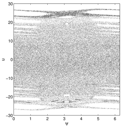
Figure 2:

References

- (1) F.D. Tappert, in Wave Propagation and Underwater Acoustics , edited by J.B. Keller and J.S. Papadakis, Springer-Verlag, Berlin 1977, p. 224.
- (2) F.B. Jensen, W.A. Kuperman, M.B. Porter, and H. Schmidt, Computational Ocean Acoustics, AIP, Woodbury, NY 1994.
- (3) A.L. Virovlyansky and G.M. Zaslavsky, Chaos 10 (2000) 211.
- (4) W. Munk and C. Wunsch, Deep–Sea Res. 26 (1979) 123.
- (5) The ATOC Consortium, Science 1326 (1988).
- (6) M.G. Brown , F.D. Tappert, and G. Goni, Wave Motion 14 (1991) 93.
- (7) D.R. Palmer, M.G.Brown, F.D. Tappert, and M.F. Bezdek, Geophys. Res. Lett. 15 (1988) 569.
- (8) K.B. Smith, M.G. Brown, and F.D. Tappert, J. Acoust. Soc. Am. 91 (1992) 1939, 1950.
- (9) J. Simmen, S.M. Flatte, and G.-Y. Wang, ibid 102 (1997) 239.
- (10) S.S. Abdullaev and G.M. Zaslavsky, Sov. Phys. Usp. 34 (1991) 645.
- (11) B. Sundaram and G.M. Zaslavsky, Chaos 9 (1999) 483.
- (12) I.P. Smirnov, A.L. Virovlyansky, and G.M. Zaslavsky, Phys. Rev. E 64(2001) 036221.
- (13) M.C. Gutzwiller, Chaos in Classical and Quantum Mechanics, Springer-Verlag, New York, 1990.
- (14) G.M. Zaslavsky, Phys. Rep. 80 (1981) 157.
- (15) G.M. Zaslavsky and S.S. Abdullaev, Chaos 7 (1997) 182.
- (16) G.P. Berman and G.M. Zaslavsky, Physica A 91 (1978) 450.
- (17) G.P. Berman and G.M. Zaslavsky, Physica A 111 (1982) 17.
- (18) It should be noted that considerating the higher orders of in the perturbation approach does not change the form of the dispersion relation (4). It leads to the correction of the order of , except for those regions of , where an interaction between different modes (say and ) leads to the avoiding modes crossing, and the corrections to the dispersion law in this case is of the order of .
- (19) A.J. Lichtenberg and M.A. Liberman, Physica D 1 (1980) 291.
- (20) A.J. Lichtenberg and M.A. Liberman, Regular and Stochastic Motion, Springer-Verlag, New York, 1983.
- (21) G. Casati and B.V. Chirikov in Quantum Chaos: Between Order and Disorder, edited by G. Casati and B.V. Chirikov, Cambridge, 1995.
- (22) A. Munier, J.R. Burgan, M. Feix, and E. Fijalkov, J. Math. Phys. 22 (1981) 1219; J.V. Jose and R. Gordery, Phys. Rev. Lett. 56 (1986) 290; C. Scheininger and M. Kleber, Physica D 50 (1990) 391.
- (23) C. Scheininger and M. Kleber, Physica D 50, (1990) 391.
- (24) Semiclassical quantization of the system in the framework of the energy–time canonical variables is not a properly defined task, because the operator is not defined semiclassically iom . Another deficiency is an appearance of the non-physical time (-coordinate in our case) for a wave function. It has been already pointed out grah ; iom that in this case it is impossible to study quantum dynamics. Another question relates to the quasienergy spectrum which is false, as can seen here.
- (25) A. Iomin, S. Fishman, and G.M. Zaslavsky, Semiclassical quantization of maps with a variable time scale, unpublished.
- (26) R. Graham, Europhys. Lett. 7 (1988) 671.
- (27) We restrict ourselves by the expression (24), since an exact analysis is quite cumbersome (see iom ) and is not within the scope of the present analysis.
- (28) E. Jahnke, F. Emde, F. Lösh, Tables of a Higher Functions, New York, McGrow-Hill, 1960.
- (29) L. Rayleigh, Proc. Ray. Soc. A 79 (1907) 399.