Microscopic theory of quantum dot interactions with quantum light: local field effect

Abstract

A theory of both linear and nonlinear electromagnetic response of a single QD exposed to quantum light, accounting the depolarization induced local–field has been developed. Based on the microscopic Hamiltonian accounting for the electron–hole exchange interaction, an effective two–body Hamiltonian has been derived and expressed in terms of the incident electric field, with a separate term describing the QD depolarization. The quantum equations of motion have been formulated and solved with the Hamiltonian for various types of the QD excitation, such as Fock qubit, coherent fields, vacuum state of electromagnetic field and light with arbitrary photonic state distribution. For a QD exposed to coherent light, we predict the appearance of two oscillatory regimes in the Rabi effect separated by the bifurcation. In the first regime, the standard collapse–revivals phenomenon do not reveal itself and the QD population inversion is found to be negative, while in the second one, the collapse–revivals picture is found to be strongly distorted as compared with that predicted by the standard Jaynes-Cummings model. For the case of QD interaction with arbitrary quantum light state in the linear regime, it has been shown that the local field induce a fine structure of the absorbtion spectrum. Instead of a single line with frequency corresponding to which the exciton transition frequency, a duplet is appeared with one component shifted by the amount of the local field coupling parameter. It has been demonstrated the strong light–mater coupling regime arises in the weak-field limit. A physical interpretation of the predicted effects has been proposed.

I Introduction

The strong coupling between condensed matter and quantum light is a core issue of present day quantum optics. Realized by exposing the matter with intense quantum field, it can manifest itself in different quantum systems such as single atoms and ultracold atomic beams Scully , semiconductor heterostructures bimberg_b99 ; Michler_book , Bose–Einstein condensates kasevich , etc. Albeit these systems are of different physical nature, their interaction with quantum light is governed by common rules. In the strong coupling regime, these systems enable the generation of different states of quantum light — single photons lounis_05 , Fock states bratke , Fock qubits, quantum states with arbitrary photon number distribution Law_96 . That constitutes a basis for the quantum information processing Kilin_99 ; zadkov and quantum metrology wheeler . In practice, the strong light–matter coupling regime can be realized in two ways: by combining the matter with a high-Q microcavity or by exposing the matter to a ultrashort intense pump pulse.

To describe the strong coupling between an arbitrary two–level system and quantum light, the Jaynes–Cummings (JC) model is conventionally used Jaynes_Cummings . One of the most fundamental phenomenon predicted within the JC model is the oscillation of the population between levels with the Rabi frequency (Rabi oscillations). However, the standard JC model does not account for a number of physical factors, which, under certain conditions, may significantly influence the Rabi effect. The time–domain modulation of the field–matter coupling constant Law_96 ; yang_04 and interplay between classical driving field and quantized cavity field Law_96 can serve as examples. More advanced JC models involve additional interaction mechanisms and effects, such as dipole–dipole (d–d) interaction lewenstein_94 ; Zhang_94 , exction–phonon coupuling forstner_03 ; dizhu_05 , and self–induced transparency fleischhauer_05 . The d–d interaction between two quantum oscillators leads to radiative coupling of them and, as a result, to exchange by the excited state. That is, Rabi oscillations between these two oscillators occur; see Ref. Dung_02, for a theory and Ref. Unold_05, for the experimental observation in a double quantum dot (QD) system. As a whole, the observation and intensive studying of excitonic Rabi oscillations Unold_05 ; sticvater ; kamada ; htoon ; Zrenner_nature ; sticvater_rep ; mitsumori_05 motivates the extension of the JC–model to incorporate specific interactions inherent to confined exciton in a host.

In the given paper we present a microscopic theory of the interaction of an isolated QD with quantum light for both weak and strong coupling regimes. We incorporate the local field correction into the JC model as an additional physical mechanism influencing the Rabi effect in a QD exposed to quantum light. In particular, the Rabi oscillations are shown to exist even in the limit of a weak incident field.

In the weak coupling regime, the local–field effects in optical properties of QDs have been theoretically investigated in Refs. Schmitt_87, ; Hanewinkel_97, ; Slepyan_99a, ; Maksim_00a, ; Ajiki_02, ; Goupalov_03, ; Slepyan_NATO_03, ; Maksimenko_ENN, ; Maksimenko_HN04, for classical exposing light and in Ref. maxim_pra_02, for quantum light. In the latter case it has been shown that for a QD interacting with Fock qubits the local fields induce a fine structure of the absorption (emission) spectrum: instead of a single line with the frequency corresponding to the exciton transition, a doublet appears with one component shifted to the blue (red). The intensities of components are completely determined by the quantum light statistics. In the limiting cases of classical light and Fock states the doublet is reduced to a singlet shifted in the former case and unshifted in the latter one.

The role of local fields in the excitonic Rabi oscillations in an isolated QD driven by classical excitation was investigated in Ref. magyar04, . Two different oscillatory regimes separated by the bifurcation have been predicted to exist. The Rabi oscillations were predicted to be non-isochronous and arising in the weak excitation regime. Both peculiarities have been experimentally observed by Mitsumori et al. in Ref. mitsumori_05, where the Rabi oscillations of excitons localized to quantum islands in a single quantum well were investigated.

There exist several different physical interpretations of local field in QDs and, correspondingly, different ways of its theoretical description. The first model (scheme A in the terminology of Ref. Ajiki_02, ) exploits the standard electrodynamical picture: by virtue of external field screening by charges induced on the QD surface (the quasistatic Coulomb electron–hole interactions) a depolarization field is formed differentiating the local (acting) field in the QD and external incident field. In this model the total electromagnetic field is not pure transverse. Alternatively, only transverse component is attributed to the electromagnetic field, while the longitudinal component is accounted for through the exchange electron–hole interactions (scheme B accordingly Ref. Ajiki_02, ). Both approaches are physically equivalent and lead to identical results.

In the present paper we build the analysis on the general microscopic quantum electrodynamical (QED) approach where the local field correction originates from the exchange by virtual vacuum photons between electrons and holes forming the exciton and thus is a manifestation of the dipole–dipole (d–d) interaction between electrons and holes (the dynamical Coulomb interaction) lewenstein_94 ; Zhang_94 . The approach allows us to overcome a number of principal difficulties related to the field quantization in QDs ref01 . In the analysis, approximate solution of the many–body problem is built on the Hartree–Fock–Bogoliubov self–consistent field concept lewenstein_94 . The self-consistent technique leads to a separate term in the effective Hamiltonian responsible for the interaction of operators and average values of physical quantities. Due to this term the quantum mechanical equations of motion become nonlinear and require numerical integration.

The paper is arranged as follows. In Sect. II we develop theoretical model describing the QD–quantum light interaction. We formulate a model Hamiltonian with the separate term accounting for the local field correction and corresponding equations of motion. In Sect. III we analyze the manifestation of local fields in the motion of the QD exciton in the absence of external field. In Sec. IV we investigate the QD interaction with arbitrary state of quantum light in the weak driving field regime. Sect. V is devoted to the theoretical analysis of local field influence on the Rabi oscillations in the QD exposed to coherent states of light and Fock qubits. A discussion of the results obtained is presented in Sect. VI and concluding remarks are given in Sect. VII.

II Quantum Dot – quantum light Interaction: theoretical model

II.1 Interaction Hamiltonian

In this section we formulate the interaction Hamiltonian for a QD exposed to quantized field accounting for the local–field correction. Later on we exploit the Hamiltonian for the derivation of equations of motions describing dynamical properties of this system.

As aforementioned, the local field in QD differs from the incident one due to the d–d electrons–holes interaction. A general formalism accounting for the d–d interactions in atomic many–body systems exposed to photons has been developed in Refs. lewenstein_94, ; Zhang_94, as applied to nonlinear optics of Bose–Einstein condensates lewenstein_94 ; Zhang_94 . We extend this formalism to the case of the QD exciton driven by quantized light.

Consider an isolated QD exposed to quantized electromagnetic field. The electron–hole pairs in QD are assumed to be strongly confined; thus we neglect the static Coulomb interaction between electrons and holes. We decompose the operator of the total electromagnetic field into two components. The first one, $\widehat{\bm{\mathcal{E}}}_{\mathrm{v}}$, represents a set of modes that do not contain real photons. The second component, $\widehat{\bm{\mathcal{E}}}_{\mathrm{0}}$, represents the set of modes emitted by the external source of light (real photons). Such a decomposition as well as the subsequent separate consideration of the field components is analogous to the Heisenberg–Langvein approach in the quantum theory of damping, see Ref. Scully, . The total Hamiltonian of the system ”QD+electromagnetic field” is then represented as

$$\widehat{{\cal H}}=\widehat{{\cal H}}_{\mathrm{0}}+\widehat{{\cal H}}_{\mathrm{ph}}+\widehat{{\cal H}}_{\mathrm{vac}}+\widehat{{\cal H}}_{\mathrm{I0}}+\widehat{{\cal H}}_{\mathrm{Iv}}\,,$$ (1)

where $\widehat{{\cal H}}_{\mathrm{0,ph,vac}}$ are the Hamiltonians of the QD free charge carriers, the incident photons and the virtual vacuum photons, respectively. The terms $\widehat{{\cal H}}_{\mathrm{I0,Iv}}$ describe the interaction of electron–hole pair with incident quantum field $\widehat{\bm{\mathcal{E}}}_{\mathrm{0}}$ and with vacuum field $\widehat{\bm{\mathcal{E}}}_{\mathrm{v}}$, respectively. In the dipole approximation these Hamiltonians are given by

$$\widehat{{\cal H}}_{\mathrm{I0,Iv}}=-\frac{1}{2}\int_{V}(\widehat{\bm{\mathcal{P}}}\widehat{\bm{\mathcal{E}}}_{\mathrm{0,v}}+\widehat{\bm{\mathcal{E}}}_{\mathrm{0,v}}\widehat{\bm{\mathcal{P}}})\,d^{3}\mathbf{r}\,$$ (2)

where $V$ is the QD volume and $\widehat{\bm{\mathcal{P}}}(\bm{r},t)$ is the QD polarization operator. The Hamiltonian $\widehat{{\cal H}}_{\mathrm{vac}}$ is as follows

$$\widehat{{\cal H}}_{\mathrm{vac}}=\sum_{k\lambda}\hbar\omega_{k}\hat{v}^{\dagger}_{k\lambda}\hat{v}_{k\lambda}\,,$$ (3)

where $\hat{v}^{\dagger}_{k\lambda}$ and $\hat{v}_{k\lambda}$ are the creation and annihilation operators of vacuum photons, $k$ is the mode index, indexes $\lambda=1,2$ denote the field polarization. The operator of vacuum electromagnetic field $\widehat{\bm{\mathcal{E}}}_{\mathrm{v}}$ is determined as

$$\widehat{\bm{\mathcal{E}}}_{\mathrm{v}}=i\sum_{k\lambda}\sqrt{\frac{2\pi\hbar\omega_{k}}{\Omega}}{\,}\textbf{e}_{k\lambda}(\hat{v}_{k\lambda}{e}^{i\textbf{kr}}-\hat{v}^{\dagger}_{k\lambda}{e}^{-i\mathbf{kr}})\,,$$ (4)

where $\Omega$ is the normalization volume and $\mathbf{e}_{k\lambda}$ is the polarization unit vector.

As a first step in the development of our theory we eliminate from the consideration the exchange interactions and proceed to the direct interactions. For that purpose, we exclude the vacuum photon operators $\hat{v}_{k\lambda}$ and $\hat{v}^{\dagger}_{k\lambda}$ expressing them (and corresponding Hamiltonians $\widehat{{\cal H}}_{\mathrm{vac}}$ and $\widehat{{\cal H}}_{\mathrm{Iv}}$) in terms of the polarization operator $\widehat{\bm{\mathcal{P}}}$. Recalling the Heisenberg equation $i\hbar\partial{\hat{v}_{k\lambda}}/\partial{t}=-\left[\widehat{{\cal H}},\hat{v}_{k\lambda}\right]$, the expression as follows can be obtained,

$$\frac{\partial{}\hat{v}_{k\lambda}}{\partial{t}}=-i\omega_{k}\hat{v}_{k\lambda}+\widehat{F}_{k\lambda}(t)\,,$$ (5)

where $\widehat{F}_{k\lambda}(t)=\sqrt{2\pi\omega_{k}/\hbar{\Omega}}\int\limits_{V}\widehat{\bm{\mathcal{P}}}(\textbf{r}^{\prime},t)\textbf{e}_{k\lambda}e^{i\textbf{kr}}d^{3}{\textbf{r}^{\prime}}$. Solution of Eq. (5) is given by

$$\hat{v}_{k\lambda}(t)=\hat{v}_{k\lambda}(-\infty)e^{-i\omega_{k}t}+\int\limits_{-\infty}^{t}\!\widehat{F}_{k\lambda}(\tau)e^{-i\omega_{k}(t-\tau)}d\tau\,$$ (6)

with the first term describing the free evolution of the reservoir modes (quantum noise) and the second one responsible for the exchange interactions. Further we neglect the first term in (6) leaving the quantum noise beyond the consideration. Inserting then this equation into (4) and the resulting expression – into Hamiltonian (2), after some algebra we arrive at

$$\widehat{{\cal H}}_{\mathrm{Iv}}=-\sum_{k}\frac{2\pi{i}\omega_{k}}{\Omega}\int\limits_{-\infty}^{t}\!\!\int\limits_{V}\!\!\int\limits_{V}\widehat{{\mathcal{P}}}_{\alpha}(\textbf{r},t)\widehat{{\mathcal{P}}}_{\beta}(\textbf{r}^{\prime},\tau)~{}~{}~{}~{}~{}~{}~{}~{}$$ (7)

$$\rule{0.0pt}{17.22217pt}\sum_{\lambda}{\bf\rm e}^{(\alpha)}_{k\lambda}{\bf\rm e}^{(\beta)}_{k\lambda}e^{i\rm{\bf k}({\bf r}-{\bf r}^{\prime})}e^{i\omega_{k}(\tau-t)}d\tau{}d^{3}{\bf r}\,d^{3}{\bf r}^{\prime}+\rm{H.c.}\,,$$ (8)

where indexes $\alpha$, $\beta$ mark Cartesian projections of vectors. The summation over repetitive indexes is assumed. Using the relationship Scully

$$\sum_{\lambda}{\rm e}^{(\alpha)}_{k\lambda}{\rm e}^{(\beta)}_{k\lambda} = \delta_{\alpha\beta}-\frac{k_{\alpha}k_{\beta}}{k^{2}}$$

$$= \frac{1}{k^{2}}\left(\frac{\partial^{2}}{\partial{x_{\alpha}}\partial{x_{\beta}}}-\delta_{\alpha\beta}\frac{1}{c^{2}}\frac{\partial^{2}}{\partial{t^{2}}}\right)\,,$$

we proceed to the limit $\Omega\rightarrow\infty$ in (8). That corresponds to the replacement

$$\sum_{k}[\cdot]\rightarrow\frac{\Omega}{(2\pi)^{3}}\int{[\cdot]}d^{3}\textbf{k}\,.$$

Then, utilizing the Markov property of the polarization operator, $\widehat{{\mathcal{P}}}_{\alpha}(\textbf{r},t)\simeq\widehat{{\mathcal{P}}}_{\alpha}(\textbf{r},0)$ [Zhang_94, ], the Hamiltonian (8) is reduced to

$$\widehat{{\cal H}}_{\mathrm{Iv}} = -4\pi\int\limits_{0}^{\infty}\!\!\int\limits_{V}\!\!\int\limits_{V}\left(\frac{\partial^{2}}{\partial{x_{\alpha}}\partial{x_{\beta}}}-\delta_{\alpha\beta}\frac{1}{c^{2}}\frac{\partial^{2}}{\partial{{t^{\prime}}^{2}}}\right)~{}~{}~{}~{}$$ (10)

$$\times G^{(0)}(\textbf{r}-\textbf{r}^{\prime},t^{\prime})\widehat{{\mathcal{P}}}_{\alpha}(\textbf{r},t)\widehat{{\mathcal{P}}}_{\beta}(\textbf{r}^{\prime},t)d{t^{\prime}}d^{3}\textbf{r}d^{3}\textbf{r}^{\prime}\,,$$ (11)

where

$$G^{(0)}({\bf r},t) = \frac{ic^{2}}{2(2\pi)^{3}}\int\frac{e^{i{\bf kr}}}{\omega_{k}}\left(e^{-i\omega_{k}t}-e^{i\omega_{k}t}\right)d^{3}{\bf k}$$ (12)

$$= \frac{1}{4\pi|{\bf r}|}\left[\delta\left(\frac{|{\bf r}|}{c}-t\right)-\delta\left(\frac{|{\bf r}|}{c}+t\right)\right]\,,$$ (13)

is the free-space Green function beresteckij and $\delta(\dots)$ is the Dirac delta–function. Evaluation of $\widehat{{\cal H}}_{\mathrm{vac}}$ in (3) is carried out analogously and gives $\widehat{{\cal H}}_{\mathrm{vac}}=-\widehat{{\cal H}}_{\mathrm{Iv}}/2$.

As the next step, we adopt the quasi–static approximation, which utilizes the property of QD to be electrically small. The approximation implies the limit transition $c\rightarrow\infty$ and the neglect the terms $\sim\partial^{2}/\partial{t^{\prime}}^{2}$ in Hamiltonian (10). Then, the Hamiltonians $\widehat{{\cal H}}_{\mathrm{vac}}$ and $\widehat{{\cal H}}_{\mathrm{Iv}}$ are represented by the sum as follows

$$\Delta{\widehat{{\cal H}}} = \widehat{{\cal H}}_{\mathrm{vac}}+\widehat{{\cal H}}_{\mathrm{Iv}}$$ (14)

$$= -\frac{1}{2}\int\limits_{V}\!\!\int\limits_{V}\!\!\widehat{\bm{\mathcal{P}}}(\mathbf{r})\underline{G}(\mathbf{r}-\mathbf{r}^{\prime})\widehat{\bm{\mathcal{P}}}(\mathbf{r}^{\prime})\,d^{3}\mathbf{r}\,d^{3}\mathbf{r}^{\prime}\,,$$ (15)

where

$$\underline{G}({\bf r}-\mathbf{r}^{\prime})=\nabla_{\mathbf{r}}\otimes\nabla_{\mathbf{r}}\left(\frac{1}{|\mathbf{r}-\mathbf{r}^{\prime}|}\right)$$ (16)

is the free space Green tensor; $\nabla_{\mathbf{r}}\otimes\nabla_{\mathbf{r}}$ is the operator dyadic acting on variables $\mathbf{r}$. In the quasi–static approximation we neglect the line broadening due to the dephasing and the spontaneous emission. The latter effect can be introduced in the model by retaining terms $O(1/c)$ in the the quasi–static approximation.

In the preceding analysis we have suggested that the exchange by virtual photons of all modes occurs between all allowed dipole transitions. That is, on that stage the problem was stated as a quantum–mechanical many–body problem. The analysis can be significantly simplified if we restrict ourselves to the two–level approximation assuming the exciton transition frequency to be resonant with the acting field carrier frequency and utilize the self–consistent field model. The self–consistent field is introduced by means of the Hartree–Fock–Bogoliubov approximation hartree_rigourus , which implies the linearization of Hamiltonian (14) by the substitution

$$\widehat{{\bm{\mathcal{P}}}}({\bf r})\widehat{{\bm{\mathcal{P}}}}({\bf r}^{\prime})\rightarrow\widehat{{\bm{\mathcal{P}}}}({\bf r})\langle\widehat{{\bm{\mathcal{P}}}}({\bf r}^{\prime})\rangle+\langle\widehat{{\bm{\mathcal{P}}}}({\bf r})\rangle\widehat{{\bm{\mathcal{P}}}}({\bf r}^{\prime})\,.$$ (17)

The polarization operator of two-level system is given by Cho_b03

$$\widehat{{\bm{\mathcal{P}}}}({\bf r})=|\zeta({\bf r})|^{2}({\bm{\mu}}\hat{\sigma}_{+}+{\bm{\mu}}^{*}\hat{\sigma}_{-})\,,$$ (18)

where $\hat{\sigma}_{\pm}$ are the Pauli pseudospin operators and $\zeta({\bf r})$ is the wavefunction of the electron–hole pair. In the strong confinement regime this function is assumed to be turns out to be the same both in excited and ground states Chow_b99 ; haug_b94 .

In the two–level approximation, the Hamiltonian of the carriers motion is represented as

$$\widehat{{\cal H}}_{0}=\varepsilon_{\mathrm{e}}\hat{a}_{\mathrm{e}}^{{\dagger}}\hat{a}_{\mathrm{e}}+\varepsilon_{\mathrm{g}}\hat{a}_{\mathrm{g}}^{{\dagger}}\hat{a}_{\mathrm{g}}\,,$$ (19)

where $\varepsilon_{\mathrm{g},\mathrm{e}}$ and $\hat{a}_{\mathrm{g,e}}^{{\dagger}}$/$\hat{a}_{\mathrm{{g,e}}}$ are the energy eigenvalues and creation/annihilation operators of the exciton; indices $\mathrm{e}$ and $\mathrm{g}$ correspond to the excitonic excited and ground states, respectively. The acting field operator is expressed by the relation (4) after the substitutions $\hat{v}_{k\lambda}\rightarrow{}\hat{c}_{q}(t)$ and $\hat{v}^{\dagger}_{k\lambda}\rightarrow{}\hat{c}^{\dagger}_{q}(t)$; $\hat{c}^{\dagger}_{q}(t)/\hat{c}_{q}$ are the creation/annihilation operators of the incident (real) photons (the polarization index $\lambda$ is included in the mode number $q$). Formally, the relation (6) is fulfilled for operators $\hat{c}_{q}(t)$ and $\hat{c}^{\dagger}_{q}(t)$ too, and the first term describes the evolution of real photons. However, since the exchange interaction is included into the vacuum field component, in the case of real photons the second term in relation (6) disappears. Then, the Hamiltonian $\widehat{{\cal H}}_{\rm{ph}}$ is given by the relation (3) after the substitution $\hat{v}_{k\lambda}\rightarrow{}\hat{c}_{q}(-\infty)$ and $\hat{v}^{\dagger}_{k\lambda}\rightarrow\hat{c}^{\dagger}_{q}(-\infty)$. For shortness, we denote $\hat{c}_{q}(-\infty)=\hat{c}_{q}$ and $\hat{c}^{\dagger}_{q}(-\infty)=\hat{c}^{\dagger}_{q}$ .

Note that nonresonant transitions can be approximately accounted through a real–valued frequency–independent background dielectric function $\epsilon_{h}$. Assuming $\epsilon_{h}$ to be equal to dielectric function of surrounding medium, we put further $\epsilon_{h}=1$ without loss of generality. Substitutions in final expressions $c\to c/\sqrt{\epsilon_{h}}$ and ${\bm{\mu}}\to{\bm{\mu}}/\sqrt{\epsilon_{h}}$ for the speed of light and the electron-hole pair dipole moment, respectively, will restore the case $\epsilon_{h}\neq 1$.

As a next step we introduce the rotating wave approximation Scully , i.e., we neglect in (10) the terms that are responsible for the simultaneous creation/annihilation of exciton-exciton and exciton-photon pairs. Then, using expressions (2), (3) and (10)–(18), after some algebra we derive the effective two–particle Hamiltonian

$$\widehat{{\cal H}}_{\mathrm{eff}} = \widehat{{\cal H}}_{\mathrm{0}}+\widehat{{\cal H}}_{\mathrm{ph}}+\widehat{{\cal H}}_{\mathrm{I0}}+\Delta{\widehat{{\cal H}}}\,,$$ (20)

where

$$\widehat{{\cal H}}_{\mathrm{I0}} = \hbar\sum\limits_{q}(g_{q}\hat{\sigma}_{+}\hat{c}_{q}+g^{*}_{q}\hat{\sigma}_{-}\hat{c}^{\dagger}_{q})$$ (21)

and

$$\Delta\widehat{{\cal H}} = \frac{4\pi}{V}\bm{\mu}(\tilde{\underline{N}}\bm{\mu})(\hat{\sigma}_{-}\langle\hat{\sigma}_{+}\rangle+\hat{\sigma}_{+}\langle\hat{\sigma}_{-}\rangle)\,.$$ (22)

where $g_{q}=-i\bm{\mu}{\bf e}_{q}\sqrt{2\pi\omega_{k}/\hbar\Omega}\exp(i{\bf kr}_{c})$ is the coupling factor for photons and carriers in the QD and ${\bf r}_{c}$ is the radius–vector of the QD geometrical center. The depolarization tensor is given by

$$\tilde{\underline{N}}=-\frac{V}{4\pi}\int\limits_{V}\!\!\int\limits_{V}|\xi(\mathbf{r})|^{2}\,|{\xi}(\mathbf{r}^{\prime})|^{2}\underline{G}({\bf r}-\mathbf{r}^{\prime})d^{3}\mathbf{r}\,d^{3}\mathbf{r}^{\prime}\,.$$ (23)

Noted that the resulting Hamiltonian (20) coincides with that obtained in Ref. maxim_pra_02, in independent way.

II.2 Equations of motions

Let $|\widetilde{\psi}(t)\rangle$ be a wavefunction of a QD interacting with quantum light. In the interaction representation the system is described by the Schrödinger equation

$$i\hbar\frac{\partial|\psi\rangle}{\partial t}=\widehat{{\cal H}}_{\rm{int}}|\psi\rangle\,,$$ (24)

with $|\psi(t)\rangle=\exp[i(\widehat{{\cal H}}_{\rm{0}}+\widehat{{\cal H}}_{\rm{ph}})t/\hbar]|\widetilde{\psi}(t)\rangle$ and $\widehat{{\cal H}}_{\rm{int}}=\exp[i(\widehat{{\cal H}}_{\rm{0}}+\widehat{{\cal H}}_{\rm{ph}})t/\hbar](\widehat{{\cal H}}_{\mathrm{I0}}+\Delta\widehat{{\cal H}})\exp[-(i\widehat{{\cal H}}_{0}+\widehat{{\cal H}}_{\rm{ph}})t/\hbar]$. We represent the wavefunction $|\psi(t)\rangle$ by the sum as follows

$$|\psi(t)\rangle=\sum_{\{n_{k}\}\geq{0}}\left[A_{\{n_{k}\}}(t)|e\rangle+B_{\{n_{k}\}}(t)|g\rangle\right]|\{n_{k}\}\rangle\,,$$ (25)

where $A_{\{n_{k}\}}(t)$ and $B_{\{n_{k}\}}(t)$ are coefficients to be found, $|\{n_{k}\}\rangle$ denotes the multimode field state with $n$ photons in $k$ mode; $|\{0_{k}\rangle\}$ is the wavefunction of the vacuum state of electromagnetic field; $|e\rangle$ and $|g\rangle$ are the wavefunctions of the QD ground and excited states, respectively. By inserting the relation (25) into the Schrödinger equation (24), after some manipulations we arrive at the system of equations of motion

$$i\frac{dA_{\{m_{l}\}}}{dt} = \Delta\omega B_{\{m_{l}\}}\sum\limits_{\{n_{q}\}}A_{\{n_{q}\}}B_{\{n_{q}\}}^{*}$$ (26)

$$+ \sum_{q}g_{q}\sqrt{m_{q}+1}B_{\{m_{l}+\delta_{lq}\}}e^{i(\omega_{0}-\omega_{q})t}\,,$$ (27)

$$i\frac{dB_{\{m_{l}\}}}{dt} = \Delta\omega A_{\{m_{l}\}}\sum\limits_{\{n_{q}\}}A_{\{n_{q}\}}^{*}B_{\{n_{q}\}}$$ (28)

$$+ \sum_{q}g^{*}_{q}\sqrt{m_{q}}A_{\{m_{l}-\delta_{lq}\}}e^{-i(\omega_{0}-\omega_{q})t}\,,~{}~{}$$

with

$$\Delta\omega=\frac{4\pi}{\hbar{}V}{\bm{\mu}}(\widetilde{{\underline{N}}}{\bm{\mu}})\,,$$ (29)

as the local–field induced depolarization shift Slepyan_99a ; maxim_pra_02 . Here $\omega_{0}=(\varepsilon_{\mathrm{e}}-\varepsilon_{\mathrm{g}})/\hbar$ is exciton transition frequency. It can easily be shown that system (26) satisfies the conservation law

$$\frac{d}{dt}\sum_{\{n_{k}\}}(|{A}_{\{n_{k}\}}|^{2}+|{B}_{\{n_{k}\}}|^{2})=0\,.$$ (30)

The system (26) allows analyzing the interaction between QD and electromagnetic field of an arbitrary spatial configuration and arbitrary polarization. Letting the coefficients $g_{q}(t)$ to be adiabatically slow–varying functions we can apply (26) to QDs exposed to electromagnetic pulse.

II.3 Single–mode approximation

Among different physical situations described by Eqs. (26) the single-mode excitation is of special interest. Indeed, such a case corresponds, for instance, to the light –QD interaction in a microcavity with a particular mode resonant with the QD exciton. Owing to the high Q-factor, the strong light–QD coupling regime is feasible in microcavity providing numerous potential applications of such systems Scully ; Michler_book .

For the case of a spherical QD interacting with single–mode light, only the components $|\{n_{k}\}\rangle=|0_{1},0_{2},\dots{n_{q}}\dots{0_{k}}\dots\rangle=|n_{q}\rangle$ with $q$ as the number of interacting mode are accounted for in the wavefunction (25). Then, omitting for shortness the mode number, the system (28) is reduced to

$$i\frac{d{A}_{n}}{dt} = \Delta\omega{B}_{n}\sum\limits_{m}{A}_{m}{B}_{m}^{*}$$ (31)

$$+ g\sqrt{n+1}{B}_{n+1}e^{i(\omega_{0}-\omega)t}\,,$$ (32)

$$\rule{0.0pt}{17.22217pt}i\frac{d{B}_{n+1}}{dt} = \Delta\omega{A}_{n+1}\sum\limits_{m}{A}_{m}^{*}{B}_{m}$$ (33)

$$+ g^{*}\sqrt{n+1}{A}_{n}e^{-i(\omega_{0}-\omega)t}\,.~{}~{}$$

Note that the conservation law (30) holds true for Eqs. (32) with the substitution $\{n_{k}\}\rightarrow{n}$. Equations (26) and (32) govern the time evolution of the QD driven by quantum light.

III Free motion

The free motion regime implies neglect the QD–electromagnetic field interaction and thus imposes the condition $g=0$ on Eqs. (31). Wavefunction of the noninteracting QD and electromagnetic field is factorized thus allowing analytical solution of (31) in the form of

$$\displaystyle A_{n}(t)=C_{n}A(t)\,,\qquad\displaystyle B_{n}(t)=C_{n}B(t)\,,$$

where $C_{n}$ are arbitrary constants satisfying the normalization condition $\sum_{n}|C_{n}|^{2}=1$. In that case the system (31) is reduced to the exactly integrable form

$$\displaystyle i\frac{dA}{dt}=\Delta\omega A|B|^{2}\,,\qquad\displaystyle i\frac{dB}{dt}=\Delta\omega B|A|^{2}\,,$$ (34)

and its solution is given by

$$\displaystyle A(t)=a_{0}e^{-i\Delta\omega|b_{0}|^{2}t}\,,\quad\displaystyle B(t)=b_{0}e^{-i\Delta\omega|a_{0}|^{2}t}\,.$$ (35)

Here $a_{0}$ and $b_{0}$ are arbitrary constants satisfying the condition $|a_{0}|^{2}+|b_{0}|^{2}=1$. This solution describes a correlated motion of the electron-hole pair resulted from the local field–induced self-polarization of the QD. Thus, a quasi–particle with the wavefunction

$$|\widetilde{\psi}(t)\rangle=A(t){e^{-i\omega_{e}t}}|e\rangle+B(t){e^{-i\omega_{g}t}}|g\rangle\,,$$ (36)

appears in the QD. It can easily be shown that the state (36) satisfies the energy and probability conservation laws. The inversion, which is defined as the difference between the excited–state and the ground-state populations of the QD exciton, for the wavefunction (36) remains constant in time: $w=|A(t)|^{2}-|B(t)|^{2}\equiv|a_{0}|^{2}-|b_{0}|^{2}$, whereas this state is generally non-stationary. The quasi–particle lifetime, which is not included in our model, can be estimated by $\tau_{\mathrm{sp}}\sim 1/\Gamma_{\mathrm{sp}}$, where $\Gamma_{\mathrm{sp}}$ is the QD–exciton spontaneous decay rate. For realistic QDs $\Delta\omega\gg 1/\Gamma_{\mathrm{sp}}$ [maxim_pra_02, ]. Consequently, the state $|\widetilde{\psi}(t)\rangle$ can be treated as stationary within the range $1/\Delta\omega\ll{}t\ll 1/\Gamma_{\mathrm{sp}}$.

The macroscopic polarization of the QD is described by

$$\langle{\widehat{\bm{\mathcal{P}}}}\rangle=\langle\psi|\widehat{\bm{\mathcal{P}}}|\psi\rangle=\frac{1}{V}{\bm{\mu}}a_{0}b^{*}_{0}e^{-i(\omega_{0}-\delta^{\prime})t}+\rm{c.c.}\,,$$ (37)

where the parameter $\delta^{\prime}={w}\Delta\omega$ plays the role of the self–induced detuning, which depends on the state occupied by the exciton and on the depolarization shift. Thus, as follows from (37), the local field–induced depolarization shift ($\Delta\omega\neq 0$) dictates the non-isochronism of the polarization oscillations, i.e. the dependence of the oscillations frequency on its amplitude. This mechanism also influences the Rabi oscillations in the system: the smaller $\delta^{\prime}$ the larger Rabi oscillations amplitude; such a behavior was observed experimentally in Ref. mitsumori_05, .

Since the inversion $w$ lies within the range $-1\leq{w}\leq{1}$, the frequency $\omega_{p}$ of polarization oscillations in (37) may vary in the limits $\omega_{0}-\Delta\omega\leq\omega_{p}\leq\omega_{0}+\Delta\omega$. On the contrary, when $\Delta\omega=0$ the polarization oscillates with the fixed frequency $\omega_{0}$. At first glance, it seems that the discrete level is transformed into $2\Delta\omega$ band. However this is not the case. Indeed, the concept of the band structure corresponds to linear systems where any arbitrary state is a superposition of eigenmodes with different frequencies. As different from that, the electron–hole correlation arises from the nonlinear motion of the particles in a self-consistent field. Consequently, in the presence of light–QD interaction ($g\neq 0$), the exciton motion can not be described by a simple superposition of different partial solutions like (35), but has significantly more complicate behavior. In particular, in the strong coupling regime there exist two oscillatory regimes with drastically different characteristics separated by the bifurcation, see Sec. V.

IV The weak–field approximation

Consider a ground–state QD be exposed to an arbitrary state of quantum light $\sum_{m_{l}}\beta_{\{m_{l}\}}|\{m_{l}\}\rangle$, where $\beta_{\{m_{l}\}}$ are arbitrary complex–valued coefficients satisfying the condition $\sum_{\{m_{l}\}}|\beta_{\{m_{l}\}}|^{2}=1$. Then, the initial conditions for Eqs. (26) are given by

$$A_{\{m_{l}\}}(0)=0,\,\,\,B_{\{m_{l}\}}(0)=\beta_{\{m_{l}\}}\,.$$ (38)

In the linear regime with respect to the electromagnetic field which realized when $g_{q}\rightarrow 0$ we can assume $B_{\{m_{l}\}}(t)\approx{}\beta_{\{m_{l}\}}={\rm{const}}$, i.e. the analysis is restricted to the time interval much less than the relaxation time of the given exciton state. Then, the system (28) is reduced to

$$\frac{dA_{\{m_{l}\}}}{dt} = -i\Delta\omega\sum\limits_{\{n_{q}\}}A_{\{n_{q}\}}\beta_{\{m_{l}\}}\beta_{\{n_{q}\}}^{*}$$ (39)

$$- \sum\limits_{q}g_{q}\sqrt{m_{q}+1}\beta_{\{m_{l}+\delta_{lq}\}}e^{i(\omega_{0}-\omega_{q})t}\,.$$ (40)

For further analysis we rewrite (40) in more convenient matrix notation:

$$\frac{d{\bf a}(t)}{dt}=-i\Delta\omega{\bm{\rho}}{\bf a}(t)-{\bf f}(t)\,,$$ (41)

where ${\bf a}(t)$, ${\bf f}(t)=\sum_{q}{\bf f}_{q}{e^{i(\omega_{0}-\omega_{q})t}}$ and ${\bm{\beta}}$ are the columnar matrices (vectors) and ${\bf a}(t)=(A_{\{m_{l}\}})$. Vectors ${\bf f}_{q}$ and ${\bm{\beta}}$ are defined analogously through the elements $f^{\{m_{l}\}}_{q}=ig_{q}\sqrt{m_{q}+1}\beta_{\{m_{l}+\delta_{ql}\}}$ and $\beta_{\{m_{l}\}}$, respectively; $\delta_{ql}$ is the Kroneker symbol. The quantity ${\bm{\rho}}={\bm{\beta}}{\bm{\beta}}^{{\dagger}}$ is the density matrix of quantum light interacting with the QD. This matrix corresponds to the pure state of electromagnetic field and satisfies the conditions ${\bm{\rho}}^{n}={\bm{\rho}}$ ($n\geq 1$) and ${\bm{\rho}}^{0}=\mathbf{I}$ (where $\mathbf{I}$ is the unit matrix). Integration of (41) imposed by initial conditions (38) allows us to find the analytical solution

$${\bf a}(t)=-\int\limits_{0}^{t}{e^{-i{\bm{\rho}}\Delta\omega(t-t^{\prime})}{\bf f}(t^{\prime})dt^{\prime}}\,.$$ (42)

Using the truncated Taylor expansion ref02

$$e^{-i{\bm{\rho}}\Delta\omega(t-t^{\prime})}=\mathbf{I}-{\bm{\rho}}(1-e^{-i\Delta\omega(t-t^{\prime})})\,,$$

after some standard manipulations we obtain

$${\bf a}(t) = -i\sum\limits_{q}\left[({\bm{\rho}}-\mathbf{I}){\bf f}_{q}\frac{1-e^{i(\omega_{0}-\omega_{q})t}}{\omega_{0}-\omega_{q}-i0}\right.$$ (43)

$$- \left.\bm{\rho}{{\bf f}_{q}}e^{-i\Delta\omega{t}}\frac{(1-e^{i(\omega_{0}-\omega_{q}+\Delta\omega)t})}{\omega_{0}-\omega_{q}+\Delta\omega-i0}\right]\,.$$ (44)

This expression describes the interaction between the QD and an arbitrary state of quantum field in the weak–field limit.

Now let us calculate the QD effective scattering cross-section defined by

$$\sigma(\infty)=\lim_{t\rightarrow{\infty}}\frac{d}{dt}|{\bf a}(t)|^{2}\,.$$ (45)

Substituting (44) into (45), after some algebra we arrive at

$$\sigma(\infty)=2\pi\sum_{\nu=1,2}\sum_{q}|{\bf C}_{\nu{q}}|^{2}\delta{(\omega_{\nu}-\omega_{q})}\,,$$ (46)

where ${\bf C}_{1q}=(\bm{\rho}-\mathbf{I}){\bf f}_{q}$ and ${\bf C}_{2q}=\bm{\rho}\,{\bf f}_{q}$, $\omega_{1}=\omega_{0}$. The equation obtained demonstrates a fine structure of the absorption in a QD exposed to quantum light with arbitrary statistics. Instead of a single line with the exciton transition frequency $\omega_{1}=\omega_{0}$, a doublet appears with one component shifted to the blue: $\omega_{2}=\omega_{0}+\Delta\omega$. The intensities of components are completely determined by the quantum light statistics. The same peculiarity has been revealed in Ref. maxim_pra_02, in a particular case of a QD exposed to the single–mode Fock qubit. Obviously, this result directly follows from (46) if we retain in this equation only terms corresponding the mode considered. The single–mode Fock qubit is a superposition of two arbitrary Fock states with fixed number of photons and is described by the wavefunction (the mode index $q$ is omitted)

$$|\psi\rangle=\beta_{N}|N\rangle+\beta_{N+1}|N+1\rangle\,.$$ (47)

Consequently, at $N\geq 1$ the nonzero components of the vector ${\bf f}_{q}$ are $f^{(N-1)}=ig\sqrt{N}\beta_{N}$ and $f^{(N)}=ig\sqrt{N+1}\beta_{N+1}$ . It can easily be found that in that case Eq. (46) is reduced to Eq. (61) from Ref. maxim_pra_02, . In the case $N=0$ the only nonzero component $f^{(0)}=ig\beta_{1}$ survives in (46) thus reducing this equation to Eq. (67) from Ref. maxim_pra_02, . For the single Fock state $|\psi\rangle=|N\rangle$ and we obtain ${\bf C}_{2}=0$, i.e., in agreement with Ref. maxim_pra_02, , only shifted spectral line is presented in the effective cross–section.

For the QD exposed to coherent states the recurrent formula $\beta_{n+1}=\sqrt{\langle{n}\rangle/(n+1)}\beta_{n}$ can easily be obtained, where $\langle{n}\rangle$ stands for the photon number mean value. Using this formula the relation $\bm{\rho}{\bf f}={\bf f}$ can be obtained, which gives ${\bf C}_{1}=0$. Thus, for this case only shifted line in the effective cross section is manifested. Analogous result has been reported in maxim_pra_02, for a QD driven by classical electromagnetic field. Such a coincidence can be treated as the manifestation of well known concept: among a variety of quantum states of light the coherent states are most close to classical electromagnetic field.

V The quantum light–QD strong coupling regime. Rabi oscillations

In the case when the coupling constant is comparable in value with the exciton decay rate, the linearization with respect to electromagnetic field utilized in the previous section is no longer admissible. The strong coupling regime can be realized by combining the QD with a high-Q microcavity and one of its manifestation is the Rabi oscillations of the levels population in a two–level system exposed to a strong electromagnetic wave. In this section we utilize the system of equations (31) for investigation of the interaction between QD and single–mode quantum light. The incident field statistics is exemplified by coherent states and Fock qubits. In the standard JC model the Rabi oscillations picture is characterized by the following parametersScully : (i) the coupling constant $g$; (ii) the frequency detuning $\delta=\omega_{0}-\omega$; (iii) the initial distribution of photonic states in quantum light and (iv) the average photon number $\langle{n}\rangle$. Accounting for the local field correction supplements this set with the new parameter, the depolarization shift $\Delta\omega$. For convenience, we introduce the depolarization shift by means of the parametermagyar04 $\xi=\Omega_{\langle n\rangle}/\Delta\omega$ which compares the shift with the Rabi frequency $\Omega_{\langle n\rangle}=2|g|\sqrt{\langle{n(0)}\rangle}$. To understand the dynamical property of the Rabi effect we have investigated the following four physical characteristics: the QD–exciton inversion

$$w(t)=\sum\limits_{n=0}(|A_{n}(t)|^{2}-|B_{n}(t)|^{2})\,,$$ (48)

the time evolution of the distribution of photonic states

$$p(n,t)=|A_{n}(t)|^{2}+|B_{n}(t)|^{2}\,,$$ (49)

and the normally ordered normalized time–zero second order correlation function of the driving field:

$$g^{(2)}(t) = \frac{\langle\widehat{c}^{\dagger}(t)\widehat{c}^{\dagger}(t)\widehat{c}(t)\widehat{c}(t)\rangle}{{\langle\widehat{c}^{\dagger}(t)\widehat{c}(t)\rangle}^{2}}$$ (50)

$$= \sum\limits_{n=0}n(n-1)p(n,t)/{[\sum\limits_{n=1}np(n,t)]^{2}}\,.$$ (51)

The temporal evolution of the inversion can be detected in pump–probe experiments kamada ; htoon , while the photonic state distribution (49) is measurable in quantum nondemolition experiments with atoms Brune_pra92 .

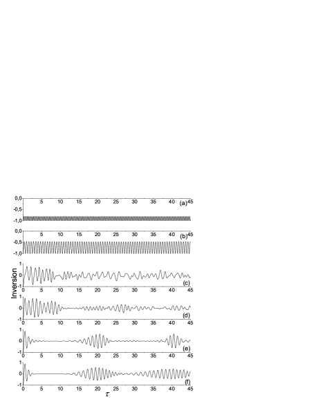
Figure 1: Rabi oscillations of the inversion for a QD exposed to the coherent state of light with $\langle{n(0)}{\rangle=9}$ and $\xi=0.2$ (a), $\xi=0.49$ (b), $\xi=0.53$ (c), $\xi=1.2$ (d), $\xi=3.5$ (e), $\xi=18.0$ (f).

V.1 Coherent states excitation

Figure 2: Rabi oscillations of the inversion for a QD exposed to the coherent state of light with $\langle{}n(0)\rangle=36$ and $\xi=0.53$ (a), $\xi=1.2$ (b), $\xi=18.0$ (c).

Let a ground–state QD be exposed to the elementary coherent state of light $\sum_{n=0}^{\infty}F(n)|n\rangle$, whereScully $F(n)=\exp{[-\langle{n(0)}\rangle/{2}]}\langle{n(0)}\rangle^{{n}/{2}}/{\sqrt{n!}}$. Then, initial conditions for Eqs. (32) are given by

$$B_{n}(0)=F(n)\,,\qquad A_{n}(0)=0\,.$$ (52)

Figures 1 and 2 show calculations of the inversion in a lossless QD as a function of the dimensionless time $\tau=|g|t$ at the exact synchronism ($\delta=0$) for two different initial photon mean numbers $\langle{n(0)}\rangle$ and for several values of parameter $\xi$. Our calculations demonstrate the appearance of two completely different oscillatory regimes in the Rabi oscillations. The first one manifests itself at $\xi<0.5$ and is characterized by periodic oscillations of the inversion within the range $-1\leq{w(t)}<{0}$ (see Figs. 1a, 1b). Thus, in this regime the inverted population is unreachable. On the contrary, in the second regime, at $\xi>0.5$, the inversion oscillates in the range $-1\leq{w(t)}\leq{1}$ (Figs. 1c–1f and Fig. 2). These two regimes of the Rabi effect are separated by the bifurcation which occurs at $\xi={0.5}$ for both types of incident coherent states (compare Figs. 1b and 1c).

In the limit $\xi\rightarrow{\infty}$ ($\Delta\omega\rightarrow 0$) the contribution of terms $O(\Delta\omega)$ in Eqs. (32) is small. The neglect these terms corresponds to the elimination of the local field effect. In this case the system (32) is reduced to that follows from the standard JC model Scully , allowing thus the analytical solution:

$$w(t)= - \sum\limits_{n=0}^{\infty}(B_{n+1}(0))^{2}\left[\frac{\delta^{2}}{\Omega_{n}^{2}}+\frac{4|g|^{2}(n+1)}{\Omega_{n}^{2}}\cos(\Omega_{n}t)\right]$$ (53)

$$- |B_{0}(0)|^{2}\,,$$ (54)

where $\Omega_{n}=\sqrt{\delta^{2}+4|g|^{2}(n+1)}$. The fundamental effect predicted by this solution is the collapse–revivals phenomenon in the time evolution of the inversion Scully . We have found that at $\xi\geq{18}$ the numerical simulation by Eqs. (32) leads to the same result as analytics (54), see Fig. 1f. In the case $\xi\rightarrow{0}$ the amplitude of Rabi oscillations tends to zero and $w(t)\approx-1$.

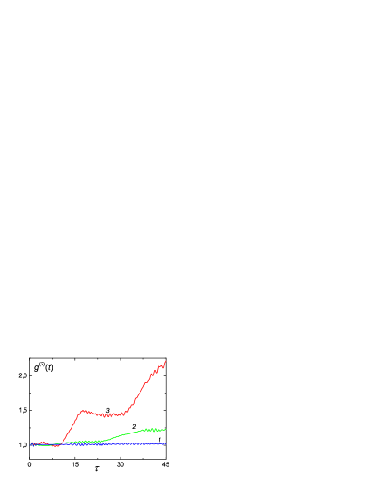
Figure 3: The second order time–zero correlation function $g^{(2)}(t)$ of QD exposed to the coherent state of light with $\langle{n(0)}{\rangle{=}9}$ and $\xi=18.0$ (1), $\xi=3.5$ (2), $\xi=1.2$ (3)

For a single QD imposed to classical light the appearance of two oscillatory regimes in Rabi oscillations separated by the bifurcation at $\xi=0.5$ has been predicted in Ref. magyar04, . Accordingly to [magyar04, ], the region $\xi>0.5$ corresponds to periodic anharmonic oscillations of the inversion. As different from that, in a QD exposed to quantum light the collapse–revivals phenomenon takes place in this region, see Figs. 1c–f and 2. As Figs. 1f and 2c demonstrate, the collapse and the revivals in the vicinity of the bifurcation are deformed and turn out to be drastically different from those predicted by the solution (54).

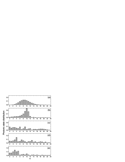
Figure 4: Photonic state distribution in a QD exposed to coherent light with $\langle n(0)\rangle=9$ for $\xi=1.2$ and $\tau=0$ (a), $\tau=8.5$ (b), $\tau=14.5$ (c), $\tau=31$ (d), $\tau=40$ (e).

The collapse–revivals effect in the time evolution of the inversion disappears completely in the range $\xi<0.5$ (see Figs. 1a–b), where the Rabi effect picture turns out to be identical to the case of QD excited by classical light magyar04 .

Let us estimate material parameters which provide observability of the effects predicted. For a spherical InGaAs QD with 6 nm radius the dipole moment can be estimatedref05 as $\mu\approx 12$ Debye. For this QD we obtain $\hbar\Delta\omega\approx 0.1$ meV. Then, for the range of $\xi$ presented in Fig. 1, from $\xi=0.2$ to $\xi=18$, we obtain $\hbar{\Omega_{\langle n\rangle}}\approx 0.02$ and $\hbar{\Omega_{\langle n\rangle}}\approx 2$ meV, respectively. These values are of the same order as the excitonic Rabi splitting measured in recent single QD spectroscopy experiments, see Refs. kamada, ; Yoshie_nature, . On the other hand, Refs. birkedal_SM02, ; bayer_prb02, ; borri_prb05, ; silverman_apl06, report the QD exciton linewidth $\Gamma_{{\rm hom}}$ of the order of 1 $\mu$eV below the temperature 10 K and laying in the range 4 to 10 $\mu$eV at $T=20$ K. Thus, the precondition to observe the strong coupling regime, $\hbar{\Omega_{\langle n\rangle}}\gg\Gamma_{{\rm hom}}$, is fulfilled for the given range of $\xi$.

An important feature of the Rabi effect in quantum light is the variation of the light statistics during the interaction with a quantum oscillator (QD). We shall characterize the variation by the second–order time–zero correlation function and the photonic state distribution defined by Eqs. (51) and (49), respectively. These characteristics at different $\xi$ are depicted in Figs. 3 and 4. One can see that at large $\xi\geq{}18$ the function $g^{(2)}(t)$ oscillates around unit in agreement with the standard JC modelScully , see curve 1 in Fig. 3. The situation is changed in the vicinity of the bifurcation as it is presented by curves 2 and 3 in that figure. As one can see, at $\xi=1.2$ the light statistics becomes super–Poisonnian. The correlation function $g^{(2)}(t)$ demonstrates the increase in time imposed to small-amplitude oscillations. These oscillations correspond to regions of revivals in the time evolution of the inversion (compare curve 3 in Fig. 3 and Fig. 1d). It should be noted that below the bifurcation threshold, at $\xi\leq{0.5}$, $g^{(2)}(t)$ oscillates in the vicinity of unity too.

Fig. 4 presents the photonic state distribution $p(n,t)$ for different time points at the given $\xi=1.2$. The figure illustrates consecutive transformation of the initially Poissonian distribution (Fig. 4a) into the super–Poisonnian one in the course of time, see Figs. 4c–d. The transformation corresponds to the increase in $g^{(2)}(t)$ illustrated by curve 3 in Fig. 3. Let us stress that the standard JC model predicts the photon statistics remaining Poisson as it takes place in our case only at large $\xi$ (curve 1 in Fig. 3). Our calculation also show that in the region $\xi<0.5$ the photon distribution $p(n,t)$ does not depend on time and remains Poissonian. The invariability of the coherent light statistics in the limit $\xi\rightarrow{0}$ corresponds to the absence of the component $\nu=1$ in Eq. (46).

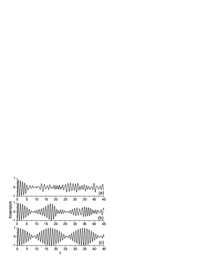
Figure 5: Rabi oscillations of the inversion for the QD exposed to the Fock qubit for $\xi=1.2$ (a), $\xi=8.0$ (b), $\xi=55.0$ (c).

V.2 QD interaction with Fock qubits

Let a ground-state QD interacts with electromagnetic field given by the Fock qubit (47). Then the initial conditions for Eqs. (32) are given by

$${A}_{n}(0)=0\,,\quad{B}_{n}(0)=\delta_{n,N}\beta_{N}+\delta_{n,N+1}\beta_{N+1}\,,$$ (55)

Further we restrict ourselves to the Fock qubit with $N=6$ assuming $\beta_{N}=\beta_{N+1}=\sqrt{1/2}$.

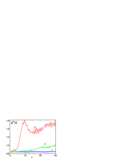
Figure 6: Second order time-zero correlation function $g^{(2)}(t)$ of the QD exposed to the Fock qubit with $N=6$ and $\xi=55.0$ $(\textsl{1})$, $\xi=8.0$ $(\textsl{2})$, $\xi=1.2$ $(\textsl{3})$.

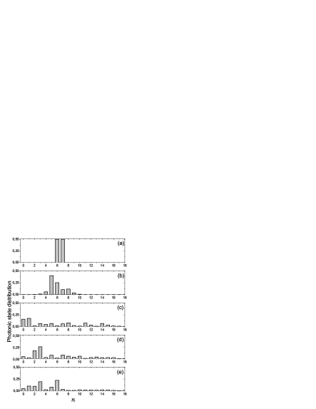
Figure 7: Photonic state distribution of the QD exposed to the Fock qubit for $\xi=1.2$ and $\tau=0$ (a), $\tau=5.19$ (b), $\tau=14.5$ (c), $\tau=29.6$ (d), $\tau=40.1$ (e).

Calculations of time evolution of the inversion for different values of $\xi$ are shown in Fig. 5. At large $\xi$ (Fig. 5c) the local field effect is eliminated: In agreement with the solution (54) the inversion exhibits harmonic modulation of the oscillation amplitude within the range $w\in[-1,1]$. The oscillation frequency is equal to $(\Omega_{N}+\Omega_{N+1})/2$ while the frequency of the modulation is given by $(\Omega_{N}-\Omega_{N+1})/2$. With the parameter $\xi$ decrease the modulation becomes non–harmonic.

The next two figures, 6 and 7, illustrate the change of the light statistics due to interaction with QDs. The time evolution of the correlation function $g^{(2)}(t)$ is depicted in Fiq. 6 for different values of $\xi$. Curve 1 demonstrates that, same as in Fig. 3 and in agreement with the standard JC model, at large $\xi$ ($\xi>55$) the correlation function oscillates in the vicinity of its initial value. Curve 3 shows transformation of the sub-Poissonian statistics ($g^{(2)}(t)<1$) into the super-Poissonian one ($g^{(2)}(t)>1$) with a pronounced maximum followed by irregular oscillations. Analogous but essentially smoothed behavior is observed at larger $\xi$ (curve 2).

Figure 7 presents calculations of the photonic state distribution $p(n,t)$ for $\xi=1.2$ (curve 3 in Fig. 6) in different points of time. The standard JC model when describes the interaction of Fock qubit with two–level system, predicts variation of those probabilities $p(n,t)$ (49) that correspond to Fock states with $n=N,N\pm 1$ numbers of photons. As different from that, the incorporation of the local–field effect leads to the appearance in the distribution of states $|n\rangle$ with photon numbers both smaller and larger than present in the initial Fock qubit (Fig.7a). Probabilities of these states are redistributed (Figs. 7b,c) with time, and light statistics became irregular which signifies the transformation of the photonic state distribution (Figs. 7d,e). In turn this affects the Rabi oscillations picture and the second order correlation function $g^{(2)}(t)$ (compare Figs. 5a and 6, curve 3).

V.3 Vacuum Rabi oscillations

The vacuum Rabi oscillations characterize interaction of an excited–state QD with electromagnetic vacuum. The initial conditions for Eqs. (32) in that case are given by $B_{n}(0)=0,A_{n}(0)=\delta_{n,0}$. Numerical solution of this system leads to the time–harmonic oscillations of the inversion. This agrees with the analytical solution of the system at $\Delta\omega=0$ given by the standard sinusoidal lawScully :

$$w(t)=\frac{\delta^{2}}{\Omega_{0}^{2}}+\frac{4|g|^{2}}{\Omega_{0}^{2}}\cos(\Omega_{0}t)\,.$$ (56)

The result can easily be understood from that the vacuum states, like a single Fock state, have zero observable electric field. Therefore, such states do not induce in QDs observable polarization and, consequently, frequency shift. For the same reason, zero frequency shift is inherent to single–photon states, as it has been revealed under some simplifying assumptions in Ref. maxim_pra_02, .

VI Discussion

The standard JC model describing the interaction between single–mode quantum electromagnetic field and two–level system predicts the collapse–revivals picture of the time evolution of the level population. The basic physical result of the analysis presented in our paper is a significant modification of the Rabi effect due to the local–field induced depolarization of a QD imposed to quantum light. Two oscillatory regimes with drastically different characteristics arise. In the first regime the time modulation of the population (the collapse and revivals) is suppressed and the QD population inversion is found negative. This indicates that trajectories of charge carriers confined by the QD occupy a finite volume in the phase space. In the second oscillatory regime the revivals appear, however they are found deformed and significantly different from that predicted by the standard JC model. The trajectories of charge carriers occupy the entire phase space. Both regimes of oscillations demonstrate the non–isochronous dependence on the coherent field strength.

Two regimes of the Rabi oscillations indicate the appearance of two types of motion of the QD exciton. The first one is a superposition of time-harmonic oscillations with the Rabi frequencies $\Omega_{n}=g\sqrt{N+1}$, while the second type is presented by the frequency band $|\omega_{p}-\omega_{0}|<2\Delta\omega$ . The resulting exciton motion is thus determined by a nonlinear superposition of these two types of motion.

The first mechanism of the motion is conventional for the Rabi effect; physically it originates from dressing of the QD exciton by the incident field photons. This type of motion dominates at large strengths of the incident field, when $\Omega_{\langle{n}\rangle}\gg\Delta\omega$. With the light–QD coupling constant (and correspondingly $\Omega_{\langle{n}\rangle}$) decrease, the role of the second type of motion grows in importance. The reason for this is the electron–hole correlations resulting from the exchange interaction. It can be interpreted as the QD exciton dressing by virtual photons. This regime becomes dominating in the comparatively weak fields, when $\Omega_{\langle{n}\rangle}\leq\Delta\omega$. Thus, the reduction of the threshold of the acting field strength needed for the Rabi oscillations appearance, recently observed experimentallymitsumori_05 , can be attributed as a local–field effect. The experimentmitsumori_05 has also elucidated the non-isochronism of excitonic Rabi oscillations that can be treated as the local–field effect as well; see the relation (37) and numerical calculations reported in Ref. [magyar04, ].

It should be noted that two oscillatory regimes in the Rabi effect may appear in other quantum systems where additional interaction mechanisms exist. As an example, consider a two–component Bose–Einstein condensate with radio-frequency coupling of two separate hyperfine statesdeconink_04 . Temporal evolution of this system is governed by the coupled Gross–Pitaevskii equations, which are similar to those derived in Sec. II.2. The equations combine both linear and nonlinear couplings. The linear coupling constant characterizes the interaction between the system and the electric field, while the nonlinear one accounts for the interaction between intra- and inter- species of the condensatedeconink_04 . Dependently on ratio of the coupling parameters, the Rabi oscillations between the condensate components may exhibit both well–ordered and chaotic behavior deconink_04 , similar to that depicted in Fig. 1a,b. The formation of the Bardeen–Cooper–Schrieffer state in the fermionic alkali gases cooled bellow degeneracy [barankov_04, ] can serve as another example. In that system, the time modulation of coupling constant leads to the Rabi oscillations of the energy gapbarankov_ref with two oscillatory regimes. The trajectories of individual Cooper pairs occupy a finite volume in the phase space in the first regime and the entire phase space in the second one.

Now, let us turn to the weak–field case. The the depolarization induced local field is predicted to entail in a QD exposed to an arbitrary photonic state a fine structure of the effective scattering cross–section. Instead of a single line of the frequency $\omega_{0}$, a duplet is appeared with one component shifted by a value $\Delta\omega$. The shifted component is due to electron–hole correlations, see Eq. (35). The correlations change the QD state and, consequently, provide the inelastic channel of the light scattering. The elastic scattering channel is formed by light states inducing zero observable polarization and, consequently, zero frequency shift, such as Fock states, vacuum states, etc. Now we take into account the relation $\langle{\bf\hat{P}}\rangle=4\pi{\alpha}\langle{\bf\hat{E}}_{0}\rangle$, which couples observable polarization and mean value of the incident field; the quantity $\bf{\hat{E}}_{0}$ is defined through the relation $\widehat{\bm{\mathcal{E}}}{}_{0}(\mathbf{t})=\int_{o}^{\infty}\widehat{\mathbf{E}}_{0}(\mathbf{r},\omega)d\omega+\rm{H.c}$. The scalar coefficient $\alpha$ is the QD polarizability of a spherical QD. Therefore, we conclude that the elastic scattering channel is formed by incident field with zero mean value (incoherent component of the electromagnetic field). Correspondingly, the coherent field component is scattered through inelastic channel. As follows from the solution (46), the elastic channel is not manifested for pure coherent light (the Glauber state).

Let us discuss now the local–field induced alteration of the quantum light statistics. As an example we consider the Fock qubit (47) as the incident field state. For the case $\Delta\omega=0$ the photonic state distribution is given by

$$p(n,t) = \delta_{n,N-1}|A_{N-1}(t)|^{2}+\delta_{n,N}(|A_{N}(t)|^{2}$$

$$+|B_{N}(t)|^{2})+\delta_{n,N+1}|B_{N+1}(t)|^{2}\,,$$ (57)

where $A_{n}(t)$ and $B_{n}(t)$ are the exact solutions of Eqs. (32) at $\Delta\omega=0$, see, e.g. Ref. Scully, . It is seen that the Fock states with photon numbers $n=N,N\pm 1$ are only presented in the distribution. The probability amplitudes of these states oscillate with the corresponding Rabi frequencies, $\Omega_{n=N,N\pm 1}$. In addition to this set, extra Fock states with both smaller and larger photon numbers are appeared in the photonic state distribution $p(n,t)$ as the local–field effect, See Fig. 7. Therefore, a bigger number of Fock states than presented in the initial Fock qubit, broaden the frequency spectrum of Rabi oscillations, providing thus the chaotic time evolution of the inversion.

It should be noted that the variation in the quantum light statistics occurs even in the weak–field limit $g\rightarrow{0}$. To illustrate that, consider the observable polarization of the QD exciton defined in the time domain as

$$\langle{\widehat{\bm{\mathcal{P}}}}\rangle = \frac{1}{V}{\bm{\mu}^{*}}\sum\limits_{\{n_{q}\}}A_{\{n_{q}\}}B_{\{n_{q}\}}^{*}{\rm e}^{-i\omega_{0}t}+\rm{c.c}\,.$$ (58)

Using Eq. (44) we couple the polarization in the frequency domain with the complex–valued amplitude of the mean incident field:

$$\langle{\bf\hat{P}}\rangle = \frac{|{\bm{\mu}}|^{2}/\hbar{V}}{\omega_{0}-\omega+\Delta\omega-i0}\langle{\bf\hat{E}}_{0}\rangle\,.$$ (59)

Then, after some simple manipulations we express the quantum fluctuations of the QD polarization by

$${\bf\hat{P}}-\langle{\bf\hat{P}}\rangle = \frac{|{\bm{\mu}}|^{2}/\hbar{V}}{\omega_{0}-\omega-i0}\left({\bf\hat{E}}_{0}-\langle{\bf\hat{E}}_{0}\rangle\right)\,.$$ (60)

From Eqs. (59) and (60) follows that the QD electromagnetic responses to the mean electric field and to its quantum fluctuation are different: the response resonant frequency is shifted by the value $\Delta\omega$ in the former case [relation (59) ] and remains unshifted in the later one, as given by relation (60). This indicates that the effective polarizability of a QD is an operator in the space of quantum states of light. It should be pointed out that this property is responsible for the alteration of the photonic state distribution in the weak–field regime and is entirely a local–field effect. Note that the notions ”strong (weak) coupling regime” and ”strong (weak) field regime” are not identical as applied to QDs. To illustrate this statement, we express from Eqs. (59) and (60) the polarization operator in the weak–field limit:

$${\bf\hat{P}} = \frac{|{\bm{\mu}}|^{2}/\hbar{V}}{\omega_{0}-\omega-i0}\left({\bf\hat{E}}_{0}-\frac{\Delta\omega{\langle{\bf\hat{E}}_{0}\rangle}}{\omega_{0}-\omega+\Delta\omega-i0}\right)\,.\,\,$$ (61)

This equation is linear in the incident field but includes a term quadratic in the oscillator strength, $O(|\bm{\mu}|^{4})$. Nonlinearity of that type violates the weak coupling regime. The splitting of the QD-exciton spectral line dictated by Eq. (60) is a manifestation of the strong light-matter coupling in the weak incident–field regime. Thus, the light–QD interaction is characterized by two coupling parameters, the standard Rabi–frequency and a new one, the depolarization shift $\Delta\omega$.

VII Conclusions

In the paper we have developed a theory of the electromagnetic response of a single QD exposed to quantum light, corrected to the local–field effects. The theory exploits the two-level model of QD with both linear and nonlinear coupling of excited and ground states. The nonlinear coupling is provided by the local field influence. Based on the microscopic Hamiltonian accounting for the electron–hole exchange interaction, an effective two–body Hamiltonian has been derived and expressed in terms of the incident electric field, with a separate term responsible for the local–field impact. The quantum equations of motion have been formulated and solved with this Hamiltonian for different types of the QD excitation, such as Fock qubit, coherent state, vacuum state and arbitrary state of quantum light.

For a QD exposed to coherent light we predict two oscillatory regimes in the Rabi oscillations separated by the bifurcation. In the first regime, the standard collapse–revivals phenomenon do not reveal itself and the QD inversion is found negative. In the second regime, the collapse–revivals picture is found to be strongly distorted as compared with that predicted by the standard JC model. The model developed can easily be extended to systems of other physical nature exposed to a strong electromagnetic excitation. In particular, we expect manifestation of the local–field effects in Bose–Einstein condensates deconink_04 and fermionic alkai gases cooled below the degeneracy barankov_04 .

We have also demonstrated that the local–field correction alters the light statistics even in the weak–field limit. This is because the local fields give rise to the inelastic scattering channel for the coherent light component. As a result, coherent and incoherent light components interact with QD on different frequencies separated by the depolarization shift $\Delta\omega$. In other words, the local fields eliminate the frequency degeneracy between these components of the incident light.

Note that our model does not account for the dephasing. Accordingly to recent experimental measurements Borri_prb02 ; borri_prb05 and theoretical estimates forstner_03 ; dizhu_05 , the electron–phonon interaction is the dominant mechanism of the dephasing in QDs. Thus, the further development of the theory presented requires this dephasing mechanism incorporation. A next step is generalization of our model to multi–level systems. Among them, the systems with dark excitons interacting with weak probe pulse in the self–consistent transparency regime fleischhauer_05 are of special interest.

In the paper we have considered an isolated QD. The generalization of the theory developed to the case of QD ensembles (excitonic composites), such as self–organized lattices of ordered QD molecules mano_04 and 1D–ordered (In, Ga)As QD arrays lippen_04 , is of special interest. One can expect that dipole–dipole interactions between QDs will manifest itself in a periodic transfer of excited state between QDs resulting thus in the collective Rabi oscillations — Rabi waves.

Appendix A Depolarization shift for the spherical QD

For a spherical QD, the formulae (29) is reduced to

$$\Delta\omega=\frac{4\pi}{3\hbar V}|{\bm{\mu}}|^{2}{\rm Tr}(\widetilde{\underline{N}})\,.$$ (62)

Using the expression (22) we obtain

$${\rm Tr}(\widetilde{\underline{N}}) = \frac{V}{4\pi}\int\limits_{V}\!\!|\zeta(\textbf{r}^{\prime})|^{2}\int\limits_{V}\!\!|\zeta(\textbf{r})|^{2}\nabla^{2}\left(\frac{1}{|\textbf{r}-\textbf{r}^{\prime}|}\right)d^{3}\textbf{r}d^{3}\textbf{r}^{\prime}$$ (63)

$$= V\int\limits_{V}\!\!\int\limits_{V}\!\!|\zeta(\textbf{r}^{\prime})|^{2}\zeta(\textbf{r})|^{2}\delta(\textbf{r}-\textbf{r}^{\prime})d^{3}\textbf{r}d^{3}\textbf{r}^{\prime}$$ (64)

$$= V\int\limits_{V}|\zeta(\textbf{r})|^{4}d^{3}\textbf{r}\,.$$ (65)

Consider the 1s state. The normalized wavefunction in this case is given by haug_b94

$$\zeta(\textbf{r})=\frac{1}{R\sqrt{2\rho}}J_{1/2}\left(\pi\frac{\rho}{R}\right)\,,$$ (66)

where $J_{\nu}(\dots)$ is the Bessel function, $\rho$ is the spherical coordinate and $R$ is the QD radius. Inserting (66) into (63) and integrating the resulting expression, we derive the correction to the depolarization shift (62)

$${\rm Tr}(\widetilde{\underline{N}})=\frac{4\pi}{3}\int\limits_{0}^{\pi}\frac{\sin^{4}x}{x^{2}}dx\approx 2.81\,.$$ (67)

References

- (1) M. O. Scully and M. S. Zubairy, Quantum Optics (University Press, Cambridge, 2001).
- (2) D. Bimberg, M. Grundmann, and N. N. Ledentsov, Quantum dot heterostructures. (John Wiley & Sons, Chichester, 1999).
- (3) Single quantum dots, Topics of applied physics, edited by P. Michler (Springer-Verlag Berlin, Heidelberg, 2000)
- (4) M. Kasevish, Science 298, 1363 (2002).
- (5) B. Lounis and M. Orrit, Rep. Prog. Phys. 68, 1129 (2005).
- (6) S. Brattke, B. T. H. Varcoe, and H. Walther, Phys. Rev. Lett. 86, 3534 (2001)
- (7) C. K. Law and J. H. Eberly, Phys. Rev. Lett. 76, 1055 (1996).
- (8) S. Ya. Kilin, Usp. Fiz. Nauk 169, 507 (1999) [Phys. Usp. 42, 435 (1999)].
- (9) I. V. Bagratin, B. A. Grishanin, and V. N. Zadkov, Usp. Fiz. Nauk 171, 625 (2001) [Phys. Usp. 44, 597 (2001)].
- (10) Y. A. Wheeler and W. H. Zurek, Qunatum theory of measurment, (Princenton Univ. Press, 1983).
- (11) E. T. Jaynes and F. W. Cummings, Proc. IEEE 51, 89 (1963).
- (12) Y. Yang, J. Xu, G. Li and, H.Chen, Phys. Rev. A 69, 053406 (2004).
- (13) M. Lewenstein, L. You, J. Cooper and, K. Burnett, Phys. Rev. A 50, 2207 (1994).
- (14) Weiping Zhang and D. F. Walls, Phys. Rev. A49, 3799 (1994).
- (15) Ka-Di Zhu, Zhuo-Jie Wu, Xiao-Zhong Yuan, and Hang Zheng, Phys. Rev. B71, 235312 (2005).
- (16) J. Förstner, C. Weber, J. Danckwerts, and A. Knorr, Phys. Rev. Lett. 91, 127401 (2003); J. Förstner, C. Weber, J. Danckwerts, and A. Knorr, Phys. Status. Solidi B, 238, 419 (2003).
- (17) M. Fleischhauer, A. Immamoglu, and J. P. Marangos, Rev. Mod. Phys. 77, 633 (2005).
- (18) H. T. Dung, L. Knoll and D.-G. Welsch, Phys. Rev. A66, 063810 (2002).
- (19) Th. Unold, K. Mueller, C. Lienau, Th. Elsaesser, and A. D. Wieck, Phys. Rev. Lett. 94, 137404 (2005).
- (20) T. H. Stievater, Xiaoqin Li, D. G. Steel, D. Gammon, D. S. Katzer, D. Park, C. Piermarocchi, and L. J. Sham, Phys. Rev. Lett. 87, 133603 (2001).
- (21) H. Kamada, H. Gotoh, J. Temmyo, T. Takagahara, and H. Ando, Phys. Rev. Lett. 87, 246401 (2001).
- (22) H. Htoon, T. Takagahara, D. Kulik, O. Baklenov, A. L. Holmes, Jr., and C. K. Shih Phys. Rev. Lett. 88, 087401 (2002).
- (23) A. Zrenner, E. Beham, S. Stufler, F. Findels, M. Bichler, G. Abstreiter, Nature 418, 612 (2002).
- (24) X. Li, Y. Wu, D. Steel, D. Gammon, T. H. Stievater, D. S. Katzer, D. Park, C. Piermarocchi, and L. J. Sham, Science 301, 5634 (2003).
- (25) Y. Mitsumori, A. Hasegawa, M. Sasaki, H. Maruki, and F. Minami Phys. Rev. B 71, 233305 (2005).
- (26) S. Schmitt-Rink, D. A. B. Miller, and D. S. Chemla, Phys. Rev. B 35, 8113 (1987).
- (27) B. Hanewinkel, A. Knorr, P. Thomas, and S. W. Koch, Phys. Rev. B 55, 13715 (1997).
- (28) G. Ya. Slepyan, S. A. Maksimenko, V. P. Kalosha, J. Herrmann, N. N. Ledentsov, I. L. Krestnikov, Zh. I. Alferov, and D. Bimberg, Phys. Rev. B 59, 12275 (1999).
- (29) S. A. Maksimenko, G. Ya. Slepyan, V. P. Kalosha, S. V. Maly, N. N. Ledentsov, J. Herrmann, A. Hoffmann, D. Bimberg, and Zh. I. Alferov, J. Electron. Mater. 29, 494 (2000).
- (30) H. Ajiki, T. Tsuji, K. Kawano, and K. Cho, Phys. Rev. B 66, 245322 (2002).
- (31) S. V. Goupalov, Phys. Rev. B 68, 125311 (2003).
- (32) G. Ya. Slepyan et al., in Advances in Electromagnetics of Complex Media and Metamaterials, edited by S. Zouhdi et al. (Kluwer, Dordrecht, 2003), p. 385.
- (33) S. A. Maksimenko and G. Ya. Slepyan, in Encyclopedia of Nanoscience and Nanotechnology, edited by J. A. Schwarz et al. (Marcel Dekker, New York, 2004), p. 3097.
- (34) S.A. Maksimenko and G.Ya. Slepyan, in The Handbook of Nanotechnology: Nanometer Structure Theory, Modeling, and Simulation, edited by A. Lakhtakia (SPIE Press, Belingham, 2004), p. 145.
- (35) G. Ya. Slepyan, S. A. Maksimenko, A. Hoffmann and D. Bimberg, Phys. Rev. A 66, 063804 (2002).
- (36) G. Ya. Slepyan, A. Magyarov, S. A. Maksimenko, A. Hoffmann, and D. Bimberg, Phys. Rev. B70, 045320 (2004).
- (37) This approach is often utilized for the description of d-d interactions in atomic optics, see e.g. Ref. Zhang_94, .
- (38) V. B. Berestetskii, E. M. Lifshitz, and L. P. Pitaevskii, Quantum Electrodynamics, (Pergamon, Oxford, 1982).
- (39) Applicability of the Hartree–Fock–Bogoliubov approximation to our problem was discussed in previous publications under the phenomenological derivation of Hamiltonian (20), see Refs. maxim_pra_02, ; Maksimenko_ENN, .
- (40) K. Cho, Optical Response of Nanostructures: Microscopic Nonlocal Theory (Springer-Verlag, Berlin, 2003).
- (41) W. W. Chow and S. W. Koch, Semiconductor-Laser Fundamentals: Physics of the Gain Materials, (Springer-Verlag, Berlin, 1999).
- (42) H. Haug and S. W. Koch, Quantum theory of the optical and electronic properties of semiconductors, (World Scientific, Singapure 1994).
- (43) This expression is obtained by i) the exponent expansion into Taylor series, ii) utilizing the relations () and and iii) subsequent summations of the Taylor series.
- (44) M. Brune, S. Haroche, J. M. Raimond, L. Davidovich, and N. Zagury, Phys. Rev. A45, 5193 (1992).
- (45) The dipole moment in the expression for the depolarization shift (62) for InGaAs spherical QD can be estimated using the experimental data of Ref. [K.L. Silverman, R.P. Mirin, S.T. Cundiff, A.G. Normann, Appl. Phys. Lett. 82, 25, (2003)] where the value from 25 to 33 Debye were measured for the QDs with average lateral dimensions from 30 to 40 nm. Taking into account the theretical results concerning the dependence of the transition dipole moment on the QD surface area and shape [ A. Thänharrdt, C. Ell, G. Khitrova, H.M. Gibbs Phys. Rev. B65, 035327, (2002)], we can roughly estimate the dipole moment Debye for spherical QD with radius 6 nm.
- (46) T. Yoshie, A. Scherer, J. Hendrickson, G. Khitrova, H. M. Gibbs, G. Rupper, C. Ell, O. B. Shchekin, and D. G. Deppe, Nature 432, 11 (2004).
- (47) D. Birkedal, K. Leosson, and J. M. Hvam, Superlattices and Microstructures 31, 97 (2002).
- (48) P. Borri, W. Langbein, S. Schneider, U. Woggon, R. L. Sellin, D. Ouyang, and D. Bimberg, Phys. Rev. B 66, 081306(R) (2002).
- (49) P. Borri, W. Langbein, U. Woggon, V. Stavarache, D. Reuter, A.D. Wieck Phys. Rev. B, 71, 115328 (2005).
- (50) J. J. Berry, M. J. Stevens, R. P. Mirin, and K. L. Silverman, Appl. Phys. Lett. 88, 061114 (2006).
- (51) M. Bayer and A. Forchel, Phys. Rev. B65, 041308(R) (2002).
- (52) B. Deconinck, P. G. Kevrekidis, H. E. Nistazakis, and D. J. Frantzeskakis, Phys. Rev. A 70, 063605 (2004).
- (53) R. A. Barankov, L. S. Levitov, and B. Z. Spivak, Phys. Rev. Lett. 93, 160401 (2004).
- (54) Rabi oscillations of the energy gap correspond to the periodic creation and annihilation of the Cooper pairs.
- (55) T. Mano, R. Notzel, G. J. Hamhius, T. H. Eijkemans, and J. H. Wolter, J. Appl. Phys. 95, 109 (2004).
- (56) T. V. Lippen, R. Notzel, G. J. Hamhius, and J. H. Wolter, Appl. Phys. Lett. 85, 118 (2004).