Spatial and kinematic alignments between central and satellite halos

Abstract

Based on a cosmological N-body simulation we analyze spatial and kinematic alignments of satellite halos within six times the virial radius of group size host halos (${\,r_{\rm vir}}$). We measure three different types of spatial alignment: halo alignment between the orientation of the group central substructure (GCS) and the distribution of its satellites, radial alignment between the orientation of a satellite and the direction towards its GCS, and direct alignment between the orientation of the GCS and that of its satellites. In analogy we use the directions of satellite velocities and probe three further types of alignment: the radial velocity alignment between the satellite velocity and connecting line between satellite and GCS, the halo velocity alignment between the orientation of the GCS and satellite velocities and the auto velocity alignment between the satellites orientations and their velocities. We find that satellites are preferentially located along the major axis of the GCS within at least $6{\,r_{\rm vir}}$ (the range probed here). Furthermore, satellites preferentially point towards the GCS. The most pronounced signal is detected on small scales but a detectable signal extends out to $\sim 6{\,r_{\rm vir}}$. The direct alignment signal is weaker, however a systematic trend is visible at distances $\lesssim 2{\,r_{\rm vir}}$. All velocity alignments are highly significant on small scales. The halo velocity alignment is constant within $2{\,r_{\rm vir}}$ and declines rapidly beyond. The halo and the auto velocity alignments are maximal at small scales and disappear beyond 1 and $1.5{\,r_{\rm vir}}$ respectively. Our results suggest that the halo alignment reflects the filamentary large scale structure which extends far beyond the virial radii of the groups. In contrast, the main contribution to the radial alignment arises from the adjustment of the satellite orientations in the group tidal field. The projected data reveal good agreement with recent results derived from large galaxy surveys.

1. Introduction

Over the last decades observational and numerical evidence has substantiated the picture of a filamentary large-scale structure in the universe. In principle the large-scale tidal field is expected to induce large-scale correlations between the orientations of halos and galaxies that are embedded within these filaments (e.g., Pen et al., 2000; Croft & Metzler, 2000; Heavens et al., 2000; Catelan et al., 2001; Crittenden et al., 2001; Porciani et al., 2002; Jing, 2002). On the other hand, the subsequent accretion onto larger systems, such as groups and clusters of galaxies, may alter the orientations of these (sub-)structures in response to the local tidal field (Ciotti & Dutta, 1994; Lee et al., 2005). Cosmological N-body simulations provide a valuable tool to differentiate the various contributions to the halo/galaxy alignments within overdense regions.

Observationally, various types of alignment between galaxies and their environment have been detected on a wide range in scales, from super-cluster systems down to the distribution of the satellite galaxies in our Milky Way (MW). On cluster scales various different types of alignment are discussed in the literature : alignment between neighboring clusters (Binggeli, 1982; Ulmer et al., 1989; West, 1989; Plionis, 1994; Chambers et al., 2002), between brightest cluster galaxies (BCGs) and their parent clusters (Carter & Metcalfe, 1980; Binggeli, 1982; Struble, 1990; Rhee & Latour, 1991; Plionis & Basilakos, 2002), between the orientation of satellite galaxies and the orientation of the cluster (Dekel, 1985; Plionis et al., 2003), and between the orientation of satellite galaxies and the orientation of the BCG (Struble, 1990). According to these studies the typical scales over which clusters reveal signs for alignment range up to $10-50{\,h^{-1}\rm Mpc}$, which can be most naturally explained by the presence of filaments.

With large galaxy redshift surveys, such as the two-degree Field Galaxy Redshift Survey (2dFGRS, Colless et al., 2001) and the Sloan Digital Sky Survey (SDSS, York et al., 2000), it has recently also become possible to investigate alignments on group scales using large and homogeneous samples. This has resulted in robust detections of various alignments: Brainerd (2005), Yang et al. (2006) and Azzaro et al. (2007) all found that satellite galaxies are preferentially distributed along the major axes of their host galaxies, while Pereira & Kuhn (2005) and Agustsson & Brainerd (2006a) noticed that satellite galaxies tend to be oriented towards the galaxy at the center of the halo.

In contradiction to the studies above, Holmberg (1969) found that satellites around isolated late type galaxies preferentially lie along the minor axis of the disc. Subsequent studies, however, were unable to confirm this so-called ‘Holmberg effect’(Hawley & Peebles, 1975; Sharp et al., 1979; MacGillivray et al., 1982; Zaritsky et al., 1997). Recently Agustsson & Brainerd (2007) reported a Holmberg effect at large projected distances around blue host galaxies, while on smaller scales the satellites were found to be aligned with the major axis of their host galaxy and Bailin & Steinmetz (2005) claim that a careful selection of isolated late-type galaxies reveals the the tendency for the satellites to align with the minor axis of the galactic disc. Investigating the companions of M31 Koch & Grebel (2006) find little evidence for a Holmberg effect. Yet, the Milky Way (MW) seems to exhibit a Holmberg effect even on small scales, in that the 11 innermost MW satellites show a pronounced planar distribution oriented close to perpendicular to the MW disc (Lynden-Bell, 1982; Majewski, 1994; Kroupa et al., 2005; Kang et al., 2005; Libeskind et al., 2005).

Numerical simulations have been employed to test alignment on a similar range in scales, from super-clusters down to galaxy-satellite systems. All studies focusing on cluster size halos report a correlation in the orientations for distances of at least $10{\,h^{-1}\rm Mpc}$; some studies observe a positive alignment signal up to $100{\,h^{-1}\rm Mpc}$ (e.g., Onuora & Thomas, 2000; Faltenbacher et al., 2002, 2005; Hopkins et al., 2005; Kasun & Evrard, 2005; Basilakos et al., 2006). These findings are interpreted as the signature of the filamentary network which interconnects the clusters. The preferential accretion along these filaments causes the clusters to point towards each other. Also, for galaxy and group-sized halos a tendency to point toward neighboring halos is detected. According to Altay et al. (2006) the alignments for such intermediate mass objects are caused by tidal fields rather than accretion along the filaments. Consequently, the mechanisms responsible for the alignment of the orientations depend on halo mass. Further evidence for a mass dependence of alignment effects comes from the examination of the halos’ angular momenta. Bailin & Steinmetz (2005) and Aragón-Calvo et al. (2007) find that the spins of galaxy size halos tend to be parallel to the filaments whereas the spins of group-sized halos tend to be perpendicular. This behavior may originate in the relative sizes of halos with respect to the surrounding filaments.

On subhalo scales basically three different types of alignments have been discussed: the alignment of the overall subhalo distribution with the orientation of the host halo (e.g., Knebe et al., 2004; Zentner et al., 2005; Agustsson & Brainerd, 2006b; Kang et al., 2007; Libeskind et al., 2007), the alignment of the orientations of subhalos among each other (e.g., Lee et al., 2005) and, very recently, the orientation of the satellites with respect to the center of the host (Kuhlen et al., 2007; Pereira et al., 2007). Again, accretion along the filaments and the impact of tidal fields have been invoked as explanations for the former and the latter, respectively. Thus, on all scales tidal fields and accretion along filaments are considered to be the main contributers to the observed alignment signals. Here we attempt to isolate the different contributions. In particular we focus on the continuous transition from subhalo to halo scales meaning we examine the alignment of (sub)structure on distance scales between 0.3 and 6 times the virial of groups sized halos.

Faltenbacher et al. (2007, hereafter Paper I) applied the halo-based group finder of Yang et al. (2005) to the SDSS Data Release Four (DR4; Adelman-McCarthy et al., 2006) and carried out a study of the mutual alignments between central galaxies (BCG) and their satellites in group-sized halos. Using the same data set consisting of over $60000$ galaxies three different types of alignment have been investigated : (1) the ‘halo’ alignment between the orientations of the BCG and associated satellite distribution; (2) the ‘radial’ alignment between the direction given by the BCG-satellite connection line and the satellite orientation; (3) the ‘direct’ alignment between the orientations of the BCG and the satellites. The study presented in this paper focuses on the same types of alignment and is aimed to compare the observational results with theoretical expectations derived from N-body simulations.

There are a variety of dynamical processes which can contribute to the alignments of satellites associated with groups, the most important are: (1) a possible pre-adjustment of satellites in the filaments, which for distances of a few times the virial radius commonly point radially towards the group; (2) the preferential accretion along those filaments; (3) the change of the satellite orbits in the triaxial group potential well; (4) the continuous re-adjustment of satellite orientations as they orbit within the group. Basically, the first two points can be attributed to the large scale environment of the groups whereas the latter two are more closely associated with the impact of the group potential on small scales. The purpose of the present analysis is to separate the different contributions to the observed alignment signals, therefore we analyse the mutual orientations of satellites within 6 times the virial radius of the groups. Since the tidal forces are closely related to the dynamics of the satellites additional insight into the generation of alignment can be gained by considering the satellite velocities. Therefore, we also investigate the direction of the satellite velocities with respect to their orientations, which constitutes an indirect way to infer the impact of the dynamics onto the orientation of the satellites. A more direct way to work out the interplay between the dynamics and the orientations would be to trace the orbits of individual satellites, however such an approach goes beyond the scope of the present study.

The paper is organized as follows. In § 2 we introduce the simulation and describe the halo finding procedure. § 3 deals with some technical aspects, namely the determination of the size and orientation of the substructures. In § 4 we present the signals of the three dimensional spatial and velocity alignments and in § 5 we repeat the analysis based on projected data. Finally, we conclude with a summary in § 6.

2. Simulation and halo identification

For the present analysis we employ an N-body simulation of structure formation in a flat $\Lambda$CDM universe with a matter density $\Omega_{m}=0.3$, a Hubble parameter $h=H_{0}/(100\>{\rm km}\,{\rm s}^{-1}\,{\rm Mpc}^{-1})=0.7$, and a Harrison-Zeldovich initial power spectrum with normalization $\sigma_{8}=0.9$. The density field is sampled by $512^{3}$ particles within a $100{\,h^{-1}\rm Mpc}$ cube resulting in a mass resolution of $6.2\times 10^{8}{\,h^{-1}\rm M}_{\odot}$. The softening length was set to $\epsilon=10{\,h^{-1}\rm kpc}$, beyond which the gravitational force between two particles is exactly Newtonian. The density filed is evolved with 5000 time steps from an initial redshift of $z_{i}=72$ using a PPPM method. An extensive description of the simulation can be found in Jing & Suto (2002) where it is quoted as LCDMa realization.

As detailed in the following two paragraphs the host halos and its satellites are found in two subsequent steps with two different techniques, first the main halos are located thereafter the associated satellite halos are detected. In order to identify the host halos we first run a FoF algorithm (Davis et al., 1985) on the simulation output at $z=0$. We set the FoF linking length to 0.1 times the mean particle separation, which selects regions with an average overdensity of $\sim 3000$. Note that, this linking length is a factor of two smaller than the commonly used value of 0.2, consequently only the central part of the host halo (and occasionally large substructures) are selected. Subsequently, the virial radius, ${\,r_{\rm vir}}$, is defined as the radius of the sphere centered on the most bound FoF particle which includes a mean density of 101 times the critical density, and we simply define the virial mass of each halo as the mass within ${\,r_{\rm vir}}$. If the virial regions of two halos overlap, the lower mass halo is discarded. In what follows we only focus on the 515 halos with a virial mass in the range from $10^{13}{\,h^{-1}\rm M}_{\odot}$ to $5\times 10^{14}{\,h^{-1}\rm M}_{\odot}$ (corresponding to halos with more than 16,000 particles). Since this is the typical mass scale of galaxy groups, we will refer to these halos as ‘groups’.

In a second step we search for self-bound (sub)structures using the SKID halo finder (Stadel, 2001) applied to the particle distribution within group centric distances of $6{\,r_{\rm vir}}$. As discussed in Macciò et al. (2006) SKID adequately identifies the smallest resolvable substructures when using a linking length $l$ equal to twice the softening length, i.e. four times the spline softening length. We therefore adopt $l=20{\,h^{-1}\rm kpc}$. Throughout we will distinguish between “group central substructures” (GCSs), which are located at the center of our groups, and satellites which are all the other (sub)structures, no matter whether they lie within or beyond ${\,r_{\rm vir}}$. According to this definition every group hosts one, and only one, GCS at its center while it may have numerous satellites outside the volume occupied by the GCS. Satellites are allocated to all groups from which they are separated less than $6{\,r_{\rm vir}}$. Hence, a satellite may be assigned to more than one GCS.

3. Size and orientation of substructures

Before describing the computation of the orientation we determine the typical sizes of the GCSs and the satellites. Knowledge about the physical sizes of the (sub)structures provides a crucial link for the comparison to observational data.

3.1. Sizes of group central substructures

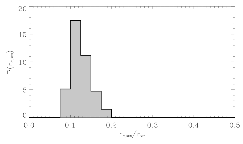
Figure 1.— Distribution of the spatial dispersion $r_{\sigma}$ of the group central substructure (GCS) in units of the virial radius. Satellites can only be resolved at radii larger than the size of the GCS.

The physical interpretation of the size of the GCS is not straightforward. For one thing, it depends on the SKID linking length used. However, for our purposes it is sufficient to notice that the GCS represents the dense inner region of the group which, largely due to numerical reasons, is free of substructure. Consequently, any radial dependence of satellite properties can only be probed down to the size of the GCS. In order to express the sizes of the GCS and the satellites we use the rms of the distances between the bound particles, $r_{\sigma}$. The advantage of this size measure is that it provides a direct estimate of the (momentary) size without having to make any assumption regarding the actual density distribution. In the case of an isolated NFW halo $r_{\sigma}\approx 0.5{\,r_{\rm vir}}$, with only a very weak dependence on the concentration parameter. Figure 1 displays the $r_{\sigma}$ distribution of the GCSs in units of the group’s virial radius, ${\,r_{\rm vir}}$. The distribution peaks at $0.11{\,r_{\rm vir}}$ and has a mean of $0.13{\,r_{\rm vir}}$.

3.2. Sizes of satellite halos

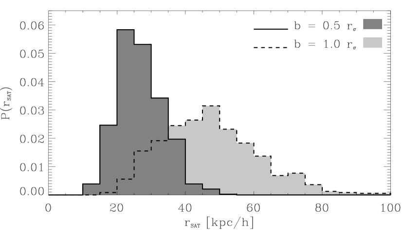
Figure 2.— Distribution of the radii of satellites found within the virial radius of the group. In this context radius refers to listed fraction (0.5, 1.0) of the satellites spatial dispersion $r_{\sigma}$. For example, the typical inner radii probed by the $b=0.5r_{\sigma}$ sample is $\sim 30{\,h^{-1}\rm kpc}$.

The aim of the present analysis is twofold: (1) to assess the impact of the group tidal field on the satellite orientations, and (2) to compare the alignment signals in our N-body simulation to observations of galaxy alignments. The impact of the group tidal field is stronger at larger satellite-centric radii. On the other hand, since galaxies reside at the centers of their dark matter halos, the central parts of the satellites are more of interest when comparing the alignment signals with those observed for galaxies. To meet both requirements we therefore measure the orientation of the satellite mass distribution within two radii. In analogy to the measurement of GCS sizes, we determine these radii with reference to the spatial dispersion $r_{\sigma}$. More precisely, we choose the particles within 1.0 and $0.5r_{\sigma}$ as the basic sets for the subsequent determination of the satellite orientation (see Section 3.3 below). Figure 2 displays the distributions of the corresponding physical sizes. The $0.5r_{\sigma}$ sample probes the matter distribution of the satellites within $\sim 25{\,h^{-1}\rm kpc}$, which is comparable to the sizes of elliptical galaxies. The mean, physical radii of the $1.0r_{\sigma}$ sample is $\sim 50{\,h^{-1}\rm kpc}$. If not quoted otherwise we will display the results for the $0.5r_{\sigma}$ sample, since this may most closely resemble the properties of observable galaxy distributions (outside of the very central part of the host halo).

3.3. Orientation

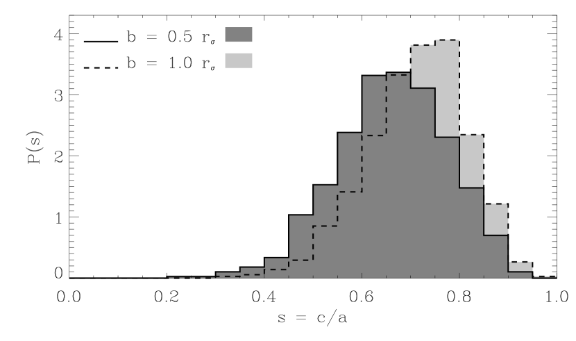
Figure 3.— Distribution of satellite shapes, represented by the ratio of shortest to the longest semi-major axis of the mass-ellipsoid ($s=c/a$). The colors correspond to the samples with different truncation radii as listed. With increasing size the halos become rounder. The distribution of the $b=0.5r_{\sigma}$ sample is rather symmetric, whereas for larger truncation radii there appears a slight asymmetry.

There are a few different ways found in the literature (e.g., Bullock, 2002; Jing & Suto, 2002; Bailin & Steinmetz, 2005; Kasun & Evrard, 2005; Allgood et al., 2006) to model halos as ellipsoids. They all differ in details, but most methods model halos using the eigenvectors from some form of the inertia tensor. The eigenvectors correspond to the direction of the major axes, and the eigenvalues to the lengths of the semi-major axes $a\geq b\geq c$. Following Allgood et al. (2006) we determine the main axes by iteratively computing the eigenvectors of the distance weighted inertia tensor.

$$I_{ij}=\sum_{k=1,N}{r_{ki}r_{kj}\over r^{2}_{k}}\ ,$$ (1)

where $r_{ki}$ denotes the $i$th component of the position vector of the $k$th particle with respect to the center of mass and

$$r_{k}=\sqrt{{x^{2}\over a^{2}}+{y^{2}\over b^{2}}+{z^{2}\over c^{2}}}$$ (2)

is the elliptical distance in the eigenvector coordinate system from the center to the $k$th particle. The square roots of the eigenvalues of the inertia tensor determine the axial ratios of the halo ($a:b:c=\sqrt{\lambda_{a}}:\sqrt{\lambda_{b}}:\sqrt{\lambda_{c}}$). The iteration is initialized by computing the eigenvalues of the inertia tensor for the spherically truncated halo. In the following iterations the length of the intermediate axis is kept unchanged and all bound particles within the ellipsoidal window determined by the eigenvalues of the foregoing iteration are used for the computation of the new inertia tensor. The iteration is completed when the eigenvectors have converged. The direction of the resulting major axis is identified as the orientation. The advantage of keeping the intermediate axis fixed is that the number of particles within the varying ellipsoidal windows remains almost constant. Instead, if the longest (shortest) axis is kept constant the number of particles within the ellipsoidal windows can decrease (increase) substantially during the iteration.

Note that we apply this truncation to all (sub)structures, both satellites and GCSs, and that the orientation of each sub(structure) is measured within this truncation radius. Throughout we only consider those sub(structures) that comprise at least 200 bound particles within the volume of the final ellipsoid (corresponding to a lower limit in mass of $\approx 10^{11}{\,h^{-1}\rm M}_{\odot}$). For the satellites this implies that a smaller truncation radius results in a smaller sample. For example, there are 772 $0.5r_{\sigma}$ satellites within the virial radii of our groups whereas the $1.0r_{\sigma}$ sample comprises 1431 satellites. Since all 515 GCSs contain more than 200 particles within $0.5r_{\sigma}$ their sample size is independent of the truncation radius used.

Figure 3 displays the distribution of the shape parameter $s=c/a$. The shading corresponds to different truncation radii as listed. There is a weak indication that satellites become more spherical with increasing truncation radii. A similar behavior was found for isolated halos (e.g., Jing & Suto, 2002; Allgood et al., 2006). As discussed by Allgood et al. (2006) the exact determination of individual shapes may need as many as 7000 particles, so that the resolution of the present simulation is not suited for the analysis of (sub)structure shapes. However, for the determination of the orientations, which is the focus of this paper, a particle limit of 200 can be considered conservative (cf., Jing, 2002; Pereira et al., 2007). A study examining the shapes of substructure in a single high-resolution Milky Way-sized halo can be found in Kuhlen et al. (2007).

4. Three dimensional Alignments

For both classes of objects, GCSs and satellites, the orientations are determined according to the approach described above. A third orientation-like quantity is given by the direction of the line connecting a GCS-satellite pair. Throughout we refer to the orientation of the GCS, the satellite and the connecting line as ${\mathbf{a}}_{\rm GCS}$, ${\mathbf{a}}_{\rm SAT}$ and ${\mathbf{r}}$, respectively. These quantities are unit vectors, such that the scalar product of two vectors yields the cosine of the angle between them. We will focus on three different types of alignment, (1) the halo alignment between the orientations of the GCSs and the connecting lines, (2) the radial alignment between the orientations of the satellites and the connecting lines and (3) the direct alignment between the orientation of the GCS and that of its satellites. In addition, we also consider various alignments based on the proper velocity, ${\mathbf{v}}$, of the satellite with respect to its GCS. In particular, we discuss (4) the radial velocity alignment between ${\mathbf{v}}$ and ${\mathbf{r}}$, (5) the halo velocity alignment between ${\mathbf{a}}_{\rm GCS}$ and ${\mathbf{v}}$, and finally (vi) the auto velocity alignment between the orientations, ${\mathbf{a}}_{\rm SAT}$, and velocities, ${\mathbf{v}}$, of the satellites. Here ${\mathbf{v}}$ is the unit vector indicating the direction of the proper velocity of the satellite (including the Hubble flow) relative to the host. Since all the other quantities also represent unit vectors the scalar products yield the cosines of the enclosed angles.

4.1. Halo alignment

Figure 4.— Mean values of the cosines of the angles between the orientations of the GCS and the connecting lines to the satellites, $\langle|{\mathbf{a}}_{\rm GCS}\!\cdot\!{\mathbf{r}}|\rangle\,$, as a function of $r/{\,r_{\rm vir}}$ for the $0.5r_{\sigma}$ sample. The dotted horizontal line indicates the mean values for an isotropic distribution. The error bars indicate the $95\%$ bootstrap confidence intervals within each distance bin.

In order to measure the alignment between the GCS and the satellite distribution we use ${\mathbf{a}}_{\rm GCS}$ and ${\mathbf{r}}$ (the orientation of the GCS and the position of the satellite with respect to its GCS). Figure 4 displays the radial dependence of $\langle|{\mathbf{a}}_{\rm GCS}\!\cdot\!{\mathbf{r}}|\rangle\,$ within $6{\,r_{\rm vir}}$, where $\langle\cdot\rangle$ denotes the mean value within a bin of $r/{\,r_{\rm vir}}$. The error bars indicate the $95\%$ bootstrap confidence intervals based on 1000 bootstrap samples for each distance bin. Over the entire range of distances probed, the mean values of the cosines deviate significantly from a isotropic distribution. The strength of the alignment, i.e. the deviation from $\langle|{\mathbf{a}}_{\rm GCS}\!\cdot\!{\mathbf{r}}|\rangle\,=0.5$, increases with group centric distance and reaches a maximum at $\sim 1.7{\,r_{\rm vir}}$. The subsequent decline, however, is very weak and even at $6{\,r_{\rm vir}}$ the alignment is still very pronounced ($\langle|{\mathbf{a}}_{\rm GCS}\!\cdot\!{\mathbf{r}}|\rangle\,\approx 0.55$), with no clear indication of a downward trend. The fact that there is strong alignment over such a long range suggests that the halo intrinsic alignment is closely connected to the filamentary structure in which the groups are embedded in. Since here we focus on the transition between group and environment dominated areas we do not aim to map out the entire range of the radial alignment.

The weakening of the signal at small scales may be attributed to the fact that the information about the filamentary origin is washed away once the satellites start to orbit within the groups (i.e., once non-linear effects kick in). Yet, the orientation of the group itself is closely correlated with the surrounding filamentary network, so that a residual alignment is maintained by the overall distribution of satellites orbiting in the potential well of the group (cf. Statler, 1987; Zentner et al., 2005; Kang et al., 2007). Additionally, if one assumes that filaments are approximately cylindrical in shape and the GCS is aligned with the orientation of the cylinder, then the mean angles between the orientation of the GCS and the satellites position become larger at smaller group-centric radii. In fact, at distances smaller than the radius of the cylinder the distribution will converge to isotropic. Finally, some contribution to the decrease of the alignment strength on small scales may come from the fact that satellites on nearly radial orbits are filtered out during their epicenter passage. They get severely stripped and consequently the number of particles that remains bound can easily fall below the detection criterion (minimum of 200 particles), thus weakening the alignment signal.

4.2. Radial alignment

Figure 5.— Same as Figure 4, but for the distributions of cosines between the satellite orientation and the connecting line to the GCS, $|{\mathbf{a}}_{\rm SAT}\!\cdot\!{\mathbf{r}}|$ for the $0.5$ and $1.0r_{\sigma}$ samples.

The radial alignment, $\langle|{\mathbf{a}}_{\rm SAT}\!\cdot\!{\mathbf{r}}|\rangle\,$, probes the orientations of individual satellites, ${\mathbf{a}}_{\rm SAT}$, relative to the direction pointing towards their GCS, ${\mathbf{r}}$. Figure 5 displays $\langle|{\mathbf{a}}_{\rm SAT}\!\cdot\!{\mathbf{r}}|\rangle\,$ for distances up to $6{\,r_{\rm vir}}$. The line styles represent different truncation radii of the satellites. Over the entire range of group-centric distances probed, the data reveal a significant anisotropic distribution. The signal is most pronounced on small scales, where it also shows a strong dependence on the truncation radii. The $1.0r_{\sigma}$ sample, which includes the behavior of the outer mass shells of the satellites, clearly exhibits a stronger deviation from isotropy. Within $\sim 1.5{\,r_{\rm vir}}$ there is a pronounced decline of the radial alignment signal, while it remains remarkably constant at larger radii. For distance in the range between $2-6{\,r_{\rm vir}}$ we detect a weak but significant signal, $\langle|{\mathbf{a}}_{\rm GCS}\!\cdot\!{\mathbf{a}}_{\rm SAT}|\rangle\,\approx 0.52$, inconsistent with isotropy at 95% confidence level in good agreement with Hahn et al. (2007). In a recent study, Kuhlen et al. (2007) detected no radial alignment for distances $\gtrsim 3{\,r_{\rm vir}}$. However, their analysis is based on a resimulation of a single galaxy-sized host halo. Since this halo is rather isolated, in that it has not experienced any major merger after redshift $z=1.7$, it is likely that its ambient filaments have already been drained.

At large distances satellites preferentially reside in filaments (as discussed in the context of Figure 4) which point radially towards the groups. Consequently, the signal on scales $\gtrsim 2{\,r_{\rm vir}}$ indicates an alignment between the satellite orientations and the filaments in which they are embedded. Such an alignment may be caused by accretion of matter along those filaments or by the local tidal fields generated by the mass distribution within the filaments. The group tidal field is not likely to be responsible for the observed large scale alignment signal due to its rapid decline with distance. On small scales, however, the tidal field can substantially alter the orientations of the satellites. As shown by Ciotti & Dutta (1994) the time scale on which a prolate satellite can adjust its orientation to the tidal field of a group is much shorter than the Hubble time, but longer than its intrinsic dynamical time. Therefore, the adjustment of the satellite orientations parallel to the gradients of the group potential offers a convincing explanation for a radial alignment signal on small scales. This perception is further supported by the dependence of the alignment strength on the truncation radii of the satellites. For the largest radii, which are strongest affected by tidal forces, the alignment signal is strongest.

4.3. Direct alignment

Figure 6.— Same as Figure 4, but for the distributions of cosines between the orientation of the satellites and the GCS, $|{\mathbf{a}}_{\rm GCS}\!\cdot\!{\mathbf{a}}_{\rm SAT}|$.

The strong signals for halo and radial alignment may lead to the expectation of a comparably pronounced signal for the direct alignment between the orientation of the GCS, ${\mathbf{a}}_{\rm GCS}$, and the orientations of its satellites, ${\mathbf{a}}_{\rm SAT}$. However, as can be seen in Figure 6, the signal is weak. There is only a weak trend for positive alignment up to $2{\,r_{\rm vir}}$. The significance found at distances between $1$ and $\sim 2{\,r_{\rm vir}}$ seems to be somewhat higher ($\sim 90\%$ confidence). Based on an analytical model Lee et al. (2005) predict a certain degree of parallel alignment between host and satellite orientations due to the evolution of the satellites within the tidal shear field of host. The signal for the direct alignment may be a relic of this effect.

To summarize, we find positive alignment signals for all three types of alignment tested here. However, they differ in strength and radial extent. The halo alignment is the strongest and reaches far beyond the virial radii of the groups ($\gtrsim 6{\,r_{\rm vir}}$). The radial alignment is most pronounced at small scales, where it reveals a strong dependence on the radial extent of the satellite over which its orientation has been measured. Although the radial alignment is weak beyond $\sim 1.5{\,r_{\rm vir}}$, the signal stays remarkably constant out to $\sim 6{\,r_{\rm vir}}$. Finally, the least prominent signal comes from the direct alignment. This ranking of the alignment strengths is in good agreement with the observational results reported in Paper I.

4.4. Alignments based on subhalo velocities

If tidal forces give rise to the radial alignment on small scales, as displayed in Fig. 5, the satellite orientations should be related to their actual velocities and the local gradients of the host potential. For instance a satellite moving radially towards the GCS will show an enhanced radial alignment since the gradient of the potential and the actual velocity are pointing in the same direction inducing an orientation in radial direction. On the other side the orientations of satellites moving perpendicular to the gravitational field (i.e. tangentially with respect to the GCS) will lie in between their velocities and the gradients of the potential well. To gain some more insight into the dynamical origin of the alignments, we include the directions of satellite velocities into the alignment study. We will consider three different kinds of alignments: the radial velocity alignment, $|{\mathbf{v}}\cdot{\mathbf{r}}|$, the halo velocity alignment $|{\mathbf{a}}_{\rm GCS}\cdot{\mathbf{v}}|$ and the auto velocity alignment $|{\mathbf{a}}_{\rm SAT}\cdot{\mathbf{v}}|$.

Figure 7.— Ratio of inward moving satellites, $f_{\rm in}=n_{\rm in}/(n_{\rm out}+n_{\rm in})$ for the $0.5r_{\sigma}$ sample. Error bars are Poisson.

To facilitate the interpretation of the velocity alignments, we split the satellites according to whether their net motion is inward (${\mathbf{v}}\!\cdot\!{\mathbf{r}}<0$) or outward (${\mathbf{v}}\!\cdot\!{\mathbf{r}}>0$) with respect to their group. Figure 7 shows the fraction of inward moving satellites, $f_{\rm in}$, as a function of their group centric distances. Note that $f_{\rm in}$ reaches a maximum around $\sim 2{\,r_{\rm vir}}$, beyond which the Hubble flow gradually starts to become more and more important. In fact, at sufficiently large radii, where the Hubble flow dominates, one expects that $f_{\rm in}=0$, and all satellites reveal an outward motion. For satellites that are in virial equilibrium within the group potential (i.e., at $r\lesssim{\,r_{\rm vir}}$), one expects roughly equal numbers of inward and outward moving systems (i.e., $f_{\rm in}=0.5$). However, on these small scales one has an additional contribution from the infall region around the group, causing $f_{\rm in}>0.5$. In addition, a substantial fraction of satellites get stripped below the detection limit (200 particles) at their peri-centric passage, so that they no longer contribute to the signal on their outward motion (cf., Faltenbacher & Mathews, 2007). At ${\,r_{\rm vir}}$, the outgoing satellite fraction is about 40%, which is (within the errors) consistent with the value $\sim 30\%$ determined by Wang et al. (2005). If one assumes an average ratio of 6:1 between apo- and peri-center distances for typical satellite orbits (Ghigna et al., 1998; van den Bosch et al., 1999) the majority of these satellites must have passed the central parts of the group before (cf., Diemand et al., 2007).

Figure 8.— Same as Figure 4, but for $\langle|{\mathbf{v}}\!\cdot\!{\mathbf{r}}|\rangle\,$. The upper, middle and lower panel displays the signal for all, the inward and the outward moving satellites, respectively.

The upper panel of Figure 8 displays the radial velocity alignment, $\langle|{\mathbf{v}}\!\cdot\!{\mathbf{r}}|\rangle\,$, as a function of $r/{\,r_{\rm vir}}$. $\langle|{\mathbf{v}}\!\cdot\!{\mathbf{r}}|\rangle\,>0.5$ indicates that the distribution of angles between ${\mathbf{r}}$ and ${\mathbf{v}}$ is not isotropic, instead, on average they preferentially point in radial directions. This behavior is in agreement with earlier studies of the velocity anisotropy of subhalos which is usually expressed by the anisotropy parameter $\beta=1-0.5(\sigma_{t}/\sigma_{r})^{2}$ (e.g., Binney & Tremaine, 1987), where $\sigma_{t}$ and $\sigma_{r}$ denote the velocity dispersions of the satellites in the tangential and radial direction, respectively. Note, $\langle|{\mathbf{v}}\!\cdot\!{\mathbf{r}}|\rangle\,$ is closely related to $\beta$. If one assumes a relaxed (steady-state) halo the above mentioned tendency towards radial motions translates into a higher radial velocity dispersion compared to the tangential one $\sigma_{r}>\sigma_{t1}=\sigma_{t}/\sqrt{2}$ (where $\sigma_{t1}$ and $\sigma_{t}$ are the one and two dimensional tangential velocity dispersions, respectively and tangential isotropy is assumed). Thus $\langle|{\mathbf{v}}\!\cdot\!{\mathbf{r}}|\rangle\,>0.5$ on small scales ($r\lesssim 2{\,r_{\rm vir}}$) suggest that $\sigma_{r}>\sigma_{t}/\sqrt{2}$, in good qualitative agreement with numerical simulations which have shown that $\beta>0$ for subhalos within the virial radius of their hosts. (Ghigna et al., 1998; Colín et al., 2000; Diemand et al., 2004).

In accordance with the spherical collapse model the signal extends out to $\sim 2{\,r_{\rm vir}}$, which roughly reflects the distance of turnaround. At $2.5{\,r_{\rm vir}}$ the distribution is close to isotropic suggesting that at these distances the impact of the group potential is negligible and the satellite motions are dominated by local potential variations arising from the filaments and dark matter halos within these filaments. Note that the presence of this filamentary structure in the vicinity of groups is clearly evident from Figure 4. Finally, the increase of the radial velocity alignment on large scales, $\gtrsim 4{\,r_{\rm vir}}$, is simply due to the Hubble flow (i.e., $\langle|{\mathbf{v}}\!\cdot\!{\mathbf{r}}|\rangle\,\rightarrow 1$ at $r\rightarrow\infty$). The middle panel of Figure 8 shows $\langle|{\mathbf{v}}\!\cdot\!{\mathbf{r}}|\rangle\,$ for the inward moving satellites only. The radial trend within $2{\,r_{\rm vir}}$ is somewhat enhanced compared to the upper panel. At larger radii, the inward moving satellites have a velocity structure that is consistent with isotropy. The lower panel of Figure 8 reveals a marked difference in the behavior of $\langle|{\mathbf{v}}\!\cdot\!{\mathbf{r}}|\rangle\,$ for the outward moving satellites. It indicates a slightly radial trend for satellites within $1{\,r_{\rm vir}}$ which is much lower than seen in the upper two panels. Within $1-2{\,r_{\rm vir}}$ it drops below 0.5, indicating a preference for tangential velocities. Together with the information derived from Figure 7 this suggests that a substantial fraction of outward moving satellites located at $1-2{\,r_{\rm vir}}$ currently are close to their apo-center passage after having crossed the more central regions of the group. Finally, on large scales the outward moving satellites clearly reveal the Hubble flow.

Figure 9.— Same as Figure 4, but for $\langle|{\mathbf{a}}_{\rm GCS}\!\cdot\!{\mathbf{v}}|\rangle\,$.

Figure 9 displays the radial dependence of $\langle|{\mathbf{a}}_{\rm GCS}\!\cdot\!{\mathbf{v}}|\rangle\,$ which measures the cosines of the angels between the satellite velocities and the orientation of the GCS. On large scales the radial outward motion caused by the Hubble flow exceeds the internal velocities of the satellites within the filaments. Since the GCS is strongly aligned with these filaments over the entire radial range shown (cf. Figure 4), one has that $\langle|{\mathbf{a}}_{\rm GCS}\!\cdot\!{\mathbf{v}}|\rangle\,>0.5$ on scales where the Hubble flow becomes important ($\gtrsim 4{\,r_{\rm vir}}$). The strong alignment signal on small scales indicates that the satellites tend to move parallel to the orientation of the GCS. According to Tormen (1997) and Allgood et al. (2006) the principal axes of the velocity anisotropy tensor are strongly correlated with the principal axes of the satellite distribution. Therefore, the alignment found for $\langle|{\mathbf{a}}_{\rm GCS}\!\cdot\!{\mathbf{r}}|\rangle\,$ (Figure 4) actually implies an analogous signal for $\langle|{\mathbf{a}}_{\rm GCS}\!\cdot\!{\mathbf{v}}|\rangle\,$. However, in contrast to the halo alignment, $\langle|{\mathbf{a}}_{\rm GCS}\!\cdot\!{\mathbf{r}}|\rangle\,$, the velocity halo alignment, $\langle|{\mathbf{a}}_{\rm GCS}\!\cdot\!{\mathbf{v}}|\rangle\,$, only extends out to $\sim 1{\,r_{\rm vir}}$. Beyond this radius a substantial fraction of the satellites shows relatively large angles between their velocities and the orientation of the GCS which is consistent with the picture of tangential motions associated with the apo-center passage of the satellites, as discussed in the context of Figure 8.

Figure 10.— Same as Figure 4, but for the distributions of cosines between the satellites velocities and positions, $|{\mathbf{v}}\!\cdot\!{\mathbf{r}}|$.

Finally we consider the auto velocity alignment, $\langle|{\mathbf{a}}_{\rm SAT}\!\cdot\!{\mathbf{v}}|\rangle\,$, which reflects the distribution of the cosines between the satellite velocities and their orientations, $|{\mathbf{v}}\cdot{\mathbf{a}}_{\rm SAT}|$. Fig 10 displays the variation of $\langle|{\mathbf{a}}_{\rm SAT}\!\cdot\!{\mathbf{v}}|\rangle\,$ with $r/{\,r_{\rm vir}}$.

The signal for $\langle|{\mathbf{a}}_{\rm SAT}\!\cdot\!{\mathbf{v}}|\rangle\,$ shows a maximum at $0.7{\,r_{\rm vir}}$. At larger distances it decreases quickly. Beyond $1.5{\,r_{\rm vir}}$ it is roughly in agreement with an isotropic distribution. A possible reason for the slight central dip is, that satellites on their peri-center passages move perpendicular to the gradients of the group potential. Figure 5, however, revealed a preferential radial orientation of these satellites. Thus, during the peri-center passages the angles between satellite orientations and velocities can become large. The degree of the radial alignment depends on the ratio between the internal dynamical time of the satellite, with which it can adjust its orientation, and the duration of the peri-center passage. If the peri-center passage occurs too quickly the time may be too short for a ‘perfect’ radial alignment (cf., Kuhlen et al., 2007). On large scales ($1-2{\,r_{\rm vir}}$) a similar mechanism may take place. Above we have argued that within this distance range a substantial fraction of satellites are close to their apo-center passage. During this phase the velocities are again perpendicular to the gradient of the potential but, as indicated by Figure 5, the satellites are oriented radially. The comparison between the signal for $\langle|{\mathbf{a}}_{\rm SAT}\!\cdot\!{\mathbf{r}}|\rangle\,$ and $\langle|{\mathbf{a}}_{\rm SAT}\!\cdot\!{\mathbf{v}}|\rangle\,$ suggests that, in a statistical sense, the (spatial) radial alignment is maintained during the entire orbit of the satellite within the potential well of the groups, which in turn causes a suppression of $\langle|{\mathbf{a}}_{\rm SAT}\!\cdot\!{\mathbf{v}}|\rangle\,$, at its apo- and peri-center.

5. Projected Alignments

To facilitate a comparison with observations, in particular with the results presented in Paper I, we repeat the foregoing analysis using projected data, i.e. we project the particle distribution along one of the coordinate axes and compute the second moment of mass for the projected particle distribution. Accordingly, for the distances between GCS and satellites we use the projected values (all satellites within a sphere of $6{\,r_{\rm vir}}$ about the GCS are projected), which we label as $R$ (the physical distances are labelled as $r$).

Since the projections along the three Cartesian coordinate axes are independent we include all three projections of each host-satellite in our 2D sample. To reduce the contamination by satellites associated with massive ambient groups we exclude those host-satellite systems where another SKID group more massive than the GCS (which is most likely the center of an ambient host-satellite system) is found within a sphere of $6{\,r_{\rm vir}}$. After rejection of ‘contaminated’ groups we obtain 1034 and 543 satellites for the $1.0r_{\sigma}$ and $0.5r_{\sigma}$ samples with 3D distances to the GCS $\leq{\,r_{\rm vir}}$ (for all groups irrespective of their environment we found 1431 and 772, see § 3.3.) Furthermore, since (due to technical reasons) we project satellites located within a sphere of $6{\,r_{\rm vir}}$ the projected volume at large projected distances shrinks substantially. Therefore, we analyze the 2D data only for projected distances $\lesssim 3{\,r_{\rm vir}}$ which roughly resembles the projection of all satellites within a cylinder with a radius $3{\,r_{\rm vir}}$ and length of $10{\,r_{\rm vir}}$ along the ‘line of sight’. Thus, in an approximate manner, uncertainties in the determination of group membership based on redshift measurements are accounted for.

The resolution of the simulation does not permit to probe alignment below $0.3{\,r_{\rm vir}}$. Other authors (using semi-analytical techniques, e.g., Kang et al., 2007) have bypassed this problem by introducing so-called orphan galaxies, i.e. galaxies which are associated with the once most bound particle of a satellite halo which subsequently has become undetectable due to the stripping by tidal forces. Here we do not adopt this technique since it does not provide us with information about the orientation of a satellite. Both approaches, considering only satellite halos with a minimum number of particles and the introduction of orphan galaxies, have certain disadvantages. The former does not account for galaxies which are hosted by strongly stripped subhalos whereas the latter ignores the dynamical differences of galaxies and (once most bound) particles.

The application of a fixed lower particle limit excludes satellites from the analysis which still constitute distinct objects. In particular satellites which are strongly tidally stripped may fall below the selection criterion even if the galaxy, which is assumed to sit at the center, may still be observable. Thus, we caution that our satellite sample may be somewhat biased toward more recently accreted satellites compared to a hypothetical galaxy population. This effect appears whenever a fixed lower particle limit is imposed.

Figure 11.— Illustration of the three angles $\theta$, $\phi$ and $\xi$, which are used for halo alignment, radial alignment and direct alignment, respectively (cf., Faltenbacher et al., 2007).

In analogy to Paper I we define the angles $\theta$, $\phi$ and $\xi$ to address the projected halo, radial and direct alignments (same definitions as in §4 but for the 2D data, see Fig. 11) and the projected orientations are referred to as position angles (PAs). It is not straightforward to derive galaxy properties, such as luminosity and color, from the dark matter distribution. In particular, if the satellite halo hosts a late type galaxy, it is not obvious how to accurately determine the orientation of the disk (but see e.g., Kang et al. 2007 and Agustsson & Brainerd 2007 for attempts). On the other side, if one focuses on early type galaxies the orientation of the central dark matter distribution is very likely correlated with the orientation of the stellar component (see the evidence from gravitational lensing, e.g., Kochanek 2002). The lower particle limit for the satellites results in a lower mass of $10^{11}{\,h^{-1}\rm M}_{\odot}$ within $25{\,h^{-1}\rm kpc}$. Assuming a dynamical mass-to-light ratio of a few (Cappellari et al., 2006) within this radius yields a stellar component which roughly resembles $L_{\ast}$ galaxies. Therefore, our findings in the current paper may be best compared with results based on bright early-type satellite galaxies. However, as we have pointed out in Paper I, our observational results were only marginally dependent on the luminosity/mass of satellite galaxies. Therefore, a comparison with observations based on somewhat fainter satellites is viable as well.

5.1. Halo alignment

Figure 12.— Mean angle, $\theta$, between the PA of the GCS and the line connecting the GCS and a satellite, as a function of projected distance $R/{\,r_{\rm vir}}$ with equidistant bins of $0.5\times{\,r_{\rm vir}}$. The error bars give the $95\%$ bootstrap confidence intervals for the mean angles within each bin. The short horizontal line on the left indicates the signal for the innermost bin if only the satellites with in 3D distances $\leq 1{\,r_{\rm vir}}$ are projected. The corresponding 3D results are shown in Fig. 4.

Figure 12 shows the results obtained for the angle $\theta$ between the orientation of the GCS and the line connecting the GCS with the satellite. The short horizontal line on the left indicates the result for the innermost bin if only the satellites within $1{\,r_{\rm vir}}$ are projected. The sample shows $\langle\theta\rangle<45^{\circ}$ for the entire distance range. The error bars give the $95\%$ bootstrap confidence intervals for the mean angles within each bin. The alignment strength within ${\,r_{\rm vir}}$ is $\sim 42^{\circ}$, in good agreement with the findings of Brainerd (2005), Yang et al. (2006). In Paper I we found a mean value $\theta\approx 41^{\circ}$ within $0.5{\,r_{\rm vir}}$ which is very close to the values we obtain for the innermost bin, in particular if only the satellites within $1{\,r_{\rm vir}}$ (short horizontal lines on the left) are projected. As also shown by Agustsson & Brainerd (2006b) the alignment signal extends beyond the virial radius. The strongest amplitude is found outside the virial radius at $\sim 1.7{\,r_{\rm vir}}$. Currently there are no available observations covering the same distance range. The analysis in Paper I, for instance, is based on galaxies within the virial radius whereas we use all galaxies with projected distances $\lesssim 3{\,r_{\rm vir}}$. According to our findings a search for alignment of satellite distribution in group environments for distances larger than ${\,r_{\rm vir}}$ may be a promising proposition.

5.2. Radial alignment

Figure 13.— Same as Figure 12, but for the angle $\phi$. In addition the radial dependence of the $b=1r_{\sigma}$ sample is displayed as well. The corresponding 3D results are shown in Fig. 5.

Figure 13 displays the mean angle $\phi$ between the PA of the satellite and the line connecting the satellite with its GCS. For all group centric distances there is a clear and significant signal for the major axes of the satellites to point towards the GCS (i.e., $\langle\phi\rangle<45^{\circ}$). The projection of only those satellites within $1{\,r_{\rm vir}}$ increases the central signal by about $1^{\circ}$ (differences between the innermost data points and the short horizontal lines). The mean angle for the $0.5r_{\sigma}$ sample within the innermost bin is $\sim 43^{\circ}$ and according to Paper I the mean value for the red SDSS satellites within $0.5{\,r_{\rm vir}}$ is very close to this value. However, the observations suggest a significant alignment for red galaxies only out to $0.7{\,r_{\rm vir}}$ whereas the N-body data indicate that radial alignment extends beyond $3{\,r_{\rm vir}}$. The discrepancy may be caused by the observational confinement to galaxies within the virial radius.

5.3. Direct alignment

Figure 14.— Same as Figure 12, but for the angle $\xi$.

Figure 14 displays the results for the direct alignment, based on the angle $\xi$ between the orientations of GCSs and satellites. The alignment signal is significant at a $\gtrsim 95\%$ confidence level for distances $\lesssim 0.5{\,r_{\rm vir}}$. In Paper I we obtained $\xi\approx 44^{\circ}$ for red satellite with in $0.5{\,r_{\rm vir}}$ which indicates a somewhat weaker alignment than we find here. Since the 3D analysis shows no increase of $\langle|{\mathbf{a}}_{\rm GCS}\!\cdot\!{\mathbf{r}}|\rangle\,$ at small scales (Figure 4) the central enhancement displayed here has to be interpreted as a result of projection effects.

In summary for all three types of alignments we find good agreement between numerical data presented here and the observational results from Paper I. In particular the relative strength among the different alignments is well reproduced in the numerical analysis. Due to limited resolution the range below $1{\,r_{\rm vir}}$ is only sparsely sampled thus no detailed information about the radial dependence of the alignment signal on small scales can be derived. However, the signal for $\theta$ increases with distance which is only marginally implied by the SDSS results presented in Paper I. Also for $\phi$, the dependence on the distance disagrees between simulations and observations. It is currently unclear whether this is due to shortcomings from the numerical or observational side.

6. Summary

Based on a sample of 515 groups with masses ranging from $10^{13}{\,h^{-1}\rm M}_{\odot}$ to $5\times 10^{14}{\,h^{-1}\rm M}_{\odot}$ we have investigated the halo alignment, $\langle|{\mathbf{a}}_{\rm GCS}\!\cdot\!{\mathbf{r}}|\rangle\,$, the radial alignment, $\langle|{\mathbf{a}}_{\rm SAT}\!\cdot\!{\mathbf{r}}|\rangle\,$ and the direct alignment $\langle|{\mathbf{a}}_{\rm GCS}\!\cdot\!{\mathbf{a}}_{\rm SAT}|\rangle\,$, between the central region of each group (the GCS) and its satellite halos out to a distance of $6{\,r_{\rm vir}}$. Here ${\mathbf{a}}_{\rm GCS}$, ${\mathbf{a}}_{\rm SAT}$ and ${\mathbf{r}}$ denote the unit vectors associated with the orientation of the GCS, the satellites and the line connecting both of them. Additionally, we have employed the directions of the satellite velocities ${\mathbf{v}}$ to probe the alignments $\langle|{\mathbf{v}}\!\cdot\!{\mathbf{r}}|\rangle\,$, $\langle|{\mathbf{a}}_{\rm GCS}\!\cdot\!{\mathbf{v}}|\rangle\,$ and $\langle|{\mathbf{a}}_{\rm SAT}\!\cdot\!{\mathbf{v}}|\rangle\,$, referred to as radial, halo and auto velocity alignments, respectively. Our main results are:

• Halo, radial and direct alignment differ in strength. The halo alignment is strongest followed by the radial alignment. By far the weakest and least significant signal comes from the direct alignment. This sequence is found in the 3D analysis as well as for the projected data and agrees well with our recent analysis of galaxy alignments in the SDSS (cf., Paper I).

• The signal for the halo alignment, $\langle|{\mathbf{a}}_{\rm GCS}\!\cdot\!{\mathbf{r}}|\rangle\,$, reaches far beyond the virial radii of the groups ($>6{\,r_{\rm vir}}$) which we interpret as evidence for large scale filamentary structure.

• The signal for the radial alignment, $\langle|{\mathbf{a}}_{\rm SAT}\!\cdot\!{\mathbf{r}}|\rangle\,$, is largest on small scales. After a rapid decline with distance it flattens, such that a relatively small $\langle|{\mathbf{a}}_{\rm SAT}\!\cdot\!{\mathbf{r}}|\rangle\,\approx 0.52$, but significant deviation from isotropy is detected out to $\sim 6{\,r_{\rm vir}}$. Whereas the small scale signal more likely owes to the group’s tidal field, the weak but significant signal on large scales suggests that satellites tend to be oriented along the filaments in which they reside.

• The 3D signal for the direct alignment, $\langle|{\mathbf{a}}_{\rm GCS}\!\cdot\!{\mathbf{a}}_{\rm SAT}|\rangle\,$, shows a weak trend for parallel orientations on scales $\lesssim 2{\,r_{\rm vir}}$. The projected data indicate an increasing signal for distances $\lesssim 0.5{\,r_{\rm vir}}$ which is likely caused by projection effects.

• All kinetic alignment signals are highly significant at small scales. The signal for $\langle|{\mathbf{v}}\!\cdot\!{\mathbf{r}}|\rangle\,$ is basically constant within $2.0{\,r_{\rm vir}}$, beyond which it rapidly drops. In the subset of outward moving satellites we find a tendency for tangential motions which can be attributed to the satellites which have been accreted earlier and are currently passing their peri- or apo-centers. The signal for $\langle|{\mathbf{a}}_{\rm GCS}\!\cdot\!{\mathbf{v}}|\rangle\,$ is maximal at the center, drops rapidly with distance and disappears at $1{\,r_{\rm vir}}$. Finally, $\langle|{\mathbf{a}}_{\rm SAT}\!\cdot\!{\mathbf{v}}|\rangle\,$ shows a slight dip at the center, reaches a maximum at $0.7{\,r_{\rm vir}}$, and becomes consistent with isotropy at $1.5{\,r_{\rm vir}}$. All these features support the interpretations advocated for the spatial alignments.

The simulation analyzed here clearly demonstrates that tidal forces cause a variety of alignments among neighboring, non-linear structures. On large scales, the tidal forces are responsible for creating a filamentary network, which gives rise to a halo alignment out to at least $6{\,r_{\rm vir}}$. The same tidal forces also cause an alignment between filaments and (sub)structures within the filaments (cf., Altay et al., 2006; Hahn et al., 2007) which in turn results in a large scale radial alignment with the virialized structures at the nodes of the cosmic web. Within these virialized structures, tidal forces are responsible for a radial alignment of its substructures, similar to the tidal locking mechanism that affects the Earth-Moon system. This is further supported by the fact that the auto velocity alignment $\langle|{\mathbf{a}}_{\rm SAT}\!\cdot\!{\mathbf{v}}|\rangle\,$ reveals a dip on small scale, indicating that at peri-centric passage satellites tend to be oriented perpendicular to the direction of their motion (cf., Kuhlen et al., 2007). This behavior also explains, why the direct spatial alignment, $\langle|{\mathbf{a}}_{\rm GCS}\!\cdot\!{\mathbf{a}}_{\rm SAT}|\rangle\,$, is so weak. A possible direct alignment originating from the co-evolution of group and satellites, as proposed by Lee et al. (2005), is quickly erased as the satellites orbit in the potential well of the group. For future work it will be instructive to trace the orbits of individual satellites and consider more closely how their shapes and orientations evolve with time.

The infall regions around virialized dark matter halos cause a radial velocity alignment out to $\sim 2{\,r_{\rm vir}}$, and an enhancement of inward moving (sub)structures. At around the same scale, the (sub)structures with a net outward movement have a tendency to move tangentially. This most likely reflects the apo-centric passage of substructures that have previously fallen through the virialized halo. Within a virialized region, the orientation of orbits is naturally aligned with that of its GCS. Since (sub)structures reveal at most a weak velocity bias with respect to dark matter particles (e.g., Faltenbacher & Diemand, 2006), this causes a strong halo velocity alignment on scales $\lesssim{\,r_{\rm vir}}$. The halo velocity alignment is also strong on large scales ($\gtrsim 3{\,r_{\rm vir}}$), which reflects the Hubble flow combined with the filamentary, non-isotropic distribution of (sub)structures on these scales.

A one-to-one comparison between the N-body results discussed here and the observations presented in Paper I is not straightforward. Although we have employed the same mass range for the groups in both studies the resolution of the current simulation only allows to resolve satellites which are expected to host $\gtrsim L_{\ast}$ galaxies. These are bright compared to our SDSS sample for which a lower magnitude limit of ${}^{0.1}M_{r}-5\log h\leq-19$ has been adopted. Nevertheless, the qualitative agreement between the relative strengths of the different types of spatial alignment is promising. Supplementary to the observational results of Paper I we find a strong halo alignment and a somewhat weaker radial alignment out to at least $6{\,r_{\rm vir}}$ which we will investigate further.

Finally, the weak but significant detection of radial alignment out to $6{\,r_{\rm vir}}$ may contaminate the cosmic shear measurements on these scales. This correlation has to be considered, either by simply removing or down-weighting pairs of galaxies within this distance range (King & Schneider, 2002; Heymans & Heavens, 2003). This may be particularly important for applications of weak gravitational lensing for the purposes of precision cosmology.

References

- Adelman-McCarthy et al. (2006) Adelman-McCarthy et al. 2006, ApJS, 162, 38
- Agustsson & Brainerd (2006a) Agustsson, I. & Brainerd, T. G. 2006a, ApJ, 644, L25
- Agustsson & Brainerd (2006b) —. 2006b, ApJ, 650, 550
- Agustsson & Brainerd (2007) —. 2007, arXiv:0704.3441v1 [astro-ph]
- Allgood et al. (2006) Allgood, B., Flores, R. A., Primack, J. R., Kravtsov, A. V., Wechsler, R. H., Faltenbacher, A., & Bullock, J. S. 2006, MNRAS, 367, 1781
- Altay et al. (2006) Altay, G., Colberg, J. M., & Croft, R. A. C. 2006, MNRAS, 370, 1422
- Aragón-Calvo et al. (2007) Aragón-Calvo, M. A., van de Weygaert, R., Jones, B. J. T., & van der Hulst, J. M. 2007, ApJ, 655, L5
- Azzaro et al. (2007) Azzaro, M., Patiri, S. G., Prada, F., & Zentner, A. R. 2007, MNRAS, 376, L43
- Bailin & Steinmetz (2005) Bailin, J. & Steinmetz, M. 2005, ApJ, 627, 647
- Bailin et al. (2007) Bailin, J., Power, C., Norberg, P., Zaritsky, D., & Gibson, B. K. 2007, arXiv:0706.1350
- Basilakos et al. (2006) Basilakos, S., Plionis, M., Yepes, G., Gottlöber, S., & Turchaninov, V. 2006, MNRAS, 365, 539
- Binggeli (1982) Binggeli, B. 1982, A&A, 107, 338
- Binney & Tremaine (1987) Binney, J. & Tremaine, S. 1987, Galactic dynamics (Princeton: Princeton University Press, p747.)
- Brainerd (2005) Brainerd, T. G. 2005, ApJ, 628, L101
- Bullock (2002) Bullock, J. S. 2002, in ”The Shapes of Galaxies and Their Dark Matter Halos”, eds. P. Natarajan (Singapore: World Scientific) p.109
- Cappellari et al. (2006) Cappellari, M., Bacon, R., Bureau, M., Damen, M. C., Davies, R. L., de Zeeuw, P. T., Emsellem, E., Falcón-Barroso, J., Krajnović, D., Kuntschner, H., McDermid, R. M., Peletier, R. F., Sarzi, M., van den Bosch, R. C. E., & van de Ven, G. 2006, MNRAS, 366, 1126
- Carter & Metcalfe (1980) Carter, D. & Metcalfe, N. 1980, MNRAS, 191, 325
- Catelan et al. (2001) Catelan, P., Kamionkowski, M., & Blandford, R. D. 2001, MNRAS, 320, L7
- Chambers et al. (2002) Chambers, S. W., Melott, A. L., & Miller, C. J. 2002, ApJ, 565, 849
- Ciotti & Dutta (1994) Ciotti, L. & Dutta, S. N. 1994, MNRAS, 270, 390
- Colín et al. (2000) Colín, P., Klypin, A. A., & Kravtsov, A. V. 2000, ApJ, 539, 561
- Colless et al. (2001) Colless, M., Dalton, G., Maddox, S., Sutherland, W., Norberg, P., Cole, S., Bland-Hawthorn, J., Bridges, T., Cannon, R., Collins, C., Couch, W., Cross, N., Deeley, K., De Propris, R., Driver, S. P., Efstathiou, G., Ellis, R. S., Frenk, C. S., Glazebrook, K., Jackson, C., Lahav, O., Lewis, I., Lumsden, S., Madgwick, D., Peacock, J. A., Peterson, B. A., Price, I., Seaborne, M., & Taylor, K. 2001, MNRAS, 328, 1039
- Crittenden et al. (2001) Crittenden, R. G., Natarajan, P., Pen, U.-L., & Theuns, T. 2001, ApJ, 559, 552
- Croft & Metzler (2000) Croft, R. A. C. & Metzler, C. A. 2000, ApJ, 545, 561
- Davis et al. (1985) Davis, M., Efstathiou, G., Frenk, C. S., & White, S. D. M. 1985, ApJ, 292, 371
- Dekel (1985) Dekel, A. 1985, ApJ, 298, 461
- Diemand et al. (2004) Diemand, J., Moore, B., & Stadel, J. 2004, MNRAS, 352, 535
- Diemand et al. (2007) Diemand, J., Kuhlen, M., & Madau, P. 2007, arXiv:0705.2037v2 [astro-ph]
- Faltenbacher et al. (2002) Faltenbacher, A., Gottlöber, S., Kerscher, M., & Müller, V. 2002, A&A, 395, 1
- Faltenbacher et al. (2005) Faltenbacher, A., Allgood, B., Gottlöber, S., Yepes, G., & Hoffman, Y. 2005, MNRAS, 362, 1099
- Faltenbacher & Diemand (2006) Faltenbacher, A. & Diemand, J. 2006, MNRAS, 369, 1698
- Faltenbacher & Mathews (2007) Faltenbacher, A. & Mathews, W. G. 2007, MNRAS, 375, 313