Grazing dynamics and dependence on initial conditions in certain systems with impacts

Abstract

Dynamics near the grazing manifold and basins of attraction for a motion of a material point in a gravitational field, colliding with a moving motion-limiting stop, are investigated. The Poincare map, describing evolution from an impact to the next impact, is derived. Periodic points are found and their stability is determined. The grazing manifold is computed and dynamics is approximated in its vicinity. It is shown that on the grazing manifold there are trapping as well as forbidden regions. Finally, basins of attraction are studied.

Keywords: non-smooth dynamics; grazing; basins of attraction

1 Introduction

Vibro-impacting systems are interesting examples of non-linear dynamical systems, exhibiting new levels of complicated dynamics due to their non-smoothness and have important industrial applications, see [1] and references therein. Research in this field was initiated by studies of impacting linear oscillators [2] - [20] as well as closely related accelerator models of particle physics originating from the Fermi model [21] - [32]. A very characteristic feature of such systems is the presence of non-standard bifurcations such as border-collisions [2] - [5] and grazing impacts [8], [14] - [20]. Such events often lead to complex chaotic motion, see [1] for a review of border-collision and grazing bifurcation phenomena. Little work was done, however, on basins of attraction of different attractors typically coexisting in impacting systems. Early results were obtained in [14, 15, 17]. It seems however, that the structure of basins of attraction, especially in the case of coexistence of grazing dynamics and periodic orbits, deserves a further study.

In the present paper we investigate dynamics near the grazing manifold and basins of attraction for a motion of a material point in a gravitational field colliding with a moving motion-limiting stop. Typical example of such dynamical system, related to the Fermi model, is a small ball bouncing vertically on a vibrating table [29] - [32]. Since evolution between impacts is expressed by a very simple formula the motion in this system is easier to analyze than dynamics of impact oscillators.

The paper is organized as follows. In the second Section of this paper a one-dimensional motion of a material point in a gravitational field, colliding with a limiter, representing unilateral constraints, is considered. It is assumed that, at impact, there is an inelastic rebound with coefficient of restitution $0\leq R<1$ [33, 34]. Next, the Poincaré section is defined and the return map, describing evolution from an impact to the next impact, is derived generalizing and extending our previous results [35]. In Section $3$ we find periodic points and determine their stability. In Section $4$ the grazing manifold is computed. It turns out that the Poincaré map is not well defined on the grazing manifold. However, we demonstrate that the map can be continued to the whole grazing manifold after appropriate regularization procedure, except from some critical points. Then the nonlinear equation for time of the next impact is approximately solved and dynamics is linearized in the vicinity of the grazing manifold. It is shown that on the grazing manifold there are trapping as well as forbidden regions which are determined explicitly. Finally, basins of attraction are studied in Section $5$. More exactly, we investigate boundary between basins of grazing dynamics and periodic motion which, for large velocities, becomes very complicated.

2 Motion with impacts: the Poincaré section and return map  

Let us consider motion of a material point moving vectically in a gravitational field and colliding with a moving motion-limiting stop, representing unilateral constraints. Let motion of the point in time intervals between impacts be described by equation:

$$m\ddot{x}=-mg,$$ (1)

where $\dot{x}\overset{df}{=}\frac{dx}{dt}$, while motion of the limiter is expressed as:

$$y=y\left(t\right),$$ (2)

with known function $y\left(t\right)$. We assume that $y$, $\dot{y}$, $\ddot{y}$ are continuous functions of $t$ for $t\in[0,\infty)$.

Equations of impact are of form:

$$x\left(\tau_{i}\right) =y\left(\tau_{i}\right),$$ (3a)

$$\dot{x}\left(\tau_{i}^{+}\right)-\dot{y}\left(\tau_{i}\right) =-R\left[\dot{x}\left(\tau_{i}^{-}\right)-\dot{y}\left(\tau_{i}\right)\right],$$ (3b)

where it is assumed that the limiter’s mass is infinite. In (3) $$\tau_{i} i \tau_{i}^{-}\left(\tau_{i}^{+}\right) i R 0\leq R<1 R$$ denotes the instant of -th impact, is the time just before (after) the -th impact and is the coefficient of restitution, [33, 34]. The coefficient of restitution is a measure of the elasticity of the collision between the material point and the limiter, and is also a measure of energy dissipated during a collision. The coefficient of restitution can be determined experimentally or computed on the basis of a specific model of collisions. In the present work we shall assume that is known and constant.

It follows from the dynamics that $x(t)$ is a continuous function of time while $\dot{x}\left(t\right)$, continuous within all time intervals $\left(\tau_{i-1}^{+},\ \tau_{i}^{-}\right)$, is subject to discontinuous changes in time instants $\tau_{i}$ described by the impact equation (3b). By $\dot{x}\left(\tau_{i}^{-}\right)$, $\dot{x}\left(\tau_{i}^{+}\right)$ we understand the left-sided and right-sided limits of $\dot{x}\left(t\right)$ for $t\rightarrow\tau_{i}$, respectively, for every $i=0,1,\ldots$ . In what follows we shall not assume a priori knowledge of $\tau_{i}$’s.

We shall now consider equation (1) for $t\in\left(\tau_{i}^{+},\ \tau_{i+1}^{-}\right)$. General solution reads:

$$x\left(t\right)=-\tfrac{1}{2}gt^{2}+c_{1}^{\left(i\right)}t+c_{2}^{\left(i\right)},$$ (4)

$$\dot{x}\left(t\right)=-gt+c_{1}^{\left(i\right)},$$ (5)

where $c_{1}^{\left(i\right)},$ $c_{2}^{\left(i\right)}$ are arbitrary constants.

The constants $c_{1}^{\left(i\right)}$, $c_{2}^{\left(i\right)}$ in (4), (5) can be determined from the initial conditions $x\left(\tau_{i}^{+}\right)$, $\dot{x}\left(\tau_{i}^{+}\right)$:

$$c_{1}^{\left(i\right)}=\dot{x}\left(\tau_{i}^{+}\right)+g\tau_{i},\quad c_{2}^{\left(i\right)}=\tfrac{1}{2}g\tau_{i}^{2}-c_{1}^{\left(i\right)}\tau_{i}+x\left(\tau_{i}\right).$$ (6)

The solution (4), (5) can be now rewritten in form:

$$x(t) =-\tfrac{1}{2}gt^{2}+\left[\dot{x}\left(\tau_{i}^{+}\right)+g\tau_{i}\right]t-\tfrac{1}{2}g\tau_{i}^{2}-\dot{x}\left(\tau_{i}^{+}\right)\tau_{i}+x(\tau_{i}),$$ (7a)

$$\dot{x}\left(t\right) =-gt+\dot{x}\left(\tau_{i}^{+}\right)+g\tau_{i},$$ (7b)

for each $$i=0,1,... t\in(\tau_{i}^{+},\ \tau_{i+1}^{-}) t=\tau_{i+1} i+1$$and . Substituting in (7a) we get the formula for the position of the material point after the -th impact:

$$x\left(\tau_{i+1}\right)=x\left(\tau_{i}\right)-\tfrac{1}{2}g\left(\tau_{i+1}-\tau_{i}\right)^{2}+\dot{x}\left(\tau_{i}^{+}\right)\left(\tau_{i+1}-\tau_{i}\right).$$ (8)

It is now possible, applying to (8) the impact condition (3a), to obtain a nonlinear equation from which the time of the next impact can be computed from the given impact time and the corresponding velocity:

$$y\left(\tau_{i+1}\right)=y\left(\tau_{i}\right)-\tfrac{1}{2}g\left(\tau_{i+1}-\tau_{i}\right)^{2}+\dot{x}\left(\tau_{i}^{+}\right)\left(\tau_{i+1}-\tau_{i}\right).$$ (9)

On the other hand, substituting $t=\tau_{i+1}^{-}$ in (7b) we obtain the formula for the velocity of the material point just before $i+1$ -th impact:

$$\dot{x}\left(\tau_{i+1}^{-}\right)=\dot{x}\left(\tau_{i}^{+}\right)-g\left(\tau_{i+1}-\tau_{i}\right).$$ (10)

To obtain the velocity just after the $i+1$-th impact the equation (3b) is used:

$$\dot{x}\left(\tau_{i+1}^{+}\right)=-R\dot{x}\left(\tau_{i+1}^{-}\right)+\left(1+R\right)\dot{y}\left(\tau_{i+1}\right).$$ (11)

Combining equations (11) and (10) we obtain:

$$\dot{x}\left(\tau_{i+1}^{+}\right)=R\left[-\dot{x}\left(\tau_{i}^{+}\right)+g\left(\tau_{i+1}-\tau_{i}\right)\right]+\left(1+R\right)\dot{y}\left(\tau_{i+1}\right).$$ (12)

Finally, equations mapping the time of the $i$-th impact to the time of the $i+1$-th impact as well as the velocity of the material point just after the $i$-th impact to the velocity just after the $i+1$-th impact for arbitrary motion of the limiter consist of Eqs.( 9), (12):

$$y\left(\tau_{i+1}\right) =y\left(\tau_{i}\right)-\tfrac{1}{2}g\left(\tau_{i+1}-\tau_{i}\right)^{2}+\dot{x}\left(\tau_{i}^{+}\right)\left(\tau_{i+1}-\tau_{i}\right),$$ (13a)

$$\dot{x}\left(\tau_{i+1}^{+}\right) =-R\dot{x}\left(\tau_{i}^{+}\right)+Rg\left(\tau_{i+1}-\tau_{i}\right)+\left(1+R\right)\dot{y}\left(\tau_{i+1}\right).$$ (13b)

With help of Eqs.(13) and Eq.(8) the solution (7) can be continued to the interval $$\left(\tau_{i+1}^{+},\ \tau_{i+2}^{-}\right)$$.

Introducing non-dimensional variables:

$$T_{i}=\omega\tau_{i},\ Y\left(T_{i}\right)=y\left(\tau_{i}\right)/a,\ V_{i}=\tfrac{2\omega}{g}\dot{x}\left(\tau_{i}^{+}\right),\ \lambda=\tfrac{2\omega^{2}a}{g},$$ (14)

where $\omega$ and $a$ determine time and length scales, we obtain from (13):

$$\lambda Y\left(T_{i+1}\right) =\lambda Y\left(T_{i}\right)-\left(T_{i+1}-T_{i}\right)^{2}+V_{i}\left(T_{i+1}-T_{i}\right),$$ (15a)

$$V_{i+1} =-RV_{i}+2R\left(T_{i+1}-T_{i}\right)+\lambda\left(1+R\right)\dot{Y}\left(T_{i+1}\right),$$ (15b)

where $$\dot{Y}\overset{df}{=}\tfrac{dY}{dT} R \lambda$$. It follows that the map (15) depends on two control parameters only: and .

Assuming finally position of the limiter in form $y\left(t\right)=a\sin\left(\omega t+\varphi\right)$, that is $Y\left(T\right)=\sin\left(T+\varphi\right)$, we get:

$$\lambda\sin\left(T_{i+1}+\varphi\right) =\lambda\sin\left(T_{i}+\varphi\right)-\left(T_{i+1}-T_{i}\right)^{2}+V_{i}\left(T_{i+1}-T_{i}\right),$$ (16a)

$$V_{i+1} =-RV_{i}+2R\left(T_{i+1}-T_{i}\right)+\lambda\left(1+R\right)\cos\left(T_{i+1}+\varphi\right).$$ (16b)

The map (16) is invariant under the translation $T_{i}\rightarrow T_{i}+2\pi$ and thus the phase space $\left(T,\ V\right)$ is topologically equivalent to the cylinder. Accordingly, Eqs. (16) take a simpler form if a new variable $X_{i}\overset{df}{=}T_{i}+\varphi\ \ \left(mod\,2\pi\right)$ is introduced:

$$\lambda\sin\left(X_{i+1}\right) =\lambda\sin\left(X_{i}\right)-\left(X_{i+1}-X_{i}\right)^{2}+V_{i}\left(X_{i+1}-X_{i}\right),$$ (17a)

$$V_{i+1} =-RV_{i}+2R\left(X_{i+1}-X_{i}\right)+\lambda\left(1+R\right)\cos\left(X_{i+1}\right).$$ (17b)

The map (17) must meet several physical conditions to correspond exactly to the original physical problem described by equations (1), (2), (3). First of all, we have to choose the right solution out of infinitely many solutions of the nonlinear equation (17a). We thus choose the solution $X_{i+1}$ with the smallest nonnegative difference $X_{i+1}-X_{i}$. Moreover, since $V_{i}$ is the velocity of the material point just after the impact, it must not be smaller than the velocity of the limiter. Since the quantity

$$V_{i}-\lambda\cos\left(X_{i}\right)=\tfrac{2\omega}{g}\left(\dot{x}\left(\tau_{i}^{+}\right)-\dot{y}\left(\tau_{i}\right)\right),$$ (18)

is the relative velocity of the material point in non-dimensional units we implement equations (17) with the following physical conditions:

$$\begin{array}[]{cc}\delta_{i}\overset{df}{=}&X_{i+1}-X_{i}\geq 0\end{array},$$ (19b)

$$\begin{array}[]{cc}w_{i}\overset{df}{=}&V_{i}-\lambda\cos\left(X_{i}\right)\geq 0\end{array},$$ (19d)

which define the physical phase space $$\left(X,\ V\right)$$.

Equations similar to (13) were derived in [32] for position of the limiter in the special form $y\left(\tau\right)=a\sin\left(\omega\tau+\varphi\right)$ and correct stability conditions for fixed points of the map were determined. However, the authors did not use the non-dimensional variables as in (15) or (17) and hence their map contained redundant control parameters. Moreover, they did not compute the map for the velocity just after the impact, $\dot{x}\left(\tau_{i}^{+}\right)$, for which the important inequality $\dot{x}\left(\tau_{i}^{+}\right)\geq\dot{y}\left(\tau_{i}\right)$ or (19d) holds, but for the velocity just before the impact, $\dot{x}\left(\tau_{i}^{-}\right)$.

Computations of impact times $T_{i}$’s from nonlinear equation (16a) are complicated. The problem simplifies greatly for motions for which the approximate equality $x\left(T_{i+1}\right)\cong x\left(T_{i}\right)$ or, equivalently, $y\left(T_{i+1}\right)\cong y\left(T_{i}\right)$ holds. The condition $y\left(T_{i+1}\right)=y\left(T_{i}\right)$ leads to $\lambda\sin\left(T_{i+1}+\varphi\right)=\lambda\sin\left(T_{i}+\varphi\right)$ which applied to (16a) yields $T_{i+1}-T_{i}=V_{i}$. Hence Eqs.(16) reduce to the following approximate map:

$$T_{i+1} =T_{i}+V_{i},$$ (20a)

$$V_{i+1} =RV_{i}+\lambda\left(1+R\right)\cos\left(T_{i}+V_{i}+\varphi\right),$$ (20b)

equivalent for $$\varphi=\pi \lambda\left(1+R\right) \gamma$$ to the map introduced by Holmes [29] (note that is the control parameter of Holmes). The map (20) was studied theoretically [29] while experimental results were reported in [30, 31].

3 Fixed points and their stability

Since the map (17) is $2\pi$ periodic in $X$ the fixed points ($1$ - cycles) are found by substituting $X_{i+1}^{\left(n\right)}-X_{i}^{\left(n\right)}=2n\pi$. Accordingly, we get:

$$V_{\ast}^{\left(n\right)} =2\pi n,$$ (21a)

$$\cos\left(X_{\ast}^{\left(n\right)}\right) =\tfrac{2\pi n(1-R)}{\lambda\left(1+R\right)},$$ (21b)

where $$\left(X_{\ast}^{\left(n\right)},\ V_{\ast}^{\left(n\right)}\right) S\times\mathbb{R} n$$ is a fixed point on the cylinder . In (21) is an arbitrary non-zero integer such that:

$$-1\leq\tfrac{2\pi n(1-R)}{\lambda\left(1+R\right)}\leq 1\qquad\left(n=\pm 1,\ \pm 2,\ \ldots\right).$$ (22)

The periodic motion of the material point is thus possible when the conditions (21), (22) are fulfilled.

From (21a) and (21b) we have, for a given $n$, the pair of fixed points:

$$V_{\ast}^{\left(n\right)}=2\pi n,\quad X_{\ast 1}^{\left(n\right)}=\arccos\left(\tfrac{2\pi n(1-R)}{\lambda\left(1+R\right)}\right),\ X_{\ast 2}^{\left(n\right)}=2\pi-X_{\ast 1}^{\left(n\right)}.$$ (23)

Let us notice here that the fixed points of the map (15) are exactly the same as the fixed points of the approximate map (20) but, of course, their stabilities should differ.

Stability of periodic solutions (23) can be investigated by substituting in (17) $X_{i}=X_{\ast p}^{\left(n\right)}+d_{i}$, $V_{i}=V_{\ast}^{\left(n\right)}+u_{i}$ with small deviations $d_{i}$, $u_{i}$ from the fixed point. In all formulae below we have $p=1,2$. After some rearrangements we get equations for the perturbations $d_{i}$, $u_{i}$:

$$\lambda\sin\left(d_{i+1}+X_{\ast p}^{\left(n\right)}\right) =\lambda\sin\left(d_{i}+X_{\ast p}^{\left(n\right)}\right)-\left(d_{i+1}-d_{i}\right)^{2}-4\pi n\left(d_{i+1}-d_{i}\right)+$$ (24a)

$$\hskip 10.11775pt+2\pi n\left(d_{i+1}-d_{i}\right)+2\pi nu_{i},\vskip 6.0pt plus 2.0pt minus 2.0pt$$

$$u_{i+1} =-Ru_{i}+2R\left(d_{i+1}-d_{i}\right)+$$ (24b)

$$\hskip 10.11775pt+\lambda\left(1+R\right)\left[\cos\left(d_{i+1}+X_{\ast p}^{\left(n\right)}\right)-\cos\left(X_{\ast p}^{\left(n\right)}\right)\right].$$

The system of equations (24) has the trivial solution $d_{i}=u_{i}=0$ . Linearizing Eqs.(24) around the trivial solution we obtain:

$$\lambda d_{i+1}\cos\left(X_{\ast p}^{\left(n\right)}\right) = \lambda d_{i}\cos\left(X_{\ast p}^{\left(n\right)}\right)-2\pi n(d_{i+1}-d_{i})+2\pi nu_{i},$$ (25)

$$u_{i+1} = -Ru_{i}+2R(d_{i+1}-d_{i})-\lambda(1+R)d_{i+1}\sin\left(X_{\ast p}^{\left(n\right)}\right),$$ (26)

and substituting $X_{\ast p}^{\left(n\right)}$ from Eq.(23) we obtain the linearized map defined via the stability (Jacobi) matrix $\mathbb{S}$:

$$\begin{array}[]{c}\left(\begin{array}[]{c}d_{i+1}\\ u_{i+1}\end{array}\right)=\mathbb{S}\left(\begin{array}[]{c}d_{i}\\ u_{i}\end{array}\right)\end{array},\vskip 12.0pt plus 4.0pt minus 4.0pt$$ (27f)

$$\hskip 13.00806pt\begin{array}[]{c}\mathbb{S}=\left(\begin{array}[]{cc}1&\tfrac{1+R}{2}\vskip 6.0pt plus 2.0pt minus 2.0pt\\ -\mu_{p}^{\left(n\right)}&R^{2}-\tfrac{1+R}{2}\mu_{p}^{\left(n\right)}\end{array}\right)\end{array},$$ (27j)

where $$\mu_{1,2}^{(n)}=\pm\sqrt{\lambda^{2}\left(1+R\right)^{2}-4\pi^{2}n^{2}\left(1-R\right)^{2}} \mu_{1,2}^{(n)}$$. Let us note that due to (22) are real.

The trivial solution $d_{i}=u_{i}=0$ is asymptotically stable if and only if the roots $\Lambda_{1}$, $\Lambda_{2}$ of the characteristic equation of the stability matrix:

$$\begin{array}[]{cc}\det\left(\begin{array}[]{cc}1-\Lambda&\frac{1+R}{2}\vskip 6.0pt plus 2.0pt minus 2.0pt\\ -\mu_{p}^{\left(n\right)}&\left(R^{2}-\tfrac{1+R}{2}\mu_{p}^{\left(n\right)}\right)-\Lambda\end{array}\right)&=\Lambda^{2}+\alpha_{p}\Lambda+\beta=0,\end{array}\vskip 6.0pt plus 2.0pt minus 2.0pt$$ (28d)

$$\begin{array}[]{cc}\alpha_{p}=\tfrac{1+R}{2}\mu_{p}^{\left(n\right)}-1-R^{2},\ \beta=R^{2},&\end{array}$$ (28f)

fulfill inequalities $$\left|\Lambda_{1,2}\right|<1$$. Using the Schur-Cohn criterion [36] we get:

$$\beta<1,\ \left|\alpha_{p}\right|<\beta+1.$$ (29)

Let us first consider the first fixed point $\left(X_{\ast 1}^{\left(n\right)},\ V_{\ast}^{\left(n\right)}\right)\equiv P_{s}^{\left(n\right)}$. For $p=1$ we obtain from Eqs.(28), (29) conditions guaranteeing asymptotic stability of $P_{s}^{\left(n\right)}$:

$$\begin{array}[]{c}R<1\end{array},\vskip 3.0pt plus 1.0pt minus 1.0pt$$ (30b)

$$\begin{array}[]{c}\lambda_{cr_{1}}^{\left(n\right)}\equiv\tfrac{2\pi n(1-R)}{1+R}\leq\lambda\leq\lambda_{cr_{2}}^{\left(n\right)}\equiv\tfrac{2}{(1+R)^{2}}\sqrt{n^{2}\pi^{2}(1-R^{2})^{2}+4(1+R^{2})^{2}}\end{array},$$ (30d)

assuming that the inequality (22) is fulfilled. It turns out that stability of the fixed points of the exact map (15) is indeed different than the stability of these points for the approximate map (20), see [29].

On the other hand, the second fixed point $\left(X_{\ast 2}^{\left(n\right)},\ V_{\ast}^{\left(n\right)}\right)\equiv P_{u}^{\left(n\right)}$ is unstable. Indeed, for $\lambda\geq\lambda_{cr_{1}}^{\left(n\right)}\$and $0\leq R<1$ the discriminant of the characteristic equation (28) is positive so that $\Lambda_{1},\ \Lambda_{2}\$are real. Furthermore, the inequalities $0\leq\Lambda_{1}\Lambda_{2}=R^{2},\ \Lambda_{1}+\Lambda_{2}>1+R^{2}$ result from (28) for $p=2$ and $\lambda>\lambda_{cr_{1}}^{\left(n\right)}$. It follows finally, that $0\leq\Lambda_{1}\leq R^{2}<1$ and$\ 1<\Lambda_{2}$. The fixed point $P_{u}^{\left(n\right)}$ is thus a saddle. This result and the inequality (30d) were also derived in [32].

4 Grazing dynamics

4.1 Bouncing ball

The map (17) has also the manifold of fixed points, defined by the condition:

$$X_{i+1}=X_{i}\equiv X_{\ast},\ V_{i+1}=V_{i}=V_{\ast}=\lambda\cos X_{\ast},$$ (31)

what is verified by the direct substitution into Eq.(17). We shall refer to the manifold (31) as the grazing manifold. In this Section we shall analyze dynamics near the grazing manifold.

Let us first notice that a function $X_{i+1}=f\left(X_{i},\ V_{i}\right)$ is defined implicitly by Eq.(17a):

$$\begin{array}[]{lll}F\left(X_{i+1},\ X_{i},\ V_{i}\right)&\overset{df}{=}&\lambda\sin X_{i+1}-\lambda\sin X_{i}+\left(X_{i+1}-X_{i}\right)^{2}+\vskip 3.0pt plus 1.0pt minus 1.0pt\\ &&-\left(X_{i+1}-X_{i}\right)V_{i}=0.\end{array}$$ (32)

Therefore since

$$\frac{\partial F\left(X_{i+1},\ X_{i},\ V_{i}\right)}{\partial X_{i+1}}=\lambda\cos X_{i+1}+2\left(X_{i+1}-X_{i}\right)-V_{i},$$ (33)

then on the grazing manifold $\partial F\left(X_{i+1},\ X_{i},\ V_{i}\right)/\partial X_{i+1}=0$, see Eq.(31), and thus $X_{i+1}=f\left(X_{i},\ V_{i}\right)$ cannot be defined therein as follows from the implicit function theorem [37].

The map can be however continued on the whole grazing manifold except from some critical points. Let us first notice that since there was impact at time $X_{i}$, it follows that $X_{i+1}=X_{i}$ is a trivial solution of equation (32), corresponding to the imposed initial condition. This trivial solution is the source of singular behaviour of the map on the grazing manifold. We can get rid of the trivial solution dividing the function $F\left(X_{i+1},\ X_{i},\ V_{i}\right)$ by $X_{i+1}-X_{i}$ and expressing as a function of $V_{i}$, $X_{i}$ and $\delta_{i}\equiv X_{i+1}-X_{i}$:

$$\begin{array}[]{c}G\left(\delta_{i},\ X_{i},\ V_{i}\right)\overset{df}{=}\frac{F\left(X_{i+1},\ X_{i},\ V_{i}\right)}{X_{i+1}-X_{i}},\end{array}\vskip 3.0pt plus 1.0pt minus 1.0pt$$ (34b)

$$\begin{array}[]{c}G\left(\delta_{i},\ X_{i},\ V_{i}\right)=\tfrac{\lambda}{\delta_{i}}\left(\sin\delta_{i}\cos X_{i}+\left(\cos\delta_{i}-1\right)\sin X_{i}\right)+\delta_{i}-V_{i}=0.\end{array}$$ (34d)

Let us notice that the function $G\left(\delta_{i},\ X_{i},\ V_{i}\right)$ is well defined, the limiting case $\delta_{i}\rightarrow 0$ including. Equation (34) defines implicitly a function $\delta_{i}=g\left(X_{i},\ V_{i}\right)$. Since

$$\frac{\partial G\left(\delta_{i},\ X_{i},\ V_{i}\right)}{\partial\delta_{i}}=\left(-\tfrac{1}{2}\lambda\sin X_{i}+1\right)+O\left(\delta_{i}\right),$$ (35)

it follows that $\delta_{i}=g\left(X_{i},\ V_{i}\right)$ can be defined everywhere on the grazing manifold, i.e. for $\delta_{i}\rightarrow 0$, except from critical points:

$$1-\tfrac{1}{2}\lambda\sin X_{cr}=0,\$$ (36)

which appear for $\lambda\geq 2$, where the assumption of the implicit function theorem, $\partial G\left(\delta_{i},\ X_{i},\ V_{i}\right)/\partial\delta_{i}\neq 0$, is not fulfilled. It follows easily from Eqs.( 31), (36) that in critical points $V_{cr}\left(\lambda\right)=\pm\sqrt{\lambda^{2}-4}$.

It is important that while the quantity $\delta_{i}$ is non-negative, see (19b), it is also small near the grazing manifold:

$$0\leq\delta_{i}\equiv X_{i+1}-X_{i}<1.$$ (37)

It is thus natural to expand $G\left(\delta_{i},\ X_{i},\ V_{i}\right)$ in a power series of $\delta_{i}$:

$$\begin{array}[]{lll}G\left(\delta_{i},\ X_{i},\ V_{i}\right)&=&\left(\lambda\cos X_{i}-V_{i}\right)+\left(1-\tfrac{1}{2}\lambda\sin X_{i}\right)\delta_{i}-\tfrac{1}{6}\lambda\cos X_{i}\delta_{i}^{2}+\vskip 3.0pt plus 1.0pt minus 1.0pt\\ &&+\frac{1}{24}\lambda\sin X_{i}\delta_{i}^{3}+\ldots\ =0,\end{array}$$ (38)

which converges under assumption (37). Very close to the grazing manifold $\delta_{i}\ll 1$ and we can neglect higher-order terms in (38) to get approximate formula for the function $g\left(X_{i},\ V_{i}\right)$:

$$\delta_{i}=g\left(X_{i},\ V_{i}\right)=\tfrac{V_{i}-\lambda\cos X_{i}}{1-\tfrac{1}{2}\lambda\sin X_{i}}+O\left(\delta_{i}^{2}\right).$$ (39)

Eq.(39) in the initial variables (14) has the following form:

$$\tau_{i+1}-\tau_{i}=\dfrac{-2v_{i}}{A_{i}},\qquad v_{i}\overset{df}{=}\dot{x}\left(\tau_{i}^{+}\right)-\dot{y}\left(\tau_{i}\right),\ A_{i}\overset{df}{=}\ddot{x}\left(\tau_{i}^{+}\right)-\ddot{y}\left(\tau_{i}\right),$$ (40)

where $v_{i}$ and $A_{i}$ are relative post-impact velocity and acceleration, respectively. We shall demonstrate in the next Subsection that the formula (40) is more general.

The approximation (39) breaks down in critical points on the grazing manifold defined by (36), that is $v_{i}=0,$ $A_{i}=0$. On the other hand, we can use (39) near the grazing manifold wherever the consistency conditions

$$0<\delta_{i}=\tfrac{V_{i}-\lambda\cos X_{i}}{1-\tfrac{1}{2}\lambda\sin X_{i}}<1,$$ (41)

are fulfilled, see (37). It follows from inequality (19d) that the condition (41) is violated for

$$1-\tfrac{1}{2}\lambda\sin X_{i}<0.$$ (42)

Therefore the region (42) of the grazing manifold is non-physical and thus forbidden, see Fig. $1$. On the other hand, Eq.(40) shows that in the forbidden region $v_{i}=0$ and $A_{i}>0$, c.f. the definitions (40), and thus this region is repelling. The acceleration function was also used to analyze motion of impact oscillator [14, 15, 16].

The map (17) can be simplified now in the neighbourhood of the grazing manifold. Equation (17a) can be approximated by (39) and we rewrite (17) in the following form:

$$w_{i} =\left(1-\frac{1}{2}\lambda\sin X_{i}\right)\delta_{i}\ ,\vskip 3.0pt plus 1.0pt minus 1.0pt$$ (43a)

$$w_{i+1} =-Rw_{i}+2R\delta_{i}+\lambda R\left(\cos X_{i+1}-\cos X_{i}\right),$$ (43b)

where $$w_{i}\equiv V_{i}-\lambda\cos X_{i} \delta_{i}\equiv X_{i+1}-X_{i} \cos\left(X_{i+1}\right)=\cos\left(X_{i}+\delta_{i}\right) \delta_{i}$$, . Expanding now and neglecting higher-order terms in we obtain the map:

$$w_{i} =\left(1-\frac{1}{2}\lambda\sin X_{i}\right)\delta_{i}\ ,\vskip 3.0pt plus 1.0pt minus 1.0pt$$ (44a)

$$w_{i+1} =-Rw_{i}+2R\left(1-\tfrac{1}{2}\lambda\sin X_{i}\right)\delta_{i},$$ (44b)

which, finally, takes a very simple form:

$$w_{i+1}=Rw_{i}.$$ (45)

Hence for $R<1$ this part of the grazing manifold where the condition (41) is fulfilled is attracting. Therefore $w_{i}\rightarrow 0$ and it follows from (44a) that also $\delta_{i}\rightarrow 0$ for $1-\frac{1}{2}\lambda\sin X_{i}\rightarrow 1-\frac{1}{2}\lambda\sin X_{\ast}>0$, i.e outside critical points. In the final stage of grazing collisions are thus so rapid that the motion of the limiter can be neglected.

We shall refer to the region on the grazing manifold $1-\tfrac{1}{2}\lambda\sin X_{i}<0\$as the forbidden or repelling region while the attracting part of the grazing manifold will be referred to as the trapping region, see Fig. $1$.

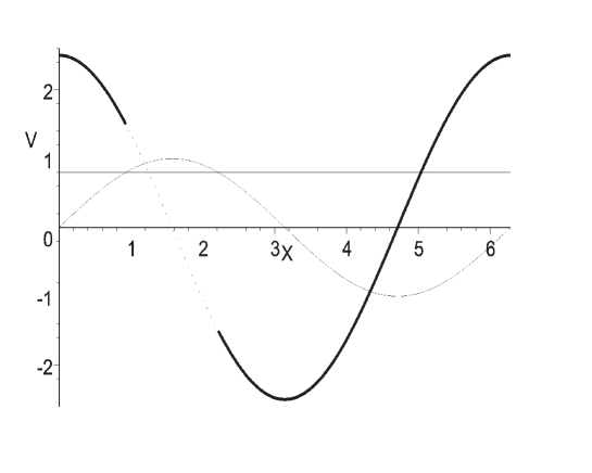
Figure 1: Trapping (medium solid line) and forbidden (dotted line) regions of the grazing manifold $V=\lambda\cos X$; $V=\frac{2}{\lambda}$ and $V=\sin X$ (thin solid lines),$\ \lambda=2.5$. Critical points are at the ends of dotted lines.

4.2 Impact oscillator

In the present Subsection we shall work in a general setting, proposed by Nordmark [16]. The equation of motion is:

$$\frac{d^{2}x}{dt^{2}}=A\left(x,\frac{dx}{dt},t\right),$$ (46)

with periodic acceleration function:

$$A\left(x,\frac{dx}{dt},t+2\pi\right)=A\left(x,\frac{dx}{dt},t\right).$$ (47)

The motion of the material point is confined to $x\geq x_{c}$ and the stationary impact boundary is given by $x=x_{c}$. The impact law is of form $v_{i+1}=G\left(v_{i}\right)$, $G\left(0\right)=0$, see for example Eq.( 3b). This equation of motion can describe linear impact oscillators as well as a ball bouncing on a vibrating table, see Section $5.2.3$ of [38] for the transformation relating systems with a moving boundary to systems with a stationary stop.

The solution of (46) can be written in form:

$$x=x\left(t,x_{c},v_{0},t_{0}\right),$$ (48)

with initial conditions $x\left(t_{0},x_{c},v_{0},t_{0}\right)=x_{c}$, $\left.\frac{dx\left(t,x_{c},v_{0},t_{0}\right)}{dt}\right|_{t=t_{0}^{+}}=v_{0}\geq 0$, i.e. we assume that the impact occurred at $t=t_{0}$. Let us also assume that the next impact occurs at $t=t_{1}$:

$$F\left(t_{1},x_{c},v_{0},t_{0}\right)\overset{df}{=}x\left(t_{1},x_{c},v_{0},t_{0}\right)-x_{c}=0,$$ (49)

where the time of the second impact is defined by (49) as an implicit function $t_{1}=f\left(x_{c},v_{0},t_{0}\right)$. Obviously, due to the initial condition, it follows that $t_{1}=t_{0}$ is the trivial solution of (49) and can be thus ignored. We shall next assume that $t_{1}-t_{0}$ is small - this assumption is clearly fulfilled in the phase of grazing. Expanding the function $F$ we get:

$$x_{c}+\left(t_{1}-t_{0}\right)\left.\frac{dx}{dt_{1}}\right|_{t=t_{0}^{+}}+\tfrac{1}{2}\left(t_{1}-t_{0}\right)^{2}\left.\frac{d^{2}x}{dt_{1}^{2}}\right|_{t=t_{0}^{+}}+O\left(\left(t_{1}-t_{0}\right)^{3}\right)-x_{c}=0.$$ (50)

Neglecting the trivial solution $t_{1}=t_{0}$ we obtain from (50 ) the approximate formula for the time interval elapsing between two subsequent impacts:

$$t_{1}-t_{0}=\frac{-2v_{0}}{A_{0}},$$ (51)

where $A_{0}\equiv\left.\frac{d^{2}x}{dt_{1}^{2}}\right|_{t=t_{0}^{+}}=A\left(x_{c},v_{0},t_{0}^{+}\right)$.

5 Basins of attraction

We have studied dependence of the dynamics on the control parameters. The bifurcation diagram is shown in Fig. $2$ for $R=0.85$ and $0\leq\lambda\leq 2.5$. It can be seen that for $\lambda<\lambda_{cr_{1}}^{\left(1\right)}=0.5094474\ldots\$only the grazing dynamics is possible. For $\lambda>\lambda_{cr_{1}}^{\left(1\right)}$ the first fixed point $P_{s}^{\left(1\right)}$ exists and is attractive and the second fixed point $P_{s}^{\left(2\right)}$ exists and is attractive for $\lambda>\lambda_{cr_{1}}^{\left(2\right)}=1.0188949\ldots\$. The first of $3$ - cycles, which typically accompany $1$ - cycles, appears for $\lambda\cong 1.78$ while several small attractors can be seen for $\lambda>1.5$.

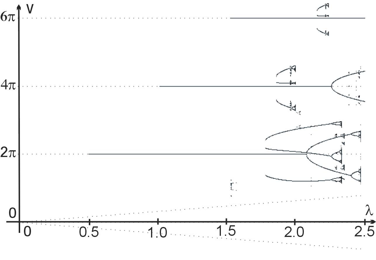
Figure 2: Bifurcation diagram, $R=0.85,\ 0\leq\lambda\leq 2.5$. Dotted lines enclose triangular region of grazing dynamics with $-\lambda\leq V\leq\lambda$.

It follows that for $\lambda_{cr_{1}}^{\left(1\right)}<\lambda<\lambda_{cr_{1}}^{\left(2\right)}$ there are two coexisting attractors only: the grazing manifold and the first fixed point $P_{s}^{\left(1\right)}$ .

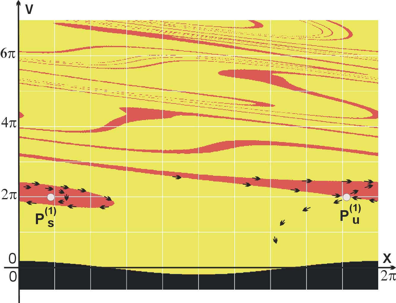
Figure 3: Basins of attraction, $R=0.85,\ \lambda=0.6$.

Basins of attraction of these two attractors are shown in Fig.$\,3$ above for $R=0.85,\ \lambda=0.6$. In the Figures $3-5$ basins of grazing dynamics are yellow, basins of $P_{s}^{\left(1\right)}$ are coloured red and basin of $P_{s}^{\left(2\right)}$ is green. Arrows denote direction of motion on stable and unstable manifolds of unstable fixed points $P_{u}^{\left(1\right)}$, $P_{u}^{\left(2\right)}$. Boundaries of the attractor’s basins are determined by the nature of the unstable fixed point $P_{u}^{\left(1\right)}$. This unstable fixed point appears for growing $\lambda$ when $\lambda\geq\lambda_{cr_{1}}^{\left(1\right)}\equiv\frac{2\pi(1-R)}{1+R}$. We have demonstrated in Section $3$ that eigenvalues of the characteristic equation fulfill inequalities $0\leq\Lambda_{1}<1$ and$\ 1<\Lambda_{2}$ $\left(\lambda>\lambda_{cr_{1}}^{\left(1\right)}\right)$. Therefore the fixed point $P_{u}^{\left(1\right)}$ is a saddle: it has one-dimensional unstable manifold $W_{u}\left(P_{u}^{\left(1\right)}\right)\$as well as one-dimensional stable manifold $W_{s}\left(P_{u}^{\left(1\right)}\right)\$in the phase space $\left(X,\ V\right)$. The basin boundary is exactly the manifold $W_{s}\left(P_{u}^{\left(1\right)}\right)\$[39].

We can see in Fig. 3 fractalization of the basins for large velocities. This phenomenon is enhanced for larger values of $\lambda$, see Fig. $4$ below.

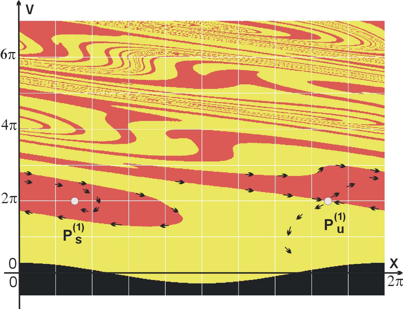
Figure 4: Basins of attraction, $R=0.85,\ \lambda=0.9$.

For higher values of $\lambda$, $\lambda\geq\lambda_{cr_{1}}^{\left(2\right)}\equiv\tfrac{4\pi(1-R)}{1+R}$, the second pair of $1$ - cycles, $P_{s}^{\left(2\right)}$ and $P_{u}^{\left(2\right)}$, exist (the first attractive and the second one a saddle). Basin boundaries are formed by $W_{s}\left(P_{u}^{\left(1\right)}\right)$ and $W_{s}\left(P_{u}^{\left(2\right)}\right)$, see Fig. $5$.

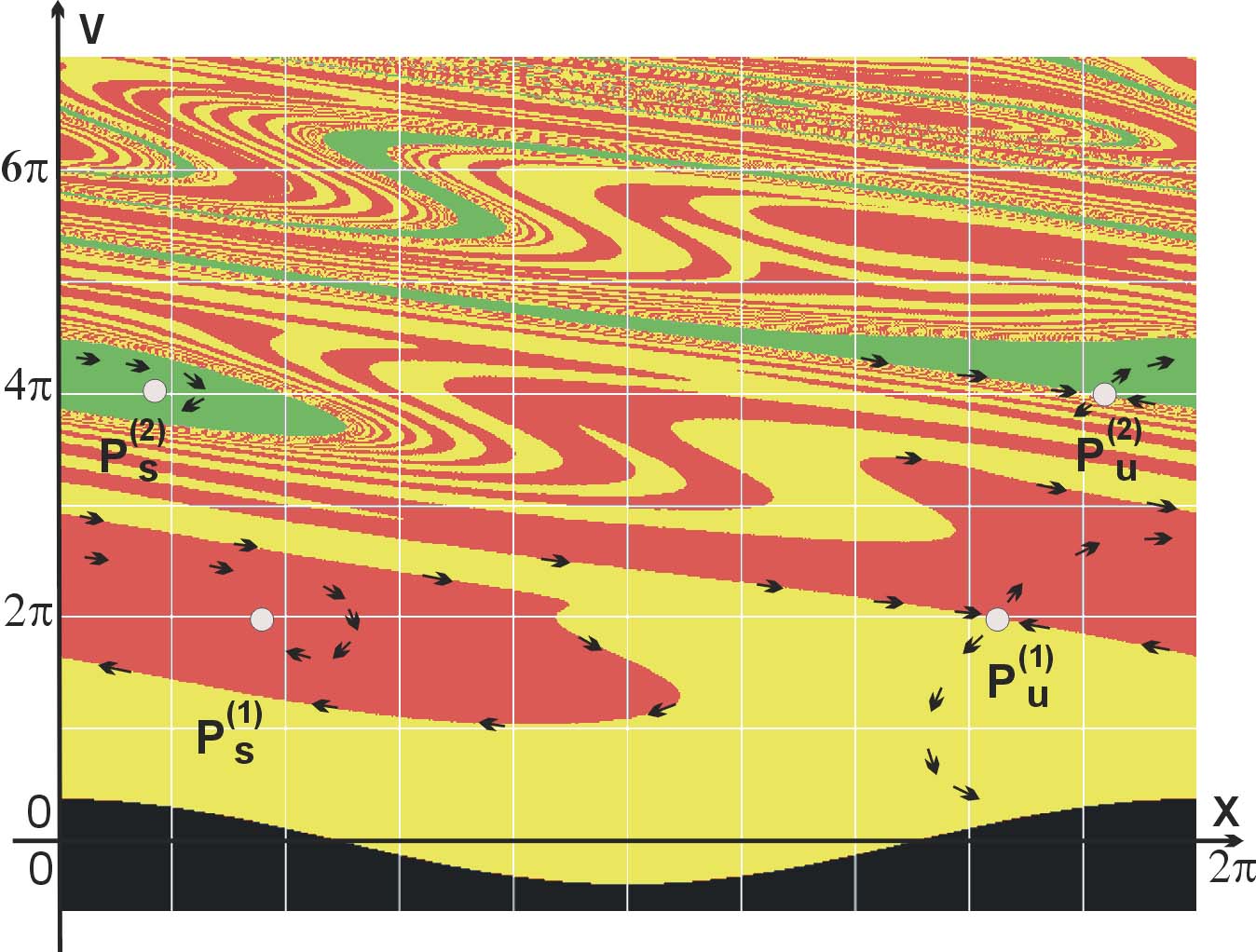
Figure 5: Basins of attraction, $R=0.85,\ \lambda=1.2$.

In Figs. $3,\ 4,\ 5$ fractalization of the basins of attraction is clearly seen. In other words, the manifolds $W_{s}\left(P_{u}^{\left(1\right)}\right)$, $W_{s}\left(P_{u}^{\left(2\right)}\right)$, which contribute to the basins boundaries, become fragmented or shredded. The shredding process of the manifolds was predicted and qualitatively described by Whiston [15]. It also seems that all three basins in Fig. $5$ are intermingled in some parts of the phase space.

6 Discussion

We have analyzed dynamics of the bouncing ball via the Poincaré map. We have found approximate solution, (39), of Eq.(17a) defining time of the next impact as the implicit function, $X_{i+1}=f\left(X_{i},\ V_{i}\right)$, near the grazing manifold, except from some critical points, discussed below. It was possible to determine approximate form of the implicit function because the series expansion of (17a) converges near the grazing manifold, moreover the trivial solution, $X_{i+1}=X_{i}$, was recognized as an initial condition and was eliminated, accordingly. The solution (39) or (40) was shown be valid for more general impacting systems, see Eq.(51). The critical points on the grazing manifold turn out to be zeroes of the post-impact acceleration. Let us note here that importance of the acceleration function was stressed by Whiston and Nordmark [14, 15, 16].

We have also studied dependence on initial conditions for the map (17) in the case of coexisting attractors, namely grazing dynamics and the first fixed point $P_{s}^{\left(1\right)}$, as well as the second fixed point $P_{s}^{\left(2\right)}$. It is interesting that for initial conditions with large velocities fractalization of basins boundaries can be observed. This effect was predicted by Whiston [15].

There are several possible directions for further investigations. Firstly, the role of critical points on the grazing manifold should be studied. Secondly, the shredding process, leading to fragmentation of basins of attraction, should be understood in detail. Finally, more general case of impacts can be considered. Namely, it is well known from experiments as well as from theoretical investigations that the coefficient of restitution depends on the impact velocity, $R=r\left(\dot{x}\right)$ [40, 33]. There were several experimental as well as theoretical attempts to determine dependence of the coefficient of restitution on impact velocity, see for example [41, 42] . It is thus possible to use the approach described in the present work in the case of velocity dependent coefficient of restitution, substituting in the impact equation (3b) the constant $R$ by a function $r\left(\dot{x}\right)$. Alternatively, continuous model of low-speed collisions can be considered [43].

References

- [1] di Bernardo, M., Budd, C.J., Champneys, A.R., Kowalczyk, P.: Bifurcations and Chaos in Piecewise Smooth Dynamical Systems. Theory and Applications. Springer (2006).
- [2] Feigin, M.I.: Period-doubling at C-bifurcations in piecewise continuous system. Pricladnaya Matemat. Mekh. 34, 861-869 (1970).
- [3] Feigin, M.I.: On subperiodic motions arising in the piecewise continuous systems. Pricladnaya Matemat. Mekh. 38, 810-818 (1974).
- [4] Feigin, M.I.: On the behaviour of dynamical systems near the boundary of existence region of periodic motions. . Pricladnaya Matemat. Mekh. 41, 628-636 (1977).
- [5] di Bernardo, M., Feigin, M.I., Hogan, S.J., Homer, M.E.: Local Analysis of C-Bifurcations in Dimensional Piecewise-Smooth Dynamical Systems. Chaos, Solitons and Fractals 10, 1881-1908 (1999).
- [6] Peterka, F.: Part 1: Theoretical analysis of - multiple - impact solutions. CSAV Acta Technica 19, 462-473 (1974).
- [7] Peterka, F.: Part 2: Results of analogue computer modelling of the motion. CSAV Acta Technica 19, 569-580 (1974).
- [8] Peterka, F., Vacik, J.: Transition to Chaotic Motion in Mechanical Systems with Impacts. J. Sound and Vibration 154, 95-115 (1992).
- [9] Shaw, S.W., Holmes, P.J.: Periodically forced linear oscillator with impacts: chaos and long-periodic motions. Phys. Rev. Lett. 51, 623-626 (1983).
- [10] Shaw, S.W., Holmes, P.J.: A periodically forced piecewise linear oscillator. J. Sound and Vibration 90, 129-144 (1983).
- [11] Shaw, S.W., Holmes, P.J.: A Periodically Forced Impact Oscillator with Large Dissipation. J. Appl. Mechanics 50, 849-857 (1983).
- [12] Thompson, J.M.T., Ghaffari, R.: Chaotic dynamics of an impact oscillator. Phys. Rev A 27, 1741-1743 (1983).
- [13] Thompson, J.M.T., Stewart, H.B.: Non-linear Dynamics and Chaos, John Wiley, New York (1986), Chapter 15: Chaotic motions of an impacting system.
- [14] Whiston, G.S.: Global dynamics of a vibro-impacting linear oscillator. J. Sound and Vibration 118, 395-429 (1987).
- [15] Whiston, G.S.: Singularities in vibro-impact dynamics. J. Sound and Vibration 152, 427-460 (1992).
- [16] Nordmark, A.B.: Non-periodic motion caused by grazing incidence in an impact oscillator. J. Sound and Vibration 145, 279-297 (1991).
- [17] A.B. Nordmark: Grazing conditions and chaos in impacting systems, PhD thesis, Royal Institute of Technology, Stockholm, Sweden (1992).
- [18] Nordmark, A.B.: Existence of periodic orbits in grazing bifurcations of impacting mechanical oscillator. Nonlinearity 14, 1517-1542 (2001).
- [19] Foale, S., Bishop, S.R.: Dynamical complexities of forced impacting systems. Phil. Trans. R. Soc. Lond. A 338, 547-556 (1992).
- [20] Foale, S., Bishop, S.R.: Bifurcations in impact oscillators. Nonlinear Dynam. 6, 285-289 (1994).
- [21] Fermi, E.: On the Origin of the Cosmic Radiation. Phys. Rev. 75, 1169-1174 (1949).
- [22] Ulam, S.: On some statistical properties of dynamical systems. In: Le Cam, M.L., Neyman, J., Scott, E. (eds.) Proceedings of Fourth Berkeley Symp. on Math. Stat. and Prob., vol. 3, p. 315. University of California Press 1961.
- [23] Brahic, A.: Numerical study of a simple dynamical system. Astron. and Astrophys. 12, 98-110 (1971).
- [24] Lieberman, M., Lichtenberg, A.J.: Stochastic and Adiabatic Behavior of Particles Accelerated by Periodic Forces. Phys. Rev. A 5, 1852-1866 (1972).
- [25] Lichtenberg, A.J., Lieberman, M., Cohen, R.H.: Fermi Acceleration Revisited. Physica D 1, 291-305 (1980).
- [26] Lichtenberg, A.J., Lieberman, M.: Regular and stochastic motion. Springer-Verlag, New York (1983).
- [27] Pustyl’nikov, L.D.: Stable and oscillating motions in nonautonomous dynamical systems. II. Moscow. Math. Soc. 34, 1-101 (1977).
- [28] Pustyl’nikov, L.D.: A new mechanism for particle acceleration and a relativistic analogue of the Fermi-Ulam model. Theoret. and Math. Phys. 77, 1110-1115 (1988).
- [29] Holmes, P.J.: The dynamics of repeated impacts with a sinusoidally vibrating table. J. Sound and Vibration 84, 173-189 (1982).
- [30] Pierański, P., Małecki, J.: Noisy precursors and resonant properties of the period-doubling modes in a nonlinear dynamical system. Phys. Rev. A 34, 582-590 (1986).
- [31] Kowalik, Z.J., Franaszek, M., Pierański, P., Self-reanimating chaos in the bouncing-ball system. Phys. Rev. A 37, 4016-4022 (1988).
- [32] Luo, A.C.J., Han, R.P.S.: The dynamics of a bouncing ball with a sinusoidally vibrating table revisited. Nonlinear Dynamics 10, 1-18 (1996).
- [33] Goldsmith, W.: Impact: The Theory and Physical Behavior of Colliding Solids, Edward Arnold, London (1960).
- [34] Pfeiffer, F., Glocker, C.: Multibody Dynamics with Unilateral Contacts, Wiley, New York (1996).
- [35] Gajewski K., Radziszewski B., On the stability of impact systems, Bull.of the Polish Acad.of Sci., Techn. Sciences. Appl. Mechanics. 35, 183-189 (1987).
- [36] Mickens, R. E.: Difference equations: theory and applications, 2nd ed. van Nostrand Reinhold, New York (1990).
- [37] Spivak, M.: Calculus on Manifolds. W.A. Benjamin, Inc., Menlo Park, California (1965).
- [38] Lamba, H.: Chaotic, regular and unbounded behaviour in the elastic impact oscillator. Physica D 82, 117-135 (1995).
- [39] Ott, E.: Chaos in Dynamical Systems. Cambridge University Press (1994).
- [40] Hodkinson, E.: On the collision of imperfectly elastic bodies. Report of the Fourth Meeting of the British Association for the Advancement of Science. London (1983).
- [41] Brach, R.M.: Mechanical impact dynamics. Wiley, New York (1991).
- [42] Stronge, W.J.: Impact mechanics. Cambridge University Press, Cambridge (2000).
- [43] Ivanov, A.P.: Bifurcations in Impact Systems. Chaos, Solitons and Fractals 7, 1615-1634 (1996).