Bose-Einstein condensation and Superfluidity of magnetoexcitons in Graphene

Abstract

We propose experiments to observe Bose-Einstein condensation (BEC) and superfluidity of quasi-two-dimensional (2D) spatially indirect magnetoexcitons in bilayer graphene. The magnetic field $B$ is assumed strong. The energy spectrum of collective excitations, the sound spectrum as well as the effective magnetic mass of magnetoexcitons are presented in the strong magnetic field regime. The superfluid density $n_{S}$ and the temperature of the Kosterlitz-Thouless phase transition $T_{c}$ are shown to be increasing functions of the excitonic density $n$ but decreasing functions of $B$ and the interlayer separation $D$. Numerical results are presented from these calculations.

Indirect excitons in coupled quantum wells (CQWs) in the presence or absence of a magnetic field $B$ have been the subject of recent experimental investigations Snoke ; Butov ; Timofeev ; Eisenstein . These systems are of particular interest because of the possibility of Bose-Einstein condensation (BEC) and the superfluidity of indirect excitons formed from electron-hole pairs. These may result in persistent electrical currents in each QW or coherent optical properties and Josephson junction phenomena Lozovik ; Birman ; Littlewood ; Vignale_drag ; Berman . In high magnetic fields, two-dimensional (2D) excitons survive in a substantially wider temperature range, as the exciton binding energies increase with magnetic field Lerner ; Paquet ; Kallin ; Yoshioka ; Ruvinsky ; Ulloa ; Moskalenko .

In this Letter we propose a new physical realization of magnetoexcitonic BEC and superfluidity in bilayer graphene with spatially separated electrons and holes in high magnetic field. Recent technological advances have allowed the production of graphene, which is a 2D honeycomb lattice of carbon atoms that form the basic planar structure in graphite Novoselov1 ; Zhang1 Graphene has been attracting a great deal of experimental and theoretical attention because of unusual properties in its bandstructure Novoselov2 ; Zhang2 ; Nomura ; Jain . It is a gapless semiconductor with massless electrons and holes which have been described as Dirac-fermions DasSarma . Since there is no gap between the conduction and valence bands in graphene without magnetic field, the screening effects result in the absence of excitons in graphene in the absence of magnetic field. A strong magnetic field produces a gap since the energy spectrum becomes discrete formed by Landau levels. The gap reduces screening and leads to the formation of magnetoexcitons.

We consider two parallel graphene layers separated by an insulating slab of SiO₂. The electrons in one layer and holes in the other can be controlled as in the experiments with CQWsSnoke ; Butov ; Timofeev ; Eisenstein by laser pumping (far infrared in graphene). The spatial separation of electrons and holes in different graphene layers can be achieved by applying an external electric field. Furthermore, the spatially separated electrons and holes can be created by varying the chemical potential by using a bias voltage between two graphene layers or between two gates located near the corresponding graphene sheets. Indirect magnetoexcitons are bound states of spatially separated electrons and holes in an external magnetic field. The ratio of the external voltage $V_{ext}$ to the interlayer separation $D$ required to create spatially separated electrons and holes in graphene layers with the 2D density $n=10^{11}cm^{-2}$ is given by $V_{ext}/D=4\pi enD/\epsilon_{b}=4.021\times 10^{4}$ V/cm. Here, $-e$ is the electron charge and $\epsilon_{b}=4.5$ is the dielectric constant of SiO₂. Since the critical electric field $E_{cr}$ of the dielectric breakdown for SiO₂ is $E_{cr}\approx 10^{6}V/cm$, we conclude that the external electric field for the spatially separated electrons and holes is less than the critical electric field for dielectric breakdown in SiO₂.

A conserved quantity for an isolated electron-hole pair for graphene in magnetic field $B$ is the exciton magnetic momentum $\hat{\mathbf{P}}$ defined as

$$\hat{\mathbf{P}}=-i\hbar\nabla_{e}-i\hbar\nabla_{h}+\frac{e}{c}(\mathbf{A}_{e}-\mathbf{A}_{h})-\frac{e}{c}[\mathbf{B}\times(\mathbf{r}_{e}-\mathbf{r}_{h})]\$$ (1)

for the Dirac equationIyengar as for the Schrödinger equation Gorkov ; Lerner ; Kallin . Here, $\mathbf{r}_{e}$ and $\mathbf{r}_{h}$ are 2D coordinate vectors of an electron and hole, respectively, $\mathbf{A}_{e}$ and $\mathbf{A}_{h}$ are the corresponding vector potential of an electron and hole. The cylindrical gauge for vector potential is used with $\mathbf{A}_{e(h)}=1/2[\mathbf{B}\times\mathbf{r}_{e(h)}]$.

Neglecting transitions between Landau levels for high magnetic fields, we employ first-order perturbation theory to the Coulomb attraction $V(r)=-e^{2}/(\epsilon_{b}\sqrt{r^{2}+D^{2}})$ between an electron and hole. Here, $\mathbf{r}=\mathbf{r}_{e}-\mathbf{r}_{h}$. We calculate the magnetoexciton energy using the expectation value for an electron in Landau level $1$ and a hole in level $1$. We have

$$E_{1,1}(P)=\left\langle 0,0,\mathbf{P}\left|\hat{V}(r)\right|0,0,\mathbf{P}\right\rangle$$ (2)

$$+ \left\langle 0,1,\mathbf{P}\left|\hat{V}(r)\right|0,1,\mathbf{P}\right\rangle+\left\langle 0,1,\mathbf{P}\left|\hat{V}(r)\right|0,1,\mathbf{P}\right\rangle$$

$$+ \left\langle 1,0,\mathbf{P}\left|\hat{V}(r)\right|1,0,\mathbf{P}\right\rangle,$$

where $\left|\tilde{n},m,\mathbf{P}\right\rangle$ is an eigenfunction of the non-relativistic Hamiltonian of a non-interacting electron-hole pair defined in Lerner ; Ruvinsky . For small magnetic momentum satisfying $P\ll\hbar/r_{B}$ and $P\ll\hbar D/r_{B}^{2}$, we obtain the following relationsRuvinsky

$$\langle\langle\tilde{n}m\mathbf{P}|\hat{V}(r)|\tilde{n}m\mathbf{P}\rangle\rangle=\mathcal{E}_{\tilde{n}m}^{(b)}+\frac{P^{2}}{2M_{\tilde{n}m}(B,D)}\ .$$ (3)

Substituting these results into Eq. (2), we obtain the binding energy $\mathcal{E}_{B}^{(b)}(D)$ and the effective magnetic mass $m_{B}(D)$ of a magnetoexciton with spatially separated electron and hole in bilayer graphene as $\mathcal{E}_{B}^{(b)}(D)=\mathcal{E}_{00}^{(b)}(B,D)+2\mathcal{E}_{01}^{(b)}(B,D)+\mathcal{E}_{10}^{(b)}(B,D)$, and $m_{B}^{-1}(D)=M_{00}^{-1}(B,D)+M_{01}(B,D)^{-1}+M_{10}^{-1}(B,D)$, where constants $\mathcal{E}_{00}^{(b)}(B,D)$, $\mathcal{E}_{01}^{(b)}(B,D)$, $\mathcal{E}_{10}^{(b)}(B,D)$, $M_{00}(B,D)$, $M_{01}(B,D)$ and $M_{10}(B,D)$ depending on magnetic field $B$ and the interlayer separation $D$ in detail are given in  Ruvinsky :

$$\mathcal{E}_{00}^{(b)}(B,D) = -\mathcal{E}_{0}\exp\left[\frac{D^{2}}{2r_{B}^{2}}\right]\mathrm{erfc}\left[\frac{D}{\sqrt{2}r_{B}}\right],$$

$$M_{00}(B,D) = M_{0}\left[\left(1+\frac{D^{2}}{r_{B}^{2}}\right)\exp\left[\frac{D^{2}}{2r_{B}^{2}}\right]\mathrm{erfc}\left[\frac{D}{\sqrt{2}r_{B}}\right]\right.$$ (4)

$$- \left.\sqrt{\frac{2}{\pi}}\frac{D}{r_{B}}\right]^{-1}\ .$$

Here, $r_{B}=\sqrt{\hbar c/(eH)}$ is the magnetic length; $c$ is the speed of light, $\mathcal{E}_{0}=e^{2}/\epsilon_{b}r_{B}\sqrt{\pi/2}$, $M_{0}=2^{3/2}\hbar^{2}\epsilon_{b}/(\sqrt{\pi}e^{2}r_{B})$ and $\mathrm{erfc}(z)$ is the complementary error function Ruvinsky . The radius of a magnetoexciton in the lowest Landau level is given by $r_{1,1}(B)=4r_{B}$.

For large interlayer separation $D\gg r_{B}$, the asymptotic values of the binding energy $\mathcal{E}_{B}^{(b)}(D)$ and the effective magnetic mass $m_{B}(D)$ are $\mathcal{E}_{B}^{(b)}(B,D)=-4e^{2}/(\epsilon_{b}D)$, and $m_{B}(D)=\epsilon_{b}D^{3}B^{2}/(4c^{2})$. When $D\ll r_{B}$, these quantities denoted by $\mathcal{E}_{0}$ and $M_{0}$ are presented above. We can see that the effective magnetic mass of an indirect magnetoexciton is approximately four times smaller than in CQWs at the same $D$, $\epsilon_{b}$ and $\mathbf{B}$ Ruvinsky . The magnetoexcitonic energy is approximately four times larger in bilayer graphene than in CQWs. Measuring energies relative to the binding energy of a magnetoexciton, the dispersion relation $\varepsilon_{k}(P)$ of a magnetoexciton is quadratic at small magnetic momentum, i.e., $P\ll\hbar/r_{B}$ and $P\ll\hbar D/r_{B}^{2}$. We have $\varepsilon_{k}({\bf P})=P^{2}/(2m_{Bk})$, where $m_{Bk}$ is the effective magnetic mass, dependent on $B$, $D$ and the magnetoexcitonic quantum numbers $k=\{n_{+},n_{-}\}$ for an electron in Landau level $n_{+}$ and a hole in level $n_{-}$. Indirect magnetoexcitons, either in the ground state or an excited state, have electrical dipole moments. We treat these excitons as interacting parallel electric dipoles. This is valid when $D$ is larger than the mean separation $\langle r\rangle$ between an electron and hole parallel to the graphene layers. We take into account that at high magnetic fields $\langle r\rangle\approx Pr_{B}^{2}/\hbar$ with $\langle{\bf r}\rangle$ perpendicular to ${\bf P}$. Typical values of magnetic momenta are given by $P\sim\hbar\sqrt{n}$, where $n$ is the 2D density of magnetoexcitons for a parabolic dispersion relation. Consequently, $D\gg\langle r\rangle$ is valid when $D\gg\sqrt{n}r_{B}^{2}$. Since electrons on a graphene lattice can be in two valleys, there are four types of excitons in bilayer graphene. Due to the fact that all these types of excitons have identical envelope wave functions and energiesIyengar , we consider below only excitons in one valley. Also, we use $n_{0}=n/4$ as the density of excitons in one layer, with $n$ denoting the total density of excitons. For large electron-hole separation $D\gg r_{B}$, transitions between Landau levels due to the Coulomb electron-hole attraction can be neglected, if the following condition is valid, i.e., $E_{b}=4e^{2}/(\epsilon_{b}D)\ll\hbar v_{F}/r_{B}$. This corresponds to high magnetic field $B$, large interlayer separation $D$ and large dielectric constant of the insulator layer between the graphene layers. In this notation, $v_{F}=\sqrt{3}at/(2\hbar)$ is the Fermi velocity of electrons. Also, $a=2.566\AA$ is a lattice constant, $t\approx 2.71eV$ is the overlap integral between nearest carbon atoms Lukose .

The distinction between excitons and bosons is due to exchange effects Berman . These effects for excitons with spatially separated electrons and holes in a dilute system satisfying $na^{2}(B,D)\ll 1$ are suppressed due to the negligible overlap of the wave functions of two excitons as a result of the potential barrier, associated with the dipole-dipole repulsion Berman . Two indirect excitons in a dilute system interact via $U(R)=e^{2}D^{2}/(\epsilon_{b}R^{3})$, where $R$ is the distance between exciton dipoles along the graphene layers. In high magnetic fields, the small parameter mentioned above has the form $\exp[-2\hbar^{-1}(m_{Bk})^{1/2}eDa^{-1/2}(B,D)]$. So at $T=0$, the dilute gas of magnetoexcitons, which is a boson system, form a Bose condensate Griffin . Therefore, the system of indirect magnetoexcitons can be treated by the diagrammatic technique for a boson system. For the dilute 2D magnetoexciton system with $na^{2}(B,D)\ll 1$, the sum of ladder diagrams is adequate. For the lowest Landau level, we denote $\varepsilon_{11}({\bf P})=\varepsilon({\bf P})$. Using the orthonormality of the four-component wave functions of the relative coordinate for a non-interacting pair of an electron in Landau level $n_{+}$ and a hole in level $n_{-}$ ($\tilde{\Phi}_{n_{+},n_{-}}(\mathbf{P}=\mathbf{0},\mathbf{r})$)Iyengar we obtain an approximate equation for the vertex $\Gamma$ in strong magnetic fields. Due to the orthonormality of the four-component wave functions $\tilde{\Phi}_{n_{+},n_{-}}({\bf 0,r})$ the projection of the equation for the vertex in the ladder approximation for a dilute system onto the lowest Landau level results in the scalar integral equation which does not reflect the spinor nature of the four-component magnetoexcitonic wave functions in graphene. In high magnetic field, one can ignore transitions between Landau levels and consider only the lowest Landau level states $n_{+}=n_{-}=1$. Since typically, the value of $r$ is $r_{B}$, and $P\ll\hbar/r_{B}$ in this approximation, the equation for the vertex in the magnetic momentum representation $P$ for the lowest Landau level has the same form (compare with Lozovik ) as for a 2D boson system in the absence of magnetic field, but with the magnetoexciton magnetic mass $m_{B}$ (which depends on $B$ and $D$) instead of the exciton mass ($M=m_{e}+m_{B}$) and magnetic momentum instead of inertial momentum:

$$\Gamma(\mathbf{p},\mathbf{p}^{\prime};P)=U(\mathbf{p}-\mathbf{p}^{\prime})$$

$$+\int\frac{d^{2}q}{(2\pi\hbar)^{2}}\frac{U(\mathbf{p}-\mathbf{q})\Gamma(\mathbf{q},\mathbf{p}^{\prime};P)}{\frac{\kappa^{2}}{m_{B}}+\Omega-\frac{\mathbf{P}^{2}}{4m_{B}}-\frac{q^{2}}{m_{B}}+i\delta},\hskip 5.69046pt\delta\to 0^{+}$$

$$\mu = \frac{\kappa^{2}}{2m_{B}}=n_{0}\Gamma_{0}=n_{0}\Gamma(0,0;0)\ ,$$ (5)

where $P=\{\mathbf{P},\Omega\}$, and $\mu$ is the chemical potential of the system. Equation (5) is valid at parameter values which satisfy the condition for validity of the perturbation theory applied to the calculation of the magnetoexcitonic binding energy. The specific feature of a 2D Bose system is connected with a logarithmic divergence in the 2D scattering amplitude at zero energy Lozovik ; Berman . A simple analytical solution of Eq. (5) for the chemical potential can be obtained if $\kappa m_{B}e^{2}D^{2}/(\hbar^{3}\epsilon)\ll 1$. In strong magnetic fields at $D\gg r_{B}$ the exciton magnetic mass is defined as $m_{B}\approx\hbar^{2}\epsilon D^{3}/(4e^{2}r_{B}^{4})$. So the inequality $\kappa m_{B}e^{2}D^{2}/(\hbar^{3}\epsilon)\ll 1$ is valid if $D\ll(r_{B}^{4}/n^{1/2})^{1/5}$. Consequently, the chemical potential $\mu$ is obtained as

$$\mu=\frac{\kappa^{2}}{2m_{B}}=\frac{8\pi\hbar^{2}n}{8m_{B}\log\left[\hbar^{4}\epsilon^{2}/\left(2\pi nm_{B}^{2}e^{4}D^{4}\right)\right]}.$$ (6)

At small magnetic momentum, the solution of Eq.(5) corresponds to the sound spectrum of collective excitations $\varepsilon(P)=c_{s}P$. Here, the sound velocity $c_{s}=\sqrt{\Gamma n/(4m_{B})}=\sqrt{\mu/m_{B}}$, where $\mu$ is guven by Eq. (6). Since magnetoexcitons have a sound spectrum of collective excitations at small magnetic momentum $P$ due to the dipole-dipole repulsion, the magnetoexcitonic superfluidity is possible at low temperature $T$ in bilayer graphene. This is so since the sound spectrum satisfies the Landau criterium of superfluidity Griffin .

It can be shown that when $D=0$, the interaction between two magnetoexcitons in the lowest Landau level can be neglected in strong magnetic field Lerner . The magnetoexcitons constructed by spatially separated electrons and holes in bilayer graphene at large interlayer separations $D\gg r_{B}$ form a weakly interacting 2D non-ideal Bose gas with a dipole-dipole repulsion. Thus, the phase transition from the normal to superfluid phase is the Kosterlitz-Thouless transition Kosterlitz . The temperature of this phase transition $T_{c}$ to the superfluid state in a 2D magnetoexciton system is determined from $T_{c}=\pi\hbar^{2}n_{S}(T_{c})/(2k_{B}m_{B})$, where $n_{S}(T)$ is the superfluid density of the magnetoexciton system, as a function of $T$, $B$, $D$ and $k_{B}$ is Boltzmann’s constant. The function $n_{S}(T)$ can be obtained from $n_{S}=n/4-n_{n}$, with $n$ the total density and $n_{N}$ the normal component density. To calculate the superfluid component density, we find the total quasiparticle current in a reference frame in which the superfluid component is at rest. We determine the normal component density by the usual procedure Griffin . Suppose that the magnetoexciton system moves with a velocity $\mathbf{u}$. At nonzero temperatures dissipating quasiparticles will appear in this system. Since their density is small at low temperatures, one can assume that the gas of quasiparticles is an ideal Bose gas. To calculate the superfluid component density, we find the total current of quasiparticles in a frame of reference in which the superfluid component is at rest. We denote $\langle Pk|...|Pk\rangle$ as $\langle\cdots\rangle$. Using the Feynman theorem for isolated magnetoexcitons, we obtain the velocity Gorkov $\mathbf{v}=\left\langle\hat{\mathbf{v}}\right\rangle=\left\langle\partial\hat{H}/\partial\mathbf{P}\right\rangle=\partial\varepsilon_{k}(P)/\partial\mathbf{P}=\mathbf{P}/m_{Bk}$. We obtain the mean total current of 2D magnetoexcitons in the coordinate system, moving with a velocity ${\bf u}$ as $\left\langle\mathbf{J}\right\rangle=\left\langle\mathbf{P}\right\rangle/m_{B}$. Expanding the integrand to first order by $\mathbf{P}\mathbf{u}/(k_{B}T)$, we have

$$\langle\mathbf{J}\rangle = -\frac{\mathbf{u}}{2m_{B}}\int\frac{d\mathbf{P}}{(2\pi\hbar)^{2}}P^{2}\frac{\partial f\left[\varepsilon(P)\right]}{\partial\varepsilon}$$ (7)

$$= \frac{3\zeta(3)}{2\pi\hbar^{2}}\frac{k_{B}^{3}T^{3}}{m_{B}c_{s}^{4}}\mathbf{u}\ ,$$

where $f\left[\varepsilon(P)\right]=\left(\exp\left[\varepsilon(P)/(k_{B}T)\right]-1\right)^{-1}$ is the Bose-Einstein distribution function and $\zeta(z)$ is the Riemann zeta function ($\zeta(3)\simeq 1.202$). Then we define the normal component density isGriffin $\langle\mathbf{J}\rangle=n_{n}\mathbf{u}$. Applying Eq. (7), we obtain the expression for the normal density $n_{N}$. As a result, we have for the superfluid density: $n_{S}(T)=n/4-n_{N}(T)$. It follows that the expression for the superfluid density $n_{S}$ in strong magnetic field for the proposed magnetoexciton system differs from the analogous expression in the absence of magnetic field in semiconductor CQWs (compare with Refs. Berman ) by replacing the total exciton mass $M=m_{e}+m_{B}$ with the magnetoexciton magnetic mass $m_{B}$.

In a 2D system, superfluidity of magnetoexcitons appears below the Kosterlitz-Thouless transition temperature, where only coupled vortices are present Kosterlitz . Employing $n_{S}(T)$ for the superfluid component, we obtain an equation for the Kosterlitz-Thouless transition temperature $T_{c}$ with solution

$$T_{c}=\left[\left(1+\sqrt{\frac{32}{27}\left(\frac{4m_{B}k_{B}T_{c}^{0}}{\pi\hbar^{2}n}\right)^{3}+1}\right)^{1/3}\right.$$

$$-\left.\left(\sqrt{\frac{32}{27}\left(\frac{4m_{B}k_{B}T_{c}^{0}}{\pi\hbar^{2}n}\right)^{3}+1}-1\right)^{1/3}\right]\frac{T_{c}^{0}}{2^{1/3}}\ .$$ (8)

Here, $T_{c}^{0}$ is an auxiliary quantity, equal to the temperature at which the superfluid density vanishes in the mean-field approximation, i.e., $n_{S}(T_{c}^{0})=0$, $T_{c}^{0}=k_{B}^{-1}\left(2\pi\hbar^{2}nc_{s}^{4}m_{B}/(12\zeta(3))\right)^{1/3}$. The temperature $T_{c}^{0}=T_{c}^{0}(B,D)$ may be used to estimate the crossover region where local superfluid density appearers for magnetoexcitons on a scale smaller or of the order of the mean intervortex separation in the system. The local superfluid density can manifest itself in local optical or transport properties. The dependence of $T_{c}$ on $B$ and $D$ is represented in Fig. 1. According to Eq. (8), the temperature $T_{c}$ for the onset of superfluidity due to the Kosterlitz-Thouless transition at a fixed magnetoexciton density decreases as a function of magnetic field $B$ and interlayer separation $D$. This is due to the increased $m_{B}$ as a functions of $B$ and $D$. The $T_{c}$ decreases as $B^{-{1}/{2}}$ at $D\ll r_{B}$ or as $B^{-2}$ when $D\gg r_{B}$.

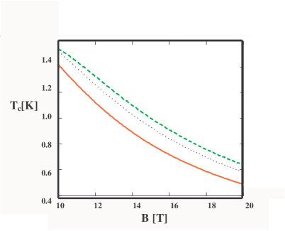
Figure 1: (Color on line) Dependence of Kosterlitz-Thouless transition temperature $T_{c}=T_{c}(B)$ (in units $K$) versus magnetic field for bilayer graphene separated by SiO₂. with $\epsilon_{b}=4.5$. The magnetoexciton density $n=4\times 10^{11}cm^{-2}$. Different interlayer separations $D$ are chosen: $D=30nm$ (solid curve), $D=28nm$ (dotted curve), $D=27nm$ (dashed curve).

In conclusion, we have studied BEC and superfluidity of magnetoexcitons in two graphene layers with applied external voltage in perpendicular magnetic field. The superfluid density $n_{S}(T)$ and the temperature of the Kosterlitz-Thouless phase transition to the superfluid state have been calculated. We have shown that at fixed exciton density $n$ the Kosterlitz-Thouless temperature $T_{c}$ for the onset of superfluidity of magnetoexcitons decreases as a function of magnetic field like $B^{-1/2}$ at $D\lesssim r_{B}$ and as $B^{-2}$ when $D\gg r_{B}$. We have shown that $T_{c}$ increases when the density $n$ increases and decreases when the magnetic field $B$ and the interlayer separation increase. The dependence of $T_{c}$ on $B$ and $D$ is presented in Fig. 1. We also note that the superfluidity of indirect magnetoexcitons in strong perpendicular magnetic field in bilayer graphene is very interesting, because the magnetoexcitons in graphene are found to be more stable than in CQWs. Namely, the binding energy of magnetoexcitons in graphene is four times greater than that in CQWs with the same $D$, $\epsilon_{b}$ and $\mathbf{B}$. We consider only the collective properties of excitons with electrons and holes from the same valley. We note that there is no crossover between Bose condensates of different types of excitons.

- (1) D. W. Snoke, Science 298, 1368 (2002).
- (2) L. V. Butov, J. Phys.: Condens. Matter 16, R1577 (2004).
- (3) V. B. Timofeev and A. V. Gorbunov, J. Appl. Phys. 101, 081708 (2007).
- (4) J. P. Eisenstein and A. H. MacDonald, Nature 432, 691 (2004).
- (5) Yu. E. Lozovik and V. I. Yudson, JETP Lett. 22, 26(1975); JETP 44, 389 (1976); Physica A 93, 493 (1978).
- (6) J. Zang, D. Schmeltzer and J. L. Birman, Phys. Rev. Lett. 71, 773 (1993).
- (7) X. Zhu, P. Littlewood, M. Hybertsen and T. Rice, Phys. Rev. Lett. 74, 1633 (1995).
- (8) G. Vignale and A. H. MacDonald, Phys. Rev. Lett. 76 2786 (1996).
- (9) Yu. E. Lozovik and O. L. Berman, JETP Lett. 64, 573 (1996); JETP 84, 1027 (1997); Yu. E. Lozovik, O. L. Berman, and M. Willander, J. Phys.: Condens. Matter 14, 12457 (2002).
- (10) I. V. Lerner and Yu. E. Lozovik, JETP 51, 588 (1980); JETP, 53, 763 (1981); A. B. Dzyubenko and Yu. E. Lozovik, J. Phys. A 24, 415 (1991).
- (11) D. Paquet, T. M. Rice, and K. Ueda, Phys. Rev. B32, 5208 (1985).
- (12) C. Kallin and B. I. Halperin, Phys. Rev. B30, 5655 (1984); Phys. Rev. B31, 3635 (1985).
- (13) D. Yoshioka and A. H. MacDonald, J. Phys. Soc. Jpn 59, 4211 (1990).
- (14) Yu. E. Lozovik and A. M. Ruvinsky, Phys. Lett. A 227, 271 (1997); JETP 85, 979 (1997).
- (15) M. A. Olivares-Robles and S. E. Ulloa, Phys. Rev. B64, 115302 (2001).
- (16) S. A. Moskalenko, M. A. Liberman, D. W. Snoke and V. V. Botan, Phys. Rev. B66, 245316 (2002).
- (17) K. S. Novoselov et al., Science 306, 666 (2004).
- (18) Y. Zhang, J. P. Small, M. E. S. Amori and P. Kim, Phys. Rev. Lett. 94, 176803 (2005).
- (19) K. S. Novoselov et al., Nature (London) 438, 197 (2005).
- (20) Y. B. Zhang et al., Nature (London) 438, 201 (2005).
- (21) K. Nomura and A. H. MacDonald, Phys. Rev. Lett. 96, 256602 (2006).
- (22) C. Tőke, P. E. Lammert, V. H. Crespi, and J. K. Jain, Phys. Rev. B74, 235417 (2006).
- (23) S. Das Sarma, E. H. Hwang, and W.- K. Tse, Phys. Rev. B75, 121406(R) (2007).
- (24) A. Iyengar, Jianhui Wang, H. A. Fertig, and L. Brey, Phys. Rev. B75, 125430 (2007).
- (25) L. P. Gorkov and I. E. Dzyaloshinskii, JETP 26, 449 (1967).
- (26) V. Lukose, R. Shankar, and G. Baskaran, Phys. Rev. Lett. 98, 116802 (2007).
- (27) A. Griffin, Excitations in a Bose-Condensed Liquid (Cambridge University Press, Cambridge, England, 1993).
- (28) J. M. Kosterlitz and D. J. Thouless, J. Phys. C 6, 1181 (1973); D. R.Nelson and J. M. Kosterlitz, Phys. Rev. Lett. 39, 1201 (1977).