Diagnostic tools for 3D unstructured oceanographic data

Abstract

Most ocean models in current use are built upon structured meshes. It follows that most existing tools for extracting diagnostic quantities (volume and surface integrals, for example) from ocean model output are constructed using techniques and software tools which assume structured meshes. The greater complexity inherent in unstructured meshes (especially fully unstructured grids which are unstructured in the vertical as well as the horizontal direction) has left some oceanographers, accustomed to traditional methods, unclear on how to calculate diagnostics on these meshes. In this paper we show that tools for extracting diagnostic data from the new generation of unstructured ocean models can be constructed with relative ease using open source software. Higher level languages such as Python, in conjunction with packages such as NumPy, SciPy, VTK and MayaVi, provide many of the high-level primitives needed to perform 3D visualisation and evaluate diagnostic quantities, e.g. density fluxes. We demonstrate this in the particular case of calculating flux of vector fields through isosurfaces, using flow data obtained from the unstructured mesh finite element ocean code ICOM, however this tool can be applied to model output from any unstructured grid ocean code.

, ,

1 Introduction

The development of an ocean model poses a broad range of challenges (in addition to the key challenges posed by validation against real world circulation and hydrography). Challenges involving the core of a model include the design of discretisation schemes, issues of numerical stability, good representation of hydrostatic and geostrophic balance, data I/O, time varying boundary forcing and relaxation to climatology, scalability for parallel computation etc. In addition to this, models are generally viewed as requiring a pre-processor for model preparation (e.g. mesh generation, setting model parameters and boundary conditions), and a post-processor for the analysis of model results. Because of their maturity, there has been a level of convergence of technologies and standards for structured grid ocean models. For example, and the subject of this paper, the ocean modelling community has amassed a wealth of methods and tools for the analysis of model results: Ncview provides a quick and easy way to browse data conforming to the NetCDF Climate and Forecast (CF) Metadata Convention; Ferret is a powerful visualization and analysis environment for large and complex gridded data sets, supporting numerous gridded file formats and standards including OPeNDAP (Open-source Project for a Network Data Access Protocol); MATLAB is also widely used since it combines easily accessible linear algebra routines together with interactive graphical output. However, file formats and standards for unstructured grid models are only emerging within the oceanographic community. For example, only recently has the community outlined what a standard might be and a set of milestones for implementation (Aikman et al. (2006)). Inevitably, application programming interfaces (APIs) for these emerging standards are still some way off. This in itself is an important consideration for researchers interested in developing software tools for analysing the output of unstructured ocean mesh models since there is a risk that software developed will rapidly become redundant. In addition, the actual data is more complex: for example, interpolating a single point within an unstructured data set is much more expensive (and complex if performed efficiently) than with a simple gridded data set which has in general an implicit spatial-temporal index.

Fortunately, there is a rich selection of open source tools which facilitates the design and development of diagnostics for complex diagnostics on unstructured grids. Diagnostic tools must be effective and relatively cheap to create (read scientist sweat-and-tears) as the underlying technology is evolving rapidly and tools are likely to have a short shelf life. Here we will consider the use of Python (a portable interrupted language) which has risen to prominence in science and engineering in recent years, particularly due to the addition of libraries such as NumPy and SciPy (Oliphant, 2007). The Visualization ToolKit (VTK) is another open source project which provides a Python API (also provides an API for C++, Java and TCL/TK), thus enabling a rich environment for creating 3D OpenGL scientific visualisation. This API provides ample functionality to perform differentiation, integration and interpolation on structured grids and unstructured grids containing linear tetrahedra, hexahedra, triangular prisms (wedges), pyramids and quadratic tethahedra and hexahedra elements as well as linear and quadratic triangles and quadrilaterals. The wedge elements are used by many ocean models which are unstructured in the horizontal but structured in the vertical: this includes SUNTANS (Stanford) which is a finite volume code, and SLIM (Louvain-la-Neuve) which uses nonconforming and discontinuous linear elements. FEOM (Bremerhaven) uses continuous linear tetrahedral elements (with wedge elements under development). ICOM (Imperial College London) uses tetrahedral and hexahedral elements. Multilayered 2D shallow-water models such as Delfin (Delft) and ADCIRC (Notre Dame) could also make use of this framework.

The reason that we choose the VTK/Mayavi combination is that the Python model of development, in which the developer time is considered at a premium with optimisation taking place only where it is necessary, facilates quick development of new tools in a rapidly changing scientific environment. Additionally, these projects have open source licenses which facilitates cross-project collaboration and comparison between models.

To illustrate what is involved in creating new and novel diagnostics for data on unstructured meshes, we extend the open source visualisation package MayaVi (Ramachandran, 2001), which is developed using Python and VTK. Importantly, diagnostics constructed in the manner can be applied to both structured and unstructured data sets; the only effort being to write code to convert from the data format to a VTK file (which can be done using the VTK API). This is crucial both to the portability of the methods and to comparisons of results from different models.

The motivating example developed here is the case of fluxes through isosurfaces since they are among the most complicated diagnostic quantities to calculate and visualise. The filter that we discuss has been added to the Mayavi source trunk and is freely available. It can be applied to output from any of the unstructured grid models described above (as well as structured grid models).

In Section 2, we describe the general methodology of using VTK and MayaVi, with reference to the isosurface case as an example. In Section 3, we show diagnostics calculated from ICOM output data: namely, temperature fluxes through vertical levels and volume flux through temperature isosurfaces calculated from a deep convection test case. Section 4 provides a summary and outlook.

2 Methodology

A finite element representation defines field values everywhere in the domain, not just at the grid points. This means that it is possible to define isosurfaces and integrals uniquely with respect to that representation; it is also possible to monitor the values of fields at any location as the solution evolves in time. If the finite element representation used is piecewise-linear or piecewise-quadratic then these calculations can all be performed within the VTK framework.

The VTK API readily facilitates a pipeline programming paradigm. Operations (such as the contour filter used in the following section) are performed by creating objects which require a reference to an input data set and provide a reference to an output data set, which itself may be passed as input to another operation. This means that when a property changes further up the pipeline, e.g. a different field value is chosen for an isosurface filter, that change is propagated all the way along the chain. This makes applications developed in this way very interactive: ideal for scientific analysis of data.

In MayaVi, operations are divided conceptually into modules and filters. Modules are used to obtain some mode of graphical representation of the data e.g. isosurfaces, flow vectors, streamlines. Filters are used to manipulate the data in some way, e.g. to extract the Cartesian components of the velocity field as scalars which can then be visualised using modules designed for scalars. MayaVi allows the user to add new filters and modules using the scripting language Python combined with VTK. These new components can then be contributed back to the MayaVi project. This illustrates the collaborative power of open source development.

New filters and modules can be introduced into Mayavi as Python classes. The location of the files containing these classes may be added to the Mayavi search path using the Mayavi GUI (for more details see the Mayavi manual). Each class has an initialize method which sets up any GUI objects and calls the function to apply the filter for the first time. Mayavi uses the Python Tkinter API which makes it very easy to attach GUI objects to events which are called whenever the GUI object is changed e.g. reconstructing the isosurface level each time a slider is moved. Filter classes must have methods for setting the input

def SetInput (self, source):
  ...

and the output

def GetOutput (self):
  ...

to allow several filters to be applied in a chain.

3 Examples

In this section we demonstrate the capability of this framework using the example of flow data from a deep convection experiment. This is a reproduction of the Jones and Marshall experiment described in (Jones and Marshall, 1993) produced using the unstructured mesh adaptivity capabilities of ICOM. The original data structure is an unstructured tetrahedral grid of dimensions $32km\times 32km$ in the horizontal and $2000m$ in the vertical, with a nodal representation of velocity, temperature (with the reference value $T_{0}$ subtracted) and pressure (with hydrostatic and geostrophic components removed) and with linear interpolation within each tetrahedral element. We chose a snapshot taken at time $t=48$ hours which exhibits descending plumes and strong nonhydrostatic dynamics.

The equations of motion used in the experiment are the nonhydrostatic Boussinesq equations with linear equation of state

$$b=\gamma g(T-T_{0})$$

where $b$ is the buoyancy, $g$ is the gravitational acceleration, $T$ is the temperature and $T_{0}$ is a reference background temperature. Thus, after appropriate scaling, the temperature fluxes can also be interpreted as buoyancy fluxes or heat fluxes. These fluxes are important diagnostic quantities for this problem because they describe the advected transport of buoyancy by convection.

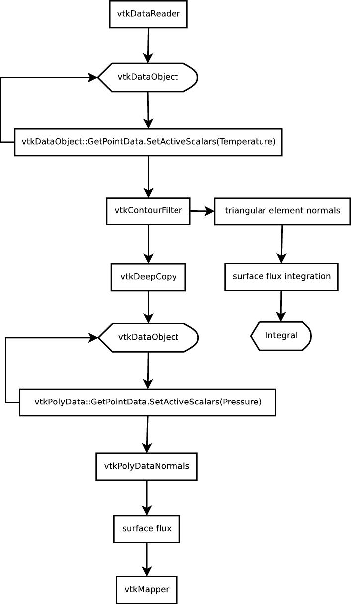
Figure 1: Data flow for flux visualisation and integration.

3.1 Isosurface probe

To compute these examples we created a new MayaVi filter declared as a class:

class IsoSurfaceProbe (Base.Objects.Filter):
  ...

The data flow of this filter is illustrated in Figure 1. The filter first calculates an isosurface (using the VTK class vtkContourFilter) for the active scalar field (which can be selected using the MayaVi graphical user interface (GUI)). Regardless of the element type in the input data (meaning that this filter can be applied to model output from any of the models described in the introduction), the isosurface itself is comprised of piecewise-linear triangular elements; any non-triangular polygons are triangulated (and quadratic triangular elements are split into four linear triangle elements). The normals obtained are self-consistently oriented on each connected surface. Scalars and vectors from the input data are automatically interpolated using the finite element basis functions onto the vertices of the isosurface. The contour filter is set up simply by calling the constructor

self.cont_fil = vtk.vtkContourFilter ()

The input to the contour filter object is set in the SetInput method:

self.cont_fil.SetInput (source.GetOutput ())

For reasons that will become clear in the next section, we make a deep copy of the output to self.iso

self.iso = vtk.vtkPolyData ()
...
self.iso.DeepCopy (self.cont_fil.GetOutput ())

and set the copy as the output to the filter

def GetOutput (self):
  return self.iso

so that the data can be visualised.

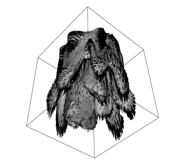
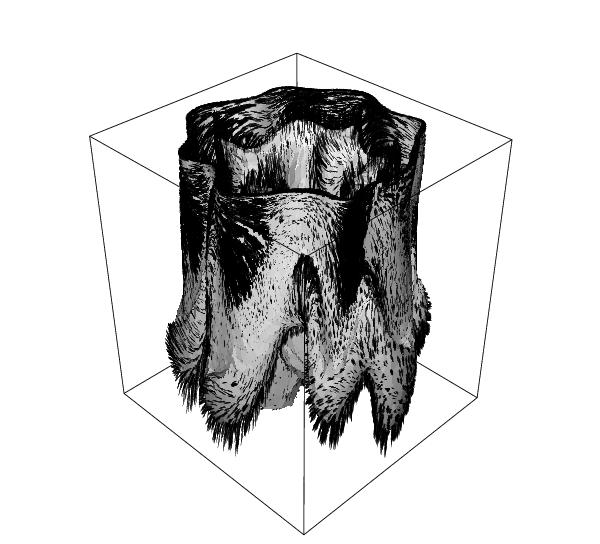
Figure 2: Plots showing the temperature $T-T_{0}=0.02869K$ isosurface, together with superimposed velocity vectors projected onto the surface, viewed from above and below. The geostrophic rim currents are most clearly visible in the view from above, whereas the view from below shows the velocity of the rapidly descending plumes.

The output from the filter can be displayed using the standard MayaVi modules without any further coding. In Figure 2 the surface map module is used to display an isopycnal surface, with velocity vectors superimposed. This allows the dynamics of this particular isopycnal surface to be studied. One can see that the velocity vectors are pointing around the rim of the water column at the ocean surface in accordance with geostrophic balance, but also strong downward flow at the head of the descending plumes. See (Jones and Marshall, 1993) for a description of the dynamical processes.

3.2 Additional fields

In many cases it is desirable to add additional diagnostic fields to the output of the contour filter. However, if the active scalar of the output from the contour filter is modified, this will actually change the active scalar of the original data object passed into the contour filter. For this reason it is necessary to make a copy of the result of the contour filter (See Figure 1). With this copy, new data fields can be added and the active scalar (or vectors) can be changed. This allows one to visualise arbitrary field data on the isosurface.

In our filter, the volume flux ${\boldsymbol{u}}\cdot{\boldsymbol{n}}$ is calculated, where ${\boldsymbol{u}}$ is the velocity calculated at the isosurface vertices and ${\boldsymbol{n}}$ is the normal vertices calculated using the VTK class vtkPolyDataNormals class. The normals are calculated as points data on the triangle vertices,

normal_calculator = vtk.vtkPolyDataNormals()
normal_calculator.SetInput(self.GetOutput())
normal_calculator.Update()
normals = normal_calculator.GetOutput().GetPointData().GetNormals()

and then the volume flux is computed and added to the data set.

volume_flux_array = vtk.vtkDoubleArray()
volume_flux_array.SetNumberOfTuples(n_points)
volume_flux_array.SetName(’VolumeFlux’)
vecs = self.GetOutput().GetPointData().GetVectors()
for i in range(n_points):
  (u,v,w) = vecs.GetTuple3(i)
  (n1,n2,n3) = normals.GetTuple3(i)
  volume_flux = u*n1 + v*n2 + w*n3
  volume_flux_array.SetTuple1(i, volume_flux)
self.iso.GetPointData().AddArray(volume_flux_array)
self.iso.GetPointData().SetActiveAttribute(’VolumeFlux’,0)

The volume flux is shown in Figure 3, visualised using the Mayavi SurfaceMap module together with a zero contour produced by the IsoSurface module. This field shows where the isopycnal surface is expanding and where it is contracting, i.e. it illustrates how the isopycnal surface is being advected by the flow. This can be used for diagnosing mixing in the flow as it shows how small scales are formed in the temperature field. In Figure 4 a gradient map for nonhydrostatic pressure is projected onto the same isopycnal to illustrate this. This plot allows one to study the relative size of nonhydrostatic pressure in different parts of the convective structure. The plot shows that nonhydrostatic pressure is greatest near to the plumes at the centre of the convection cell. Pressure is a global quantity arising from the pressure Poisson equation so this should not form a complete guide to nonhydrostatic effects, however it does reveal that there is significant nonhydrostatic dynamics in the flow.

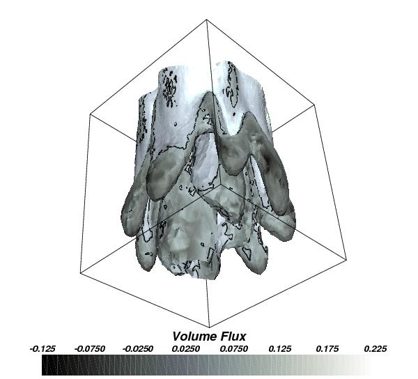
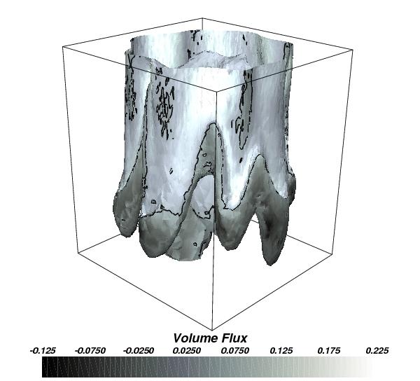
Figure 3: Plots showing the temperature $T-T_{0}=0.02869K$ isosurface with a gradient map representing volume flux, viewed from above and below. Black lines are used to mark the volume flux zero contour on the surface. Negative volume flux indicates the isosurface is locally expanding and positive volume flux indicates the isosurface is locally contracting (the overall sign depends on how VTK orients the surface; this is done self-consistently on each connected surface). The plots show that the isosurface is expanding at the bottom and shrinking at the top i.e. it is being stretched out by the flow. This stretching occurs to satisfy incompressibility of the flow.

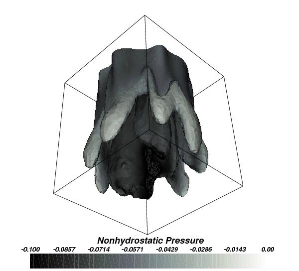
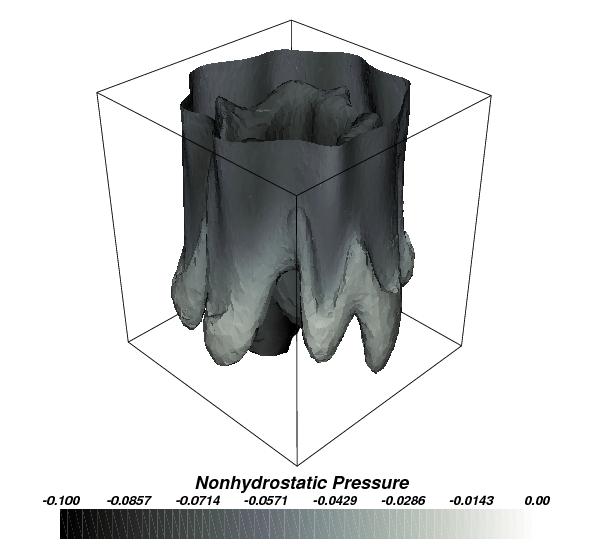
Figure 4: Plots showing the temperature $T-T_{0}=0.02869K$ isosurface with a gradient map representing nonhydrostatic pressure, viewed from above and below. The nonhydrostatic pressure has the largest magnitude around the descending plumes inside the convection cell.

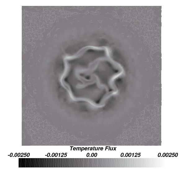
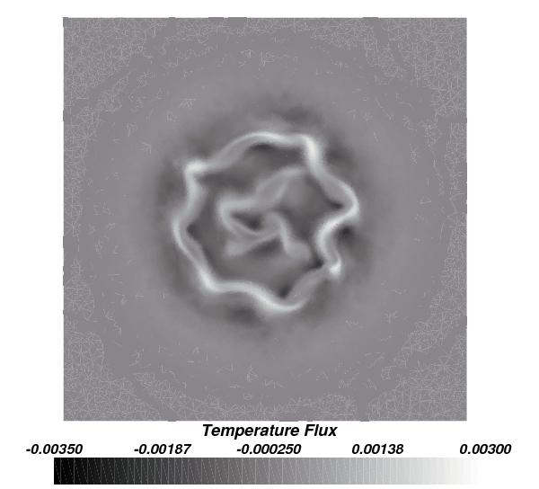
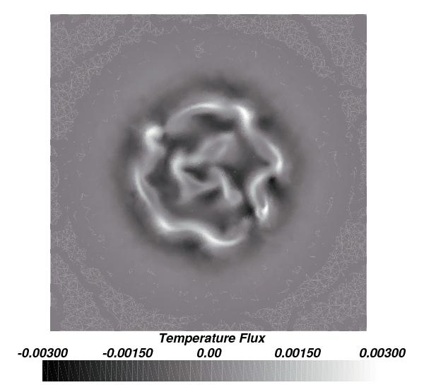
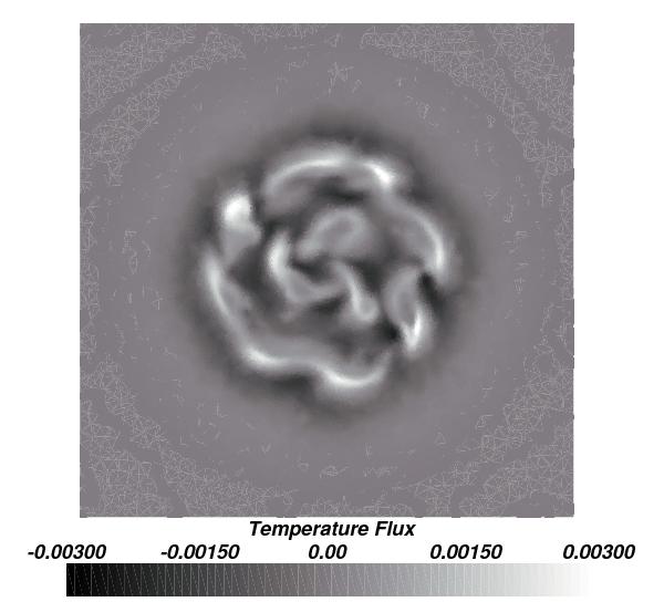
Figure 5: Plots showing temperature flux through horizontal surfaces of different levels, defined as isosurfaces of the initial condition for temperature. The levels are: $T-T_{0}=0.07$ (top-left), $T-T_{0}=0.065$ (top-right), $T-T_{0}=0.06$ (bottom-left) and $T-T_{0}=0.055$ (bottom-right). These plots illustrate how temperature is being transported by the convection cell.

From this point many other diagnostic quantities can readily be calculated. For example, the temperature advective flux, $T{\boldsymbol{u}}\cdot{\boldsymbol{n}}$ where $T$ is temperature, through a number of horizontal slices is shown in Figure 5. It shows downward transport of temperature inside the plume structures and a weak upwelling in-between.

3.3 Flux calculation

Mayavi filters and modules can also be used to compute integrals over the surface. This is done by looping over the triangular faces in the surface and calculating the contribution from each face using the piecewise-linear representation.

For a vector field ${\boldsymbol{F}}$, the flux through an isosurface $S$ is defined as

$$\int_{S}{\boldsymbol{F}}\cdot{\boldsymbol{n}}dS,$$

where $S$ is the isosurface, and ${\boldsymbol{n}}$ is the normal to that surface. On a piecewise-linear triangular mesh, this is expressed discretely as:

$$\sum_{e=1}^{E}A_{e}{\boldsymbol{F}}_{e}\cdot{\boldsymbol{n}}_{e},$$ (1)

where $E$ is the total number of triangular elements defining the surface, ${\boldsymbol{F}}_{e}$ is the mean value of ${\boldsymbol{F}}$ on triangle $e$, $A_{e}$ is the area of triangle $e$ and ${\boldsymbol{n}}_{e}$ is the normal to triangle $e$.

The flux calculation function in the class makes repeated use of VTK data retrieval routines. First it gets vtkDataArray variables which point to the active vectors and scalars.

def calc_flux (self, event=None):
  ...
  point_to_cell = vtk.vtkPointDataToCellData ()
  point_to_cell.SetInput (self.GetOutput ())
  point_to_cell.Update ()
  vecs = point_to_cell.GetOutput ().GetCellData ().GetVectors ()
  fluxf = self.GetOutput().GetCellData().GetScalars()

Next, it loops over the cells (elements) in the isosurface, computes the cell area and normals,

  for cell_no in range(n_cells):
    Cell = self.GetOutput().GetCell(cell_no)
    ...
    Cell_points = Cell.GetPoints ()
    Area = Cell.TriangleArea(Cell_points.GetPoint(0), \
                             Cell_points.GetPoint(1), \
                             Cell_points.GetPoint(2))
    n = [0.0,0.0,0.0]
    Cell.ComputeNormal(Cell_points.GetPoint(0), \
                       Cell_points.GetPoint(1), \
                       Cell_points.GetPoint(2), n)

then it gets the values of the active vectors and scalars in each cell and computes the volume and scalar fluxes.

    (u,v,w) = vecs.GetTuple3(cell_no)
    f = Area*(u*n[0] + v*n[1] + w*n[2])
    Integral_volume_flux = Integral_volume_flux + f
    ...
    s = fluxf.GetTuple1(cell_no)
    scalar_advected_flux = scalar_advected_flux + s*f

As a test example, we integrated the flux of velocity (volume flux) over the temperature isosurface $T-T_{0}=0.02171Km^{-2}s^{-1}$, obtaining an integral $I=-3.60\times 10^{5}s^{-1}$. For a divergence-free vector field we should obtain zero; this computed value is small compared to the total area ($3.4\times 10^{8}m^{2}$) of this surface so the numerical errors from the fluids code and from the integration are small. We also computed advective integrated temperature fluxes (flux of $(T-T_{0}){\boldsymbol{u}}$) over the levels displayed in Figure 5 which are displayed in the following table:

Initial value of $T-T_{0}$	Temperature flux through surface
$0.055K$	$-7.14\times 10^{4}Ks^{-1}$
$0.06K$	$-7.24\times 10^{4}Ks^{-1}$
$0.065K$	$-6.44\times 10^{4}Ks^{-1}$
$0.07K$	$-3.62\times 10^{4}Ks^{-1}$

As Mayavi/VTK uses the finite element representation of the solutions fields (in this paper we restricted ourselves to piecewise-linear tetrahedral elements), the construction of the isosurface and the evaluation of flux integrals are exact for the given finite element representation. This means that the accuracy of the flux integrals are entirely determined by how well the solution fields are represented on the mesh. To illustrate this, we took a series of isotropic, homogeneous, unstructured grids in a cube with dimensions $1\times 1\times 1$, and evaluated the field

$$T=\sqrt{(X-0.5)^{2}+(Y-0.5)^{2}+(Z-0.5)^{2}}$$

at the grid points. We computed the $T=0.5$ isosurface and calculated the flux of the vector field

$${\boldsymbol{F}}=(X,Y,Z)$$

through the isosurface, which has the exact integral

$$\int_{T=0.5}{\boldsymbol{F}}\cdot{\boldsymbol{n}}\operatorname{d}{S}=\pi.$$

Plots of example isosurfaces are given in Figure 6. A plot of the error in the computed flux is given in Figure 7. We note that whilst these meshes are isotropic and homogeneous, a more efficient way to ensure that the fields are well-represented on the mesh is to use anistropic dynamic adaptivity during the calculation of the flow solution. In this case the accuracy of the flux integrals (as well as the solution itself) will be determined by the metric used to construct the mesh.

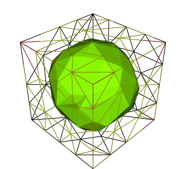
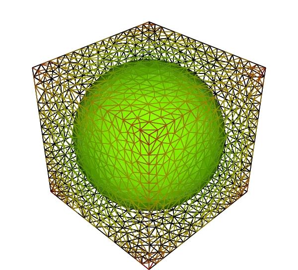
Figure 6: Plots showing example isosurfaces used to check the convergence of flux integrals, with average cell volume 0.01 (top plot) and average 0.0001 (top plot).

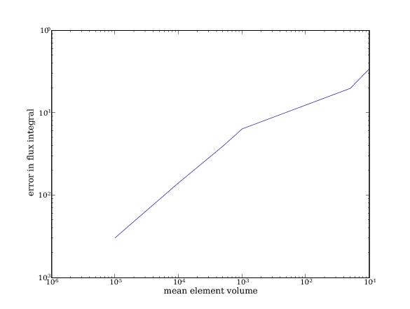
Figure 7: Plot showing error of computed flux against average tetrahedral volume for a flux computation on a structured mesh.

4 Summary and Outlook

In this paper we describe a strategy for obtaining diagnostic information from unstructured adaptive ocean model output by adding modules and filters to the open source visualisation package MayaVi using the VTK graphics library. We explained this strategy with the example of an isosurface probe filter which interpolates flow data onto an isosurface of a chosen field, and constructs flux quantities across the isosurface which may then be visualised and integrated. We illustrated all of this using unstructured flow data from a deep convection experiment using ICOM.

The strength of the finite element method is that it provides a representation of the solution fields everywhere in space via the finite element basis functions, i.e. not just at the nodal points where the data is stored. This means that structures such as isosurfaces are well-defined, as are integrals. Additionally, when the solution has been evolved using an adaptive unstructured mesh constructed from an error metric (Pain et al., 2001) the error in the integral is bounded by construction.

Python and VTK provides a convenient way to construct new fields and to calculate integral quantities, and the use of pipelines maximises the interactivity of any modules and filters added to MayaVi. This interactivity is an important part of scientific analysis and exploration of data. Modules and filters are written using the Python scripting language which means that it is relatively quick to develop new analysis tools as the need arises without a deep understanding of the software. The open source environment provides the opportunity for rapid scientific advance and collaboration.

5 Acknowledgements

This paper began after conversations about diagnostic calculations on unstructured grids with Katya Popova. The authors would like to acknowledge all the ICOM developers for their collaborative support. The deep convection simulation data was provided by Lucy Bricheno. This work was partially supported by the NERC RAPID Climate Change grant NER/T/S/2002/00459 and the NERC Consortium grant NE/C52101X/1. Thanks to Prabhu Ramachandran for developing and maintaining the MayaVi project and for responding so helpfully to our questions and queries.

References

- Aikman et al. (2006) Aikman, F., Beegle-Krause, C., Hankin, S., Gross, T., October 2006. Report on the workshop: Community standards for unstructured grids. Tech. rep., Boulder, Colorado, US.
- Jones and Marshall (1993) Jones, H., Marshall, J., 1993. Convection with rotation in a neutral ocean: A study of. open-ocean deep convection. J. Phys. Oceanography 23, 1009–1039.
- Oliphant (2007) Oliphant, T., May 2007. Python for scientific computing. Computing in Science & Engineering 9 (3).
- Pain et al. (2005) Pain, C., Piggott, M., Goddard, A., Fang, F., Gorman, G., Marshall, D., Eaton, M., Power, P., de Oliveira, C., 2005. Three-dimensional unstructured mesh ocean modelling. Ocean Modelling 10, 5–33.
- Pain et al. (2001) Pain, C. C., Umpleby, A. P., de Oliveira, C. R. E., Goddard, A. J. H., 2001. Tetrahedral mesh optimisation and adaptivity for steady state and transient finite element calculations. Comput. Methods Appl. Mech. Eng., 3771–3796.
- Ramachandran (2001) Ramachandran, P., 2001. Mayavi: A free tool for CFD data visualization. In: 4th Annual CFD Symposium. Aeronautical Society of India.