Abstract

The energy in a square membrane $\Omega$ subject to constant viscous damping on a subset $\omega\subset\Omega$ decays exponentially in time as soon as $\omega$ satisfies a geometrical condition known as the “Bardos-Lebeau-Rauch” condition. The rate $\tau(\omega)$ of this decay satisfies $\tau(\omega)=2\min(-\mu(\omega),g(\omega))$ (see Lebeau [9]). Here $\mu(\omega)$ denotes the spectral abscissa of the damped wave equation operator and $g(\omega)$ is a number called the geometrical quantity of $\omega$ and defined as follows. A ray in $\Omega$ is the trajectory generated by the free motion of a mass-point in $\Omega$ subject to elastic reflections on the boundary. These reflections obey the law of geometrical optics. The geometrical quantity $g(\omega)$ is then defined as the upper limit (large time asymptotics) of the average trajectory length. We give here an algorithm to compute explicitly $g(\omega)$ when $\omega$ is a finite union of squares.

MSC Numbers: 35L05, 93D15 Key words: Damped wave equation, mathematical billards

Let $\Omega=[0,1]^{2}$ be the unit square of $\mathbb{R}^{2}$ and let $\omega\subset\Omega$ be a subdomain of $\Omega$. We are interested here in the problem of uniform stabilization of solutions of the following equation

$$\begin{cases}u_{tt}(x,t)-\Delta u(x,t)+2\chi_{\omega}(x)u_{t}(x,t)=0,\;x\in\stackrel{{\scriptstyle\circ}}{{\Omega}},\,t>0,\\ u(x,t)=0,\;x\in\partial\Omega,\,t>0\\ u(.,0)=u_{0}\in H^{1}_{0}(\Omega),\\ u_{t}(.,0)=u_{1}\in L^{2}(\Omega),\end{cases}$$ (0.1)

where $\chi_{\omega}$ is the characteristical function of the subset $\omega$. This equation has its origin in a physical problem. Consider a square membrane $\Omega$. We study here the behaviour of a wave in $\Omega$. Let $u(x,t)$ be the vertical position of $x\in\Omega$ at time $t>0$. We assume that we apply on $\omega$ a force proportional to the speed of the membrane at $x$. Then, $u$ satisfies equation (0.1). To get more information on this subject, one can refer to [7], [10], [2]. With regard to the one-dimensional case, the reader can consult [6] and [3].

We do not deal here with the existence of solutions. We assume that there exists a solution $u$. Let us define the energy of $u$ at time $t$ by

$$E(t)=\int_{\Omega}{|\nabla u|}^{2}+u_{t}^{2}dx.$$

It is well known that, for any $t\geq 0$,

$$E(t)\leq CE(0)\hbox{e}^{-2\tau t},$$ (0.2)

where $C,\tau\geq 0$. As proven by E. Zuazua [13], this result remains true in the semilinear case when the dissipation is in a neighborhood of a subset of the boundary satisfying the multiplier condition. Let us now define

Definition 0.1

The exponential rate of decay $\tau(\omega)$ is defined by

$$\tau(\omega)=sup\{\tau\geq 0\hbox{ s.t. }\exists C>0\hbox{ for which }(\ref{a_1})\hbox{ holds }\}.$$

Many articles have been devoted to finding bounds for $\tau(\omega)$. The reader can consult [1], [9] and [11]. In the case of a non-constant damping, the reader may see [4]. G. Lebeau proved in [9] that

$$\tau(\omega)=2\min(-\mu(\omega),g(\omega)).$$

Here $\mu(\omega)$ denotes the spectral abscissa of the damped wave equation operator and $g(\omega)$ is a number called the geometrical quantity of $\omega$ and defined as follows. A ray in $\Omega$ is the trajectory generated by the free motion of a mass-point in $\Omega$ subject to elastic reflections in the boundary. These reflections obey the law of geometrical optics: the angle of incidence equals the angle of reflection. If a ray meets a corner of $\Omega$, the reflection will be the limit of the reflection of the rays which go to this corner. It is easy to verify that the ray runs along the same trajectory before and after the reflection but in an opposite direction.

Let $\gamma:\mathbb{R}^{+}\rightarrow\Omega$ be the parametrization of the ray by arclength. Let

$$\mathcal{C}=\big{\{}\hbox{ rays in }\Omega\big{\}}.$$

Furthermore, let $\rho_{0}=(X_{0},\alpha)$, where $X_{0}\in\Omega$ and $\alpha\in[0,2\pi[$. Consider the ray $\gamma_{\rho_{0}}$ which starts at $X_{0}$ in the direction of the vector $(\cos(\alpha),\sin(\alpha))$. Each ray of $\mathcal{C}$ can be defined in this way. More precisely, if $\Gamma=\Omega\times[0,2\pi[$ then

$$\mathcal{C}=\{\gamma_{\rho_{0}}\hbox{ s.t. }\rho_{0}\in\Gamma\}.$$

In the whole paper $\gamma\in\mathcal{C}$ will be noted $\gamma=[X_{0},\alpha]$. If $\gamma\in\mathcal{C}$ and if $t>0$ is a positive real number, we write:

$$\gamma_{t}=\gamma_{/[0,t]}.$$

Let

$$\mathcal{C}^{\prime}=\bigcup_{t>0}\big{\{}\gamma_{t}\big{|}\gamma\in\mathcal{C}\big{\}}$$

be the set of paths of finite length not necessarily closed. For $\gamma_{t}\in\mathcal{C}^{\prime}$ of length $t>0$, we define:

$$m(\gamma_{t})=\frac{1}{t}\int_{0}^{t}\mathcal{X}_{\omega}(\gamma_{t}(s))ds.$$

The definition of $m$ can be extended to $\mathcal{C}$. Indeed, if $\gamma\in\mathcal{C}$, set

$$m(\gamma)=\limsup_{t\to+\infty}m(\gamma_{t}).$$

It is proven in Section 1.2 that

$$m(\gamma)=\lim_{t\to+\infty}m(\gamma_{t}).$$ (0.3)

For a ray $\gamma$ belonging to $\mathcal{C}$, $m(\gamma)$ represents the average time that $\gamma$ spends in $\Omega$.

Definition 0.2

The geometrical quantity $g(\omega)$ is defined by

$$g(\omega)=\limsup_{t\to+\infty}\inf_{\gamma\in\mathcal{C}}m(\gamma_{t}).$$

We are interested here in a precise study of the geometrical quantity $g$. The first part of this paper is devoted to studying the rays. We recall some well known properties of rays. In the second part, another expression for $g$ is given. Namely, we prove that if $\omega\subset\Omega$ whose boundary is a finite union of $C^{1}$-curves, then

$$g(\omega)=\inf_{\gamma\in\mathcal{C}}\limsup_{t\to+\infty}m(\gamma_{t})=\inf_{\gamma\in\mathcal{C}}m(\gamma).$$

It is easier to work with this second definition of $g(\omega)$. An important application of this theorem is given in the third part: we obtain an algorithm which gives an exact computation of $g(\omega)$ when $\omega$ is a finite union of squares. This work has many interests. At first, Theorem 2.1 gives another definition for $g(\omega)$, much more easy to manipulate than the original one. Secondly, maximizing the exponential rate of decay is interesting from the point of view of physics. For these questions, knowing exactly $g(\omega)$ is important. We give some exact computations of $g(\omega)$ with the help of our algorithm at the end of the paper. An interesting question is then: how can we choose the subset $\omega$ such that $g(\omega)$ is maximum? At the moment, this problem is still open. The following inequality is always true $g(\omega)\leq|\omega|$ (see Section 2) where $|\omega|$ is the area of $\omega$. Let us set for $\alpha\in[0,1]$

$$\mathcal{S}(\alpha)=\sup_{|\omega|=\alpha}g(\omega).$$

Some questions then arise naturally

- What is the value of $\mathcal{S}(\alpha)$? In particular, is it true that $\mathcal{S}(\alpha)=\alpha$?

- Can we find a subset $\omega$ for which $g(\omega)=|\omega|$?

- Can we find an optimal $\omega$ (i.e.  an $\omega$ that maximizes $g$) among the domains that satisfy the multiplier condition?

If $|\omega|=0$ or $|\omega|=1$, the answers are obvious. However, if $|\omega|\in]0,1[$, these questions seem to be much more difficult and are still open.

1 Basic properties of rays

1.1 Different representations of rays

In this section, we regard billards in $\Omega$ from different point of views (see for example [12]). Instead of reflecting the trajectory with respect to a side of $\Omega$, one can reflect $\Omega$ with respect to this side. We then obtain a square grid and the initial trajectory is straightened to a line. This gives a correspondance between billard trajectories in $\Omega$ and straight lines in the plane equipped with a square grid. Two lines in the plane correspond to the same billard trajectory if they differ by a translation through a vector of the lattice $2\mathbb{Z}+2\mathbb{Z}$. The factor $2$ in $2\mathbb{Z}+2\mathbb{Z}$ is important. Indeed, two adjacent squares have an opposite orientation in the sense that they are symmetric with respect to their common side.

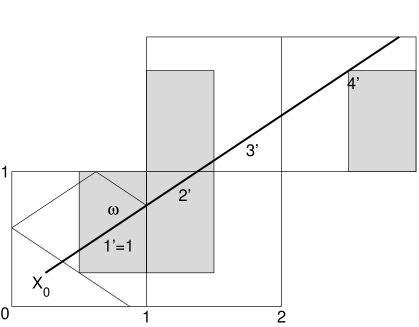
Figure 1: Point of view of infinite plane

Now, consider $T={[0,2]}^{2}$ and identify its opposite sides. A trajectory then becomes a geodesic line in the flat torus.

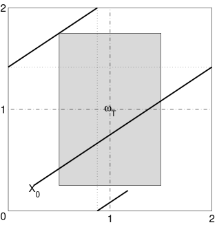
Figure 2: Point of view of flat torus

Finally, trajectories in $\Omega$ can be seen in three different ways

- the definition which consists in reflecting trajectories in sides of $\Omega$

- the point of view of straight lines in $\mathbb{R}^{2}$

- the point of view of geodesic lines in a flat torus $T$.

Note that the set $\omega$ must be reflected in the same way as we did for $\Omega$. This means that the sets $\omega$ contained in two adjacent squares must be symmetric with respect to their common side (see Figures 1 and 2).

Let $t>0$ and $\gamma\in\mathcal{C}$. The value

$$\frac{1}{t}\int_{0}^{t}\mathcal{X}_{\omega}(\gamma_{t}(s))ds$$

does not depend on the point of view we adopt.

1.2 Open and closed rays

A ray is said to be closed if it is periodic in the flat torus. It is said to be open if it is not closed. We have the following characterization. The ray $[X_{0}=(x_{0},y_{0}),\alpha]$ is open if and only if $\cos\alpha$ and $\sin\alpha$ are independent over $\mathbb{Z}$, i.e. if and only if $\tan\alpha\in\mathbb{R}-\mathbb{Q}$. Indeed, for example using the point of view of a flat torus, the trajectory is periodic if and only if there exist $0\leq t_{1}<t_{2}$ and $n,m\in\mathbb{N}$ such that

$$\left\{\begin{array}[]{ll}x_{0}+t_{1}\cos\alpha=x_{0}+t_{2}\cos\alpha+2n\\ y_{0}+t_{1}\sin\alpha=y_{0}+t_{2}\sin\alpha+2m\end{array}\right..$$

Hence $2m(t_{1}-t_{2})\cos\alpha-2n(t_{1}-t_{2})\sin\alpha=0$. Let us now consider open rays. They have the following properties (see for example [5] p. 172).

Proposition 1.1

Let $\gamma=[X_{0},\alpha]$ be an open ray. Then, $\{\gamma_{t},\,t\geq 0\}$ is dense in the torus $T$ and then in $\Omega$. In addition, if $\omega$ is quarrable (i.e. $\chi_{\omega}$ Riemann-integrable on $\Omega$) then $m(\gamma_{t})\xrightarrow[t\to+\infty]{}|\omega|$. More precisely, let $\alpha$ be such that $\tan\alpha\in\mathbb{R}-\mathbb{Q}$ then

$$\forall\epsilon>0,\,\exists t_{0}\,|\,t\geq t_{0},\forall X_{0}\in\Omega\;:\;\text{if}\;\gamma_{\rho_{0}}=[X_{0},\alpha]\;\text{then}\;\left|m(\gamma_{t})-|\omega|\right|<\epsilon.$$

In other words, $t_{0}$ is independent of $X_{0}$.

Here, $|\omega|$ stands for the area of $\omega$. Consider now closed rays. They satisfy the following properties:

Proposition 1.2

Let $\gamma=[X_{0},\alpha]$ be a closed ray. Then, there exist $p,q\in\mathbb{Z}$ relatively prime such that:

$$\cos\alpha=\frac{p}{\sqrt{p^{2}+q^{2}}}\quad\text{and}\quad\sin\alpha=\frac{q}{\sqrt{p^{2}+q^{2}}}.$$

The period $L$ of the trajectory is $L=2\sqrt{p^{2}+q^{2}}$. We have

$$m(\gamma_{t})\xrightarrow[t\to+\infty]{}\frac{1}{L}\int_{0}^{L}\chi_{\omega}(\gamma(s))ds.$$

Remark 1.1

The assertion (0.3) follows immediately from Propositions 1.1 and 1.2. Moreover, let $\gamma\in\mathcal{C}$. If $\gamma$ is open, we have $m(\gamma)=|\omega|$ and if $\gamma$ is periodic of period $L$, we have $m(\gamma)=\frac{1}{L}\int_{0}^{L}\chi_{\omega}(\gamma(s))ds$.

As one can check, an immediate consequence of Proposition 1.2 is the following result

Proposition 1.3

Let $\omega\subset\Omega$ be Riemann-integrable, then

$$g(\omega)\leq|\omega|.$$

Closed rays can easily be described. Let us adopt the point of view of a flat torus. Let us consider a ray $\gamma=[X_{0},\alpha]$ with $X_{0}\in T$ and $\cos\alpha=p/\sqrt{p^{2}+q^{2}},\,\sin\alpha=q/\sqrt{p^{2}+q^{2}}$, $p$ and $q$ relatively prime. We assume that $p\geq 0$ and $q\geq 0$ (i.e $\alpha\in[0,\pi/2]$). From remark 3.1 below, the study can be restricted to such rays.

Theorem 1.1

The ray $\gamma$ is an union of $p+q$ parallel segments directed by $\vec{u}=\cos\alpha\,\vec{i}+\sin\alpha\,\vec{j}$. Among these segments, $p$ of them start at $A_{k}$, $1\leq k\leq p$, and the $q$ others start at $B_{k}$, $1\leq k\leq q$ with

$$A_{k}\,\left(0,\big{(}y_{0}+q/p(2k-x_{0})-2E(\frac{1}{2}(y_{0}+q/p(2k-x_{0}))\big{)}\right)$$

and

$$B_{k}\,\left(\big{(}x_{0}+p/q(2k-y_{0})-2E(\frac{1}{2}(x_{0}+p/q(2k-y_{0}))\big{)},0\right)).$$

In addition, the distance between two neighbouring segments is constant and equal to $\delta=4/L$, where $L=2\sqrt{p^{2}+q^{2}}$ is the period.

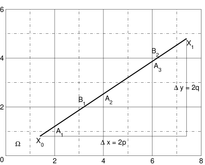
Figure 3: Closed ray for $p=3$ and $q=2$ in the infinite plane

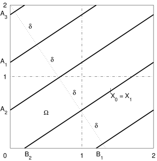
Figure 4: Closed ray $p=3$ and $q=2$ in the flat torus

Proof : In the infinite plane $\mathbb{R}^{2}$, the ray is defined by $x(t)=x_{0}+2tp/L$ and $y(t)=y_{0}+2tq/L$, where $L=2\sqrt{p^{2}+q^{2}}$ is the period. Let us restrict the study to the segment $[X_{0}X_{1}]$ of length $L$. In $]X_{0}X_{1}[$, the ray intersects $p$ vertical straight lines defined by the equations $x=2k,\,k=1,\cdots,p$ and $q$ horizontal straight lines defined by the equation $y=2k,\,k=1,\cdots,q$. This gives $p+q$ segments starting at points with coordinates

$$\big{(}0,y_{0}+q/p(2k-x_{0})\big{)}$$

and

$$\big{(}x_{0}+p/q(2k-y_{0}),0\big{)}.$$

Coming back to the point of view of the torus, this gives $p+q$ segments starting at $A_{k}$ and $B_{k}$.
Since $p$ and $q$ are relatively prime, it is well known that $\{kq\,[p],\,1\leq k\leq p\}=\{0,1,\dots,p-1\}$. Hence, if $A_{k_{1}}$ and $A_{k_{2}}$ are two neighbouring points, $A_{k_{1}}A_{k_{2}}=2/p$. As a consequence, the distance between the straight lines $(A_{k_{1}},\vec{u})$ and $(A_{k_{2}},\vec{u})$ is

$$\delta=\left|\overrightarrow{A_{k_{1}}A_{k_{2}}}.\vec{u}^{\bot}\right|=\frac{2}{p}\,\vec{j}.\frac{-q\vec{i}+p\vec{j}}{\sqrt{p^{2}+q^{2}}}=\frac{4}{L}.$$

In the same way, if $B_{k_{1}}$ and $B_{k_{2}}$ are two neighbouring points $B_{k_{1}}B_{k_{2}}=2/q$, the distance between $(B_{k_{1}},\vec{u})$ and $(B_{k_{2}},\vec{u})$ is

$$\delta=\left|\overrightarrow{B_{k_{1}}B_{k_{2}}}.\vec{u}^{\bot}\right|=\frac{2}{q}\,\vec{i}.\frac{q\vec{i}-p\vec{j}}{\sqrt{p^{2}+q^{2}}}=\frac{4}{L}.$$

Let $k_{1}$, $k_{2}$ be such that

$$dist(A_{k_{1}},0)=\min_{k}dist(A_{k},0)\hbox{ and }dist(B_{k_{2}},0)=\min_{k}dist(B_{k},0).$$

It remains to prove that the distance between the two segments starting at $A_{k_{1}}$ and $B_{k_{2}}$ is $\delta=4/L$. Since the distance between two points $A_{k}$ is $2/p$, there exists $n\in\mathbb{N}$ such that the ordinate $y^{*}$ of $A_{k_{1}}$ satisfies

$$\begin{split}2n&\leq y_{0}+q/p(2k_{1}-x_{0})-2E(\frac{1}{2}(y_{0}+q/p(2k_{1}-x_{0}))<2n+2/p\\ &\;\Longrightarrow\;y^{*}=y_{0}+q/p(2k_{1}-x_{0})-2E(\frac{1}{2}(y_{0}+q/p(2k_{1}-x_{0}))-2n<2/p.\end{split}$$

In the same way, there exists $m\in\mathbb{N}$ such that the abscissa $x^{*}$ of $B_{k_{2}}$ satisfies

$$\begin{split}2m&\leq x_{0}+p/q(2k_{2}-y_{0})-2E(\frac{1}{2}(x_{0}+p/q(2k_{2}-y_{0}))<2m+2/q\\ &\;\Longrightarrow\;x^{*}=x_{0}+p/q(2k_{2}-y_{0})-2E(\frac{1}{2}(x_{0}+p/q(2k_{2}-y_{0}))-2m<2/q.\end{split}$$

The distance $\delta$ between the two segments verifies:

$$\delta=\left|\overrightarrow{A_{k_{1}}B_{k_{2}}}.\vec{u}^{\bot}\right|=\frac{|qx^{*}+py^{*}|}{\sqrt{p^{2}+q^{2}}}.$$

An easy computation shows that $|qx^{*}+py^{*}|$ is an even integer number. Consequently, $\delta$ can be written as $4k/L$, where $k$ is an integer. Since $0\leq x^{*}<2/q$ and $0\leq y^{*}<2/p$, we get $\delta<8/L$, and hence, $\delta=4/L$. $\square$

Remark 1.2

If a quarrable domain $\omega$ is such that $g(\omega)=|\omega|$ then for all $\alpha\in[0,\pi/2]$ and for almost all $X_{0}\in T$, $m(\gamma)=|\omega|$, where $\gamma=[X_{0},\alpha]$.

Indeed, consider an open ray $\gamma$. Then $m(\gamma)=|\omega|$. Let $X_{0}\in\Omega$. Assume that a ray $\gamma$ starting at $X_{0}$ is closed of length $L$. Let $M$ and $N$ be two points of $\gamma$ such that $\overrightarrow{MN}$ is orthogonal to $\vec{u}$ and $MN=\delta$. Let also $P(s)=sM+(1-s)N$ and $\gamma^{s}=[P(s),\alpha]$, then

$$g(\omega)\leq\inf_{s\in[0,1]}m(\gamma_{L}^{s})\leq\int_{0}^{1}m(\gamma_{L}^{s})ds\leq|\omega|.$$

If $g(\omega)=|\omega|$, then $m(\gamma_{L}^{s})=|\omega|$ almost everywhere. If $\partial\omega$ is a finite union of curves of class $C^{1}$, then the number of discontinuity points of $m(\gamma_{L}^{s})$ is finite. It is null if $\partial\omega$ does not possess any segments. The remark above immediately follows.

2 An equivalent definition for $g$

2.1 The geometrical quantity $g^{\prime}$

We define, for any set $\omega$:

Definition 2.1

The geometrical quantity $g^{\prime}(\omega)$ is defined by

$$g^{\prime}(\omega)=\inf_{\gamma\in\mathcal{C}}m(\gamma).$$

As easily seen, $g^{\prime}$ is easier to study than $g$. As shown in Section 3, $g^{\prime}(\omega)$ can be computed explicitly for a certain class of domains $\omega$. Together with Theorem 2.1, this gives an algorithm for computing $g(\omega)$.

Theorem 2.1

Let $\omega$ be a closed set whose boundary is a finite union of curves of class $C^{1}$. Then

$$g(\omega)=g^{\prime}(\omega).$$

As a first remark, the same argument as in the proof of Proposition 1.3 shows that

$$0\leq g^{\prime}(\omega)\leq|\omega|.$$ (2.1)

The proof of Theorem 2.1 is given in the appendix. It is easy to see that $g(\omega)\leq g^{\prime}(\omega)$. Inequality $g^{\prime}(\omega)\leq g(\omega)$ is much more difficult to obtain. To prove Theorem 2.1, we consider a sequence of rays $\gamma^{n}=[x_{n},\theta_{n}]$ and a sequence of real numbers $t_{n}\to+\infty$ for which $m(\gamma^{n}_{t_{n}})\to g(\omega)$. After choosing a subsequence, there exists $(x,\theta)\in\Omega\times[0,2\pi[$ such that $\lim_{n}x_{n}=x$ and $\lim_{n}\theta_{n}=\theta$. We will now show that $\lim_{n}m(\gamma^{n}_{t_{n}})-m([x,\theta]_{t_{n}})=0$. The conclusion then follows. The difficulty in this proof is that the function $(x,\theta)\to m([x,\theta]_{t})$ is not continuous. A direct consequence of Theorem 2.1 is that it suffices to consider closed rays in the explicit computation of $g(\omega)$. Namely, let $\mathcal{C}_{c}$ be the set of closed rays, then we have:

$$g(\omega)=\inf_{\gamma\in\mathcal{C}_{c}}m(\gamma).$$ (2.2)

3 Explicit computation of $g$

We prove in this section that for a particular class of domains $\omega$, the properties of the geometrical quantity $g$ we obtain above allow to compute explicitly $g(\omega)$. Let $N\in\mathbb{N}^{*}$, and let $\omega\subset\Omega$ be a finite union of squares $(C_{i,j})_{1\leq i,j\leq N}$, with

$$C_{i,j}=\left[\frac{i-1}{N},\frac{i}{N}\right]\times\left[\frac{j-1}{N},\frac{j}{N}\right].$$

Obviously, $\omega$ is Riemann-measurable, closed and its boundary is a finite union of $C^{1}$ curves.

3.1 Influence of $\alpha$

The first result we obtain is the following

Theorem 3.1

Let $\gamma=[X_{0},\alpha]$ be a closed ray such that $\tan\alpha=q/p$, with $p$ and $q$ relatively prime and $p+q>2N$, then

$$\left|\,m(\gamma)-|\omega|\,\right|\leq\frac{N^{2}}{pq}\min\{|\omega|,1-|\omega|\}\leq\frac{N^{2}}{2pq}.$$

Proof : We adopt the point of view of flat torus $T=[0,2]^{2}$. At first, let $K$ be one of the $C_{i,j}$ i.e.

$$K=C_{i_{0},j_{0}}=\left[\frac{i_{0}-1}{N},\frac{i_{0}}{N}\right]\times\left[\frac{j_{0}-1}{N},\frac{j_{0}}{N}\right]=ABCD.$$

The period of $\gamma$ is $L=2\sqrt{p^{2}+q^{2}}$. Let $\delta=4/L$. Then $\cos\alpha=p\delta/2$ and $\sin\alpha=q\delta/2$. By Theorem 1.1, the ray $\gamma$ is constituted by $p+q$ segments directed by $\vec{u}$. The distance between two neighbouring segments is $\delta$.

Let us define the orthonormal frame $\mathcal{R}_{u}=(X,\overrightarrow{I_{u}},\overrightarrow{J_{u}})$, where $X$ is such that $\overrightarrow{XD}.\vec{u}=0$, $\overrightarrow{XD}.\overrightarrow{XA}=0$, $\overrightarrow{I_{u}}=\overrightarrow{XD}/||\overrightarrow{XD}||$, and $\overrightarrow{J_{u}}=\overrightarrow{XA}/||\overrightarrow{XA}||=\vec{u}$ (see Figure 5).

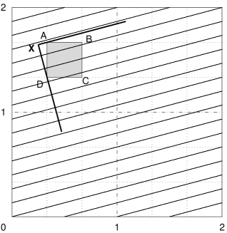
Figure 5: Ray $\gamma=[0,\alpha]$ with $\tan\alpha=4/15$

In this frame, the coordinates of $A,B,C$ and $D$ satisfy

$$A\,(0,\frac{\sin\alpha}{N});\quad B\,(\frac{\sin\alpha}{N},\frac{\sin\alpha+\cos\alpha}{N});\quad C\,(\frac{\sin\alpha+\cos\alpha}{N},\frac{\cos\alpha}{N});\quad D\,(\frac{\cos\alpha}{N},0).$$

The ray $\gamma$ is constituted of $p+q$ vertical segments. $R$ of them meet $K$ (see Figure 6). We note $x_{0},x_{1},\dots x_{R-1}$ their abscissa

$$\left\{\begin{array}[]{ll}x_{0}=r\in[0,\delta]\\ x_{i}=x_{0}+i\delta,\quad 0\leq i\leq R-1\end{array}\right..$$

Since $\frac{\sin\alpha+\cos\alpha}{N}=\frac{p+q}{2N}\delta>\delta$, there exists at least one segment in $K$ and $R\geq 1$.

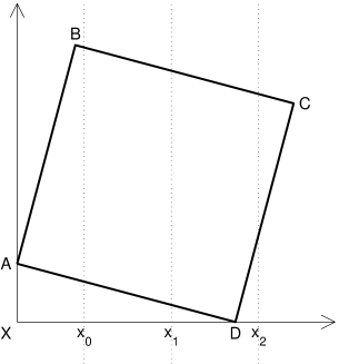
Figure 6: Vertical segments in the square $ABCD$

Let

$$\begin{array}[]{lllll}f_{1}(x)&=\cot\alpha\;x+\dfrac{\sin\alpha}{N}=\cot\alpha\,(x-\dfrac{\sin\alpha}{N})+\dfrac{\sin\alpha+\cos\alpha}{N}\;\text{ line }(AB)\\ f_{2}(x)&=-\tan\alpha\,(x-\dfrac{\sin\alpha}{N})+\dfrac{\sin\alpha+\cos\alpha}{N}\\ &=-\tan\alpha\,(x-\dfrac{\sin\alpha+\cos\alpha}{N})+\dfrac{\cos\alpha}{N}\;\text{ line }(BC)\\ g_{1}(x)&=-\tan\alpha\;x+\dfrac{\sin\alpha}{N}=-\tan\alpha\,(x-\dfrac{\cos\alpha}{N})\;\text{ line }(AD)\\ g_{2}(x)&=\cot\alpha\,(x-\dfrac{\cos\alpha}{N})=\cot\alpha\,(x-\dfrac{\sin\alpha+\cos\alpha}{N})+\dfrac{\cos\alpha}{N}\;\text{ line }(CD).\end{array}$$

and

$$f(x)=\left\{\begin{array}[]{llll}\dfrac{\sin\alpha}{N}&\text{if }x\leq 0\\ f_{1}(x)&\text{if }0\leq x\leq\frac{\sin\alpha}{N}\\ f_{2}(x)&\text{if }\frac{\sin\alpha}{N}\leq x\leq\frac{\sin\alpha+\cos\alpha}{N}\\ \dfrac{\cos\alpha}{N}&\text{if }x\geq\frac{\sin\alpha+\cos\alpha}{N}\end{array}\right.\text{and }g(x)=\left\{\begin{array}[]{llll}\dfrac{\cos\alpha}{N}&\text{if }x\leq 0\\ g_{1}(x)&\text{if }0\leq x\leq\frac{\cos\alpha}{N}\\ g_{2}(x)&\text{if }\frac{\cos\alpha}{N}\leq x\leq\frac{\sin\alpha+\cos\alpha}{N}\\ \dfrac{\cos\alpha}{N}&\text{if }x\geq\frac{\sin\alpha+\cos\alpha}{N}\end{array}\right..$$

Then

$$\int_{\mathbb{R}}f-g=\int_{0}^{\frac{\sin\alpha+\cos\alpha}{N}}(f(x)-g(x))dx=|K|=\frac{1}{N^{2}}$$

and

$$\frac{1}{L}\int_{0}^{L}\chi_{K}(\gamma(s))ds=\frac{\delta}{4}\sum_{i=0}^{R-1}f(x_{i})-g(x_{i}).$$

Let $k$ be the number of vertical segments which meet $[AB]$, i.e. the $k$ segments such that

$$r+(k-1)\delta\leq\frac{\sin\alpha}{N}\leq r+k\delta.$$

If $1\leq k\leq R-1$, if at least one segment meets $[AB]$ and if at least one segment meets $[BC]$ then, as one can see

$$\frac{1}{L}\sum_{i=0}^{R-1}f(x_{i}) =\frac{\delta}{4}\sum_{i=0}^{k-1}f_{1}(x_{i})+\frac{\delta}{4}\sum_{i=k}^{R-1}f_{2}(x_{i})$$

$$=\frac{1}{4}\sum_{i=0}^{k-1}\int_{x_{i}-\delta/2}^{x_{i}+\delta/2}f_{1}(x)dx+\frac{1}{4}\sum_{i=k}^{R-1}\int_{x_{i}-\delta/2}^{x_{i}+\delta/2}f_{2}(x)dx$$

$$=\frac{1}{4}\int_{r-\delta/2}^{r+(k-1/2)\delta}f_{1}(x)dx+\frac{1}{4}\int_{r+(k-1/2)\delta}^{r+(R-1/2)\delta}f_{2}(x)dx.$$ (3.1)

If $k=0$ or $k=R$, equation (3.1) remains true. Hence, in all cases

$$\begin{split}\frac{1}{L}\sum_{i=0}^{R-1}f(x_{i})&=\frac{1}{4}\int_{0}^{(p+q)\delta/2N}f(x)dx-\frac{1}{4}\int_{0}^{r-\delta/2}f_{1}(x)dx\\ &\qquad+\frac{1}{4}\int_{q\delta/2N}^{r+(k-1/2)\delta}(f_{1}(x)-f_{2}(x))dx+\frac{1}{4}\int_{(p+q)\delta/2N}^{r+(R-1/2)\delta}f_{2}(x)dx.\end{split}$$

In the same way, let $l$ be the number of segments which meet $[AD]$

$$r+(l-1)\delta\leq\frac{\cos\alpha}{N}\leq r+l\delta.$$

We obtain that, in all cases

$$\begin{split}\frac{1}{L}\sum_{i=0}^{R-1}g(x_{i})&=\frac{1}{4}\int_{r-\delta/2}^{r+(l-1/2)\delta}g_{1}(x)dx+\frac{1}{4}\int_{r+(l-1/2)\delta}^{r+(R-1/2)\delta}g_{2}(x)dx\\ &=\frac{1}{4}\int_{0}^{(p+q)\delta/2N}g(x)dx-\frac{1}{4}\int_{0}^{r-\delta/2}g_{1}(x)dx\\ &\qquad+\frac{1}{4}\int_{p\delta/2N}^{r+(l-1/2)\delta}(g_{1}(x)-g_{2}(x))dx+\frac{1}{4}\int_{(p+q)\delta/2N}^{r+(R-1/2)\delta}g_{2}(x)dx.\end{split}$$

Finally

$$\begin{split}\frac{1}{L}\int_{0}^{L}\chi_{K}(\gamma(s))ds-\frac{1}{4N^{2}}&=-\frac{1}{4}\int_{0}^{r-\delta/2}f_{1}-g_{1}+\frac{1}{4}\int_{q\delta/2N}^{r+(k-1/2)\delta}f_{1}-f_{2}\\ &\qquad+\frac{1}{4}\int_{p\delta/2N}^{r+(l-1/2)\delta}g_{1}-g_{2}+\frac{1}{4}\int_{(p+q)\delta/2N}^{r+(R-1/2)\delta}f_{2}-g_{2}\\ &=\frac{\tan\alpha+\cot\alpha}{8}\left[-(r-\delta/2)^{2}+(r+(k-1/2)\delta-q\delta/2N)^{2}\right.\\ &\qquad\left.+(r+(l-1/2)\delta-p\delta/2N)^{2}-(r+(R-1/2)\delta-(p+q)\delta/2N)^{2}\right].\end{split}$$

However, in this last equality, each of the four square terms is less than $\delta/2$ and $\tan\alpha+\cot\alpha=\dfrac{1}{\sin\alpha\,\cos\alpha}=\dfrac{4}{pq\delta^{2}}=\dfrac{L^{2}}{4pq}$ hence

$$\left|\frac{1}{L}\int_{0}^{L}\chi_{K}(\gamma(s))ds-\frac{1}{4N^{2}}\right|\leq\frac{1}{4pq}.$$ (3.2)

We now consider:

$$\omega_{T}=\bigcup_{(i,j)\in E}C_{i,j},$$

where $E$ is a subset of $\{1,2,\dots,2N\}^{2}$ and $\text{card}(E)=N^{2}|\omega_{T}|=4N^{2}|\omega|$ ; then

$$m(\gamma)=\frac{1}{L}\int_{0}^{L}\chi_{\omega_{T}}(\gamma(s))ds=\sum_{(i,j)\in E}\frac{1}{L}\int_{0}^{L}\chi_{C_{i,j}}(\gamma(s))ds.$$

Hence

$$m(\gamma)-|\omega|=\sum_{(i,j)\in E}\left(\frac{1}{L}\int_{0}^{L}\chi_{C_{i,j}}(\gamma(s))ds-\frac{1}{4N^{2}}\right).$$

This leads to

$$\left|\,m(\gamma)-|\omega|\,\right|\leq\frac{\text{card}(E)}{4pq}=\frac{N^{2}}{pq}|\omega|.$$

If the area of $\omega$ is greater than 1/2, let $\omega^{\prime}$ be the adherence of $\Omega-\omega$ which is also a finite union of squares $C_{i,j}$, Hence

$$\left|\frac{1}{L}\int_{0}^{L}\chi_{\omega^{\prime}}(\gamma(s))ds-(1-|\omega|)\,\right|\leq\frac{N^{2}}{pq}(1-|\omega|)$$

or

$$\frac{1}{L}\int_{0}^{L}\chi_{\omega^{\prime}}(\gamma(s))ds=1-\frac{1}{L}\int_{0}^{L}\chi_{\omega}(\gamma(s))ds.$$

Finally, we get $\left|\,m(\gamma)-|\omega|\,\right|\leq\dfrac{N^{2}}{pq}(1-|\omega|)$. $\square$

3.2 Representation of $\omega$

For convenience, consider the frame $(O,\vec{I},\vec{J})$ with $\vec{I}=\vec{i}/(2N)$ and $\vec{J}=\vec{j}/(2N)$. As a consequence, $\Omega$ is now the square $[0,N]^{2}$, and $T$ is the torus $[0,2N]^{2}$. The length of closed rays defined by $(p,q)$ ($p,q$ relatively prime) such that $\cos\alpha=p/\sqrt{p^{2}+q^{2}}$ and $\sin\alpha=q/\sqrt{p^{2}+q^{2}}$ must be modified. The period is now

$$L=2N\sqrt{p^{2}+q^{2}}$$

and $C_{i,j}$ is such that:

$$C_{i,j}=[i-1,i]\times[j-1,j].$$

Let us define the matrix $M$ $N\times N$ such that $M_{i,j}=1$ if $C_{j,i}\subset\omega$, and $M_{i,j}=0$ if $C_{j,i}\not\subset\omega$. With this notation, the matrix $M$ is a representation of $\omega$. As an example, if $\omega$ is as in Figure 7 then

$$M=\left(\begin{array}[]{cccccc}1&1&0&0&1&1\\ 1&1&1&1&0&1\\ 0&1&0&1&0&1\\ 0&0&0&0&1&1\\ 1&1&0&0&0&0\\ 0&1&1&0&0&0\\ \end{array}\right).$$

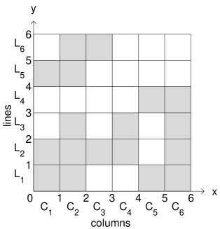
Figure 7: A domain $\omega$ for $N=6$

Let us also define the $2N\times 2N$ matrix $A$ such that $A_{i,j}=1$ if $C_{j,i}\subset\omega_{T}$, $A_{i,j}=0$ if $C_{j,i}\not\subset\omega_{T}$, i.e.

$$M_{i,j}=A_{i,j}=A_{2N+1-i,j}=A_{i,2N+1-j}=A_{2N+1-i,2N+1-j}.$$ (3.3)

3.3 Influent rays

Let $\gamma$ be a horizontal ray starting at $X_{0}=(x_{0},y_{0})$. Then,

$$m(\gamma)=\frac{1}{N}\sum_{j=1}^{N}M_{i,j}.$$

Assume that $y_{0}=k$ is an integer. Since each $C_{i,j}$ is closed,

$$m(\gamma)=\frac{1}{N}\sum_{j=1}^{N}(M_{k-1,j}+M_{k,j}).$$

Obviously, this ray does not realize the infimum in the definition of $g$. In the same way, for a vertical ray, only the numbers

$$\frac{1}{N}\sum_{i=1}^{N}M_{i,j},\quad 1\leq i\leq N.$$

must be considered. Now, let us deal with oblique rays and fix $\alpha$. Let us denote $\tan\alpha$ by $q/p$, where $p$ and $q$ are relatively prime integers.

Remark 3.1

One has to consider only the rays defined by $\gamma=[X_{0},\alpha]$ with $X_{0}\in T$ and $\alpha\in[0,\pi/2]$, i.e. $p\geq 0$ and $q\geq 0$.

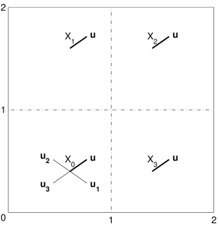
Figure 8: Starting points with $\alpha\in[0,\pi/2]$

Indeed, keeping the notations of Figure 8, the ray $\gamma^{1}=[X_{0},\overrightarrow{u_{1}}]$ is equivalent to $\tilde{\gamma}^{1}=[X_{1},\vec{u}]$. In the same way, the rays $\gamma^{2}=[X_{0},\overrightarrow{u_{2}}]$ and $\gamma_{3}=[X_{0},\overrightarrow{u_{3}}]$ are equivalent to $\tilde{\gamma}^{2}=[X_{2},\vec{u}]$ and $\tilde{\gamma}^{3}=[X_{3},\vec{u}]$.

Let us now study the influence of the starting point of rays. We have the following result

Proposition 3.1

Among oblique closed rays of angle $\alpha$, the ray which spends the least time in $\omega$ in average is a ray which meets a point with integer coordinates .

Proof : Let $B=(x_{0},y_{0})$ be a point of $T$ such that the ray $\gamma=[B,\alpha]$ does not meet a point with integer coordinates. Let us adopt the point of view of infinite plane and let $B_{0},B_{1},B_{2},\dots$ be the intersection points of $\gamma$ with the lattice $\mathbb{Z}+\mathbb{Z}$. A direct consequence of Theorem 1.1 is that $B_{0}B_{2N(p+q)}=L=2N\sqrt{p^{2}+q^{2}}$. $\vec{u}=(p\vec{i}+q\vec{j})/\sqrt{p^{2}+q^{2}}$ is the direction of the ray. Let $\vec{n}=(-q\vec{i}+p\vec{j})/\sqrt{p^{2}+q^{2}}$ be such that $(\vec{u},\vec{n})$ is a direct orthonormal frame. For a point $P=(k,l)$ with integer coordinates, let us compute the algebraic distance to the ray $\gamma$

$$d(P,\gamma)=\overrightarrow{BP}.\vec{n}=\frac{pl-qk-(py_{0}-qx_{0})}{\sqrt{p^{2}+q^{2}}}.$$

There exists a point $A$ with integer coordinates and which verifies:

$$d(A,\gamma)=\min\{d(P,\gamma)|P\text{ has integer coordinates and }d(P,\gamma)>0\}.$$

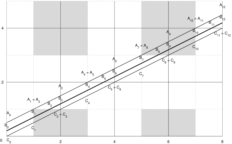
Figure 9: Case of a ray which does not meet any point with integer coordinates

Let $A_{i}$ be the intersection point of the line meeting $A$ and directed by $\vec{u}$ (the points $A$ solutions of the minimization problem above are clearly on a same line directed by $\vec{u}$) and the line belonging to the lattice $\mathbb{Z}+\mathbb{Z}$ which contains $B_{i}$ (see Figure 9 for the case $N=2$). In the same way, there exists $C$ with integer coordinates which satisfies

$$d(C,\gamma)=\min\{d(P,\gamma)|P\text{ has integer coordinates and }d(P,\gamma)<0\}.$$

Let us note $C_{i}$ the intersection of the line meeting $C$ and directed by $\vec{u}$ and the line belonging to the lattice $\mathbb{Z}+\mathbb{Z}$ which contains $B_{i}$ (see Figure 9).
There are three oblique rays of angle $\alpha$ $\gamma_{A}=[A_{0},\alpha]$, $\gamma_{B}=[B,\alpha]=[B_{0},\alpha]$ and $\gamma_{C}=[C_{0},\alpha]$. According to the definitions of $A$ and $C$, the segments $[A_{i}\,A_{i+1}]$, $[B_{i}\,B_{i+1}]$ and $[C_{i}\,C_{i+1}]$ belong to the same square $C_{k,l}$. We define $\varepsilon_{k}=1$ if $[B_{k}\,B_{k+1}]\subset\omega_{T}$, $\varepsilon_{k}=0$ if $[B_{k}\,B_{k+1}]\not\subset\omega_{T}$. Then, if

$$m(\gamma_{B})=\frac{1}{L}\int_{[B_{0}B_{2N(p+q)}]}\chi_{\omega_{T}}=\frac{1}{L}\sum_{k=1}^{2N(p+q)}\varepsilon_{k}\,B_{k-1}B_{k},$$

we have:

$$m(\gamma_{A})=\frac{1}{L}\sum_{k=1}^{2N(p+q)}\varepsilon_{k}\,A_{k-1}A_{k}\quad\text{and}\quad m(\gamma_{C})=\frac{1}{L}\sum_{k=1}^{2N(p+q)}\varepsilon_{k}\,C_{k-1}C_{k}.$$

These three rays are parallel. Hence, there exists $t\in(0,1)$ such that for all $i$, $B_{i}$ is the barycenter of $(A_{i},t)$ and $(C_{i},1-t)$. If the quadrilateral $A_{i}\,A_{i+1}\,C_{i}\,C_{i+1}$ is a trapezium (or in the degenerate case a rectangular triangle), Thales’ theorem implies that $B_{i}B_{i+1}=t\,A_{i}A_{i+1}+(1-t)\,C_{i}C_{i+1}$. If the quadrilateral is a parallelogram, this inequality remains valid because the three lengths are equal. As a consequence, we have

$$m(\gamma_{B})=tm(\gamma_{A})+(1-t)m(\gamma_{C}).$$

The minimum of the three quantities $m(\gamma_{A})$, $m(\gamma_{B})$ and $m(\gamma_{C})$ is attained for one of the two rays $\gamma_{A}$ ou $\gamma_{C}$. This shows that $\gamma$ cannot be the minimum in the set of oblique closed rays. $\square$

It remains to find the angles $\alpha$ we need to consider among the rays which meet a point with integer coordinates. In the flat torus $T=[0,\,2N]^{2}$, there are $4N^{2}$ possible starting points. However, the ray $\gamma=[(x_{0},y_{0}),\alpha]$ with $(x_{0},y_{0})\in\mathbb{N}^{2}$ meets $2N$ points with integer coordinates. Indeed, $\gamma$ meets the point $(x_{1},y_{1})$ if and only if there exists $\lambda\in[0,2N)$ such that

$$\left\{\begin{array}[]{ll}x_{1}=x_{0}+\lambda p\;\;[2]\\ y_{1}=y_{0}+\lambda q\;\;[2]\end{array}\right..$$

Therefore, the points belonging to $\gamma$ and with integer coordinates are exactly the $2N$ points obtained for $\lambda=0,1,\dots,2N-1$. There exist at least $2N$ rays which meet a point with integer coordinates.

Proposition 3.2

Let $d$ be the G.C.D. of $p$ and $2N$, let $d^{\prime}$ be such that $d\,d^{\prime}=2N$. Then, the $2N$ rays of angle $\alpha$ starting at $(i,j)$ with $0\leq i\leq d-1$ and $0\leq j\leq d^{\prime}-1$ meet one and only one time all the points of $T$ with integer coordinates.

Proof : Let $p^{\prime}$ be such that $d\,p^{\prime}=p$. We note that $p^{\prime}$ and $d^{\prime}$ are relatively prime. Let also $\gamma_{1}$ and $\gamma_{2}$ be the rays starting respectively at $A$ and $B$ with integer coordinates $(k_{1},k_{2})$ and $(k_{3},k_{4})$ (with $0\leq k_{1},\,k_{3}\leq d-1$ and $0\leq k_{2},\,k_{4}\leq d^{\prime}-1$ ). There exists a point $C\in\gamma_{1}\cap\gamma_{2}$ with integer coordinates if and only if there exist four integer numbers $\lambda,\mu,n$ and $m$ such that

$$\left\{\begin{array}[]{ll}x=k_{1}+\lambda p=k_{3}+\mu p+2Nn\\ y=k_{2}+\lambda q=k_{4}+\mu q+2Nm\end{array}\right..$$

Therefore, $k_{1}-k_{3}=(\mu-\lambda)p+2Nn$ and $k_{1}-k_{3}$ is divisible by $d$. Since $-(d-1)\leq k_{1}-k_{3}\leq d-1$, we have $k_{1}=k_{3}$ and $(\mu-\lambda)p=-2Nn$. As a consequence, $(\mu-\lambda)p^{\prime}=-d^{\prime}n$ and since $p^{\prime}$ and $d^{\prime}$ are relatively prime, $(\mu-\lambda)=kd^{\prime}$, where $k\in\mathbb{Z}$. In the same way, $k_{2}-k_{4}=(\mu-\lambda)q+2Nm=kd^{\prime}q+2Nm$. Hence $k_{2}-k_{4}$ is divisible by $d^{\prime}$. Since $-(d^{\prime}-1)\leq k_{2}-k_{4}\leq d^{\prime}-1$, we have $k_{2}=k_{4}$ and $\gamma_{1}=\gamma_{2}$. $\square$

3.4 The algorithm

In this section, we give a method to compute explicitly $g$ when $\omega$ is a finite union of squares $C_{i,j}$. At first, according to Propositions 1.1 and 3.1, the study can be restricted to closed rays starting at a point with integer coordinates.
The user of the program must input the matrix $M$ which represents $\omega$ and the value of a parameter $PQmax$ which avoids infinite loops (this problem never appeared until now).

The algorithm is the following

1. Compute the minimum $g$ of the $2N$ numbers

   $$\frac{1}{N}\sum_{i=1}^{N}M_{i,j}\;\text{ and }\;\frac{1}{N}\sum_{j=1}^{N}M_{i,j},$$

   which corresponds to the minimum of $m(\gamma)$ when $\gamma$ is a vertical or horizontal ray.

2. From the matrix $M$, build the matrix $A$ defined in (3.3).

3. For all $(p,q)$ such that $p\geq 1$, $q\geq 1$, $p+q\leq 2N$ and $p$ and $q$ relatively prime, compute the number (the way to compute $m_{p,q}$ is explained below)

   $$m_{p,q}=\min_{X\in\{1,2,\dots,2N\}^{2}}\{m(\gamma)|\gamma=[X,\arctan q/p]\}.$$ (3.4)

   Then $g\leftarrow\min\{g,m_{p,q}\}.$

4. If at this step $g=|\omega|$, the user inputs the parameter $PQmax$ which corresponds to the greatest product $pq$ which will be considered ; in the other cases $PQmax=E(\frac{N^{2}}{|\omega|-g}\min\{|\omega|,1-|\omega|\})+1$.

5. Find all the $(p,q)$ relatively prime such that $p\geq 1$, $q\geq 1$, $p+q>2N$, $pq\leq PQmax$. Sort these couples from the lowest product $pq$ to the greatest one. This gives a list $L$ containing $n$ couples.

6. $i\leftarrow 1$ and as long as $|\omega|-g\geq\frac{N^{2}}{pq}\min\{|\omega|,1-|\omega|\}$ and $i\leq n$,

   $$g\leftarrow\min\{g,m_{p,q}\}\;\text{ and }\;i\leftarrow i+1,$$

   where $(p,q)$ is the i-th couple of $L$ and $m_{p,q}$ is defined above (see (3.4)).

7. Finally

   • if at the end of this loop, $g=|\omega|$, then

     $$|\omega|-\frac{N^{2}}{PQmax}\min\{|\omega|,1-|\omega|\}\leq g(\omega)\leq|\omega|.$$

     This means that one of the following cases occurs; $g(\omega)=|\omega|$, or too few families of rays have been considered.

   • if $g\not=|\omega|$, according to Theorem 3.1, $g(\omega)$ is equal to $g$.

We now present the method of computation defined in (3.4) for two relatively prime integers $p\geq 1$, $q\geq 1$. At first, let us consider the ray $\gamma_{0}=[0,\arctan q/p]$ and let us study the way to compute $m(\gamma_{0})$. Its period is $L=2N\sqrt{p^{2}+q^{2}}$ and between the instants $t=0$ and $t=L$, it meets $2N(p+q-1)+1$ points which have at least one integer coordinate. Let $P_{1}$,…, $P_{2N(p+q-1)+1}$ be these points (see Figure 10). Remember that $P_{l(p+q-1)+1}$, $1\leq l\leq 2N$ have integer coordinates.

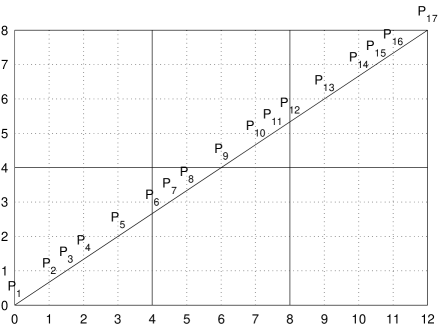
Figure 10: Ray $\gamma_{0}$, for $N=2$, $p=3$ and $q=2$

Let $(i_{k})$, $(j_{k})$ and $(\varepsilon_{k})$ be the three other finite sequences ($1\leq k\leq 2N(p+q-1)$) defined by

$$P_{k}P_{k+1}\subset[i_{k},i_{k}+1]\times[j_{k},j_{k}+1]$$

and

$$\varepsilon_{k}=\left\{\begin{array}[]{ll}1\text{ if }[i_{k},i_{k}+1]\times[j_{k},j_{k}+1]\subset\omega\\ 0\text{ if not }\end{array}\right..$$

Then, $m(\gamma_{0})=\frac{1}{L}\sum_{k=1}^{2N(p+q-1)}\varepsilon_{k}P_{k}P_{k+1}$, the computation of $m(\gamma_{0})$ is equivalent to the computation of the sequences $(P_{k}P_{k+1})$, $(i_{k})$ and $(j_{k})$.

$\bullet$ Computation of the lengths $P_{k}P_{k+1}$
At first, note that it suffices to compute the lengths $P_{k}P_{k+1}$ for $1\leq k\leq p+q-1$. Indeed, $\overrightarrow{P_{k+(p+q-1)}P_{k}}=p\vec{i}+q\vec{j}$, hence the sequence $(P_{k}P_{k+1})$ is periodic of period $p+q-1$. Since $p$ and $q$ are relatively prime, $P_{1}$ and $P_{p+q-1}$ do not have integer coordinates.

Then, the equations of the ray $\gamma_{0}$ are $x=pt/\sqrt{p^{2}+q^{2}}$ and $y=qt/\sqrt{p^{2}+q^{2}}$. It meets the vertical lines defined by $x=i$ at instants $t_{i}=i\sqrt{p^{2}+q^{2}}/p$ at points $(i,iq/p)$ and the horizontal lines defined by $y=j$ at instants $t^{\prime}_{j}=j\sqrt{p^{2}+q^{2}}/q$ and at points $(jp/q,j)$.
Let us then define the list $V^{1}$ by

$$V^{1}=\{t^{\prime}_{j},1\leq j\leq q-1\}\cup\{t_{i},1\leq i\leq p-1\}.$$

Let $V^{2}$ be the list obtained from $V^{1}$ by sorting its elements in increasing order. Let also $\sigma$ be the permutation of $\{1,2,\dots,p+q-2\}$ such that

$$V^{2}=\sigma(V^{1})=\{V^{1}_{\sigma(1)},V^{1}_{\sigma(2)},\dots,V^{1}_{\sigma(p+q-2)}\}.$$

Let $V^{3}$ and $V^{4}$ be defined by

$$V^{3}=\{0\}\cup V^{2}\cup\{\sqrt{p^{2}+q^{2}}\}\;\text{ and }\;V^{4}=\{V^{3}_{2}-V^{3}_{1},V^{3}_{3}-V^{3}_{2},\dots,V^{3}_{p+q}-V^{3}_{p+q-1}\}.$$

Finally, let $V$ be defined by

$$\begin{array}[]{cc}V=&\underbrace{V^{4}\cup V^{4}\cup\dots\cup V^{4}}\\ &2N\text{ times}\end{array},$$

then for all $k$, $1\leq k\leq 2N(p+q-1)$ $P_{k}P_{k+1}=V_{k}$ and

$$m(\gamma_{0})=\frac{1}{2N\sqrt{p^{2}+q^{2}}}\sum_{k=1}^{2N(p+q-1)}\varepsilon_{k}V_{k}.$$

As an important remark, it may be convenient to work with $pq/\sqrt{p^{2}+q^{2}}\,.V$ instead of $V$. Thus, $V_{1}=\{pj,1\leq j\leq q-1\}\cup\{qi,1\leq i\leq p-1\}$, $V_{3}=\{0\}\cup V^{2}\cup\{pq\}$ and hence, the elements of $V$ are all integer numbers. $m(\gamma_{0})$ is then given by

$$m(\gamma_{0})=\frac{\sum_{k=1}^{2N(p+q-1)}\varepsilon_{k}V_{k}}{2Npq}.$$

As a consequence, $m(\gamma_{0})$ is a rational number whose denominator and numerator are explicitly known.

$\bullet$ Computation of the sequences $(i_{k})$ and $(j_{k})$
Let $I^{1}$ and $J^{1}$ be the two following lists

$$\begin{array}[]{cccccc}I^{1}=&\{\underbrace{1,1,\dots,1},&\underbrace{0,0,\dots,0}\}&\;\text{ and }\;J^{1}=&\{\underbrace{0,0,\dots,0},&\underbrace{1,1,\dots,1}\}\\ &q-1\text{ times}&p-1\text{ times}&&q-1\text{ times}&p-1\text{ times}\end{array}.$$

This means that the numbers 1 which appear in the sequence $I^{1}$ correspond to the points $P_{k}$ which belong to horizontal lines and the numbers 1 of the sequence $J^{1}$ correspond to the points $P_{k}$ belonging to vertical lines. From these two lists and from the permutation $\sigma$, we define

$$I^{2}=\sigma(I^{1})=\{I^{1}_{\sigma(1)},I^{1}_{\sigma(2)},\dots,I^{1}_{\sigma(p+q-2)}\}\;\text{ and }\;J^{2}=\sigma(J^{1})=\{J^{1}_{\sigma(1)},J^{1}_{\sigma(2)},\dots,J^{1}_{\sigma(p+q-2)}\}$$

and also

$$I^{3}=\left\{0,I^{2}_{1},\sum_{k=1}^{2}I^{2}_{k},\dots,\sum_{k=1}^{p+q-2}I^{2}_{k}\right\}\;\text{ and }\;J^{3}=\left\{0,J^{2}_{1},\sum_{k=1}^{2}J^{2}_{k},\dots,\sum_{k=1}^{p+q-2}J^{2}_{k}\right\}.$$

Finally, we set

$$I=I^{3}\cup(p+I^{3})\cup\dots\cup([2N-1]p+I^{3})\;\text{ and }J=J^{3}\cup(q+J^{3})\cup\dots\cup([2N-1]q)+J^{3}.$$

Then, for all $k$, $1\leq k\leq 2N(p+q-1)$, $i_{k}=1+I_{k}$ and $j_{k}=1+J_{k}$.
Let us introduce the matrix $A$ defined from $M$ in (3.3) and a function $r$ defined over integers by

$$r(k)\in\{1,2,\dots,2N\}\;\text{ and }\;\exists\,l\in\mathbb{Z}\,|\,k=2N.l+r(k).$$

Then, for all $k$, $1\leq k\leq 2N(p+q-1)$, $\varepsilon_{k}=A_{r(i_{k}),r(j_{k})}=A_{r(1+I_{k}),r(1+J_{k})}$.

There are two reasons why we consider all rays of angle $\arctan q/p$ at the same time in the computation of $m_{p,q}$. First, all these rays have the same sequence $V_{k}$. In addition, let $\gamma=[X_{0},\arctan(\frac{q}{p})]$ where $X_{0}=(x_{0},y_{0})$ has integer coordinates. Then, the sequences $(i_{k})$ and $(j_{k})$ of $\gamma$ can be computed from the lists $I_{k}$ and $J_{k}$ by the formula: $i_{k}=1+x_{0}+I_{k}$ and $j_{k}=1+x_{0}+J_{k}$.

For two relatively prime integers $p\geq 1$ and $q\geq 1$, the number $m_{p,q}$ can be computed in the following way

1. compute the G.C.D. $d$ of $p$ and $2N$ and from Proposition 3.2, the $2N$ starting points with integer coordinates that must be considered are known. Let us note $X_{1},X_{2},\dots,X_{2N}$ and $Y_{1},Y_{2},\dots,Y_{2N}$ their coordinates.

2. Compute the three lists of $2N(p+q-1)$ elements $V_{k}$, $I_{k}$ and $J_{k}$ defined above.

3. $m_{p,q}$ is then the minimum of the $2N$ numbers

   $$\frac{\sum_{l=1}^{2N(p+q-1)}A_{r(1+X_{k}+I_{l}),r(1+Y_{k}+J_{l})}\,V_{l}}{2Npq}.$$

   All these quotients have the same denominator and hence, are easy to compare by looking at their numerator. Finally, this gives the explicit value of $m_{p,q}$.

We now present the results obtained with our algorithm for explicit domains $\omega$.

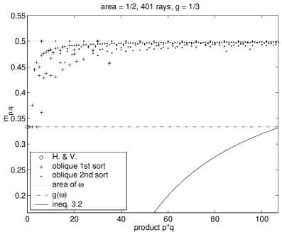
Figure 11: An example of computation of $g(\omega)$

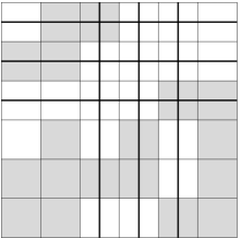
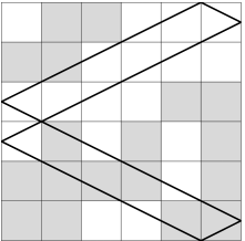
a.  b.
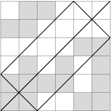
c.  d.

Figure 12: Minimizing rays : $m(\gamma)=g(\omega)=1/3$

Figure 13: Minimizing ray : $m(\gamma)=g(\omega)=111/560$

As an example, for the computation of $g(\omega)$ for the domain $\omega$ of Figure 7, the minimum for vertical and horizontal rays is $g=1/3$ and there are 45 families of oblique rays of first kind (i.e. the rays of part 3 in algorithm). Among these rays, there exists $\gamma$ such that $m(\gamma)=1/3$ but there is no $\gamma$ such that $m(\gamma)<1/3$. At this step, the value of $g$ is $1/3$. There are also 344 families of oblique rays of second kind (corresponding to part 5 of algorithm). None of them satisfies $m(\gamma)=1/3$. We obtain $g(\omega)=1/3$.

Figure 11 presents the values of $m_{p,q}$ as a function of $pq$ and presents also inequality of Theorem 3.1. Note that this inequality is not optimal for this particular domain. However, (3.2) is optimal for a unique square $C_{i,j}$. This shows that the error comes from the summation of inequalities (3.2) for all the squares of $\omega_{T}$. Nevertheless, it is useful because it certifies that the value of $g(\omega)$ is exact.

There exist 10 rays which satisfy $m(\gamma)=g(\omega)$; six vertical or horizontal rays (more precisely six families of vertical or horizontal rays). They are represented on Figure 12.a. There are also two rays of angle $\pi/4$ represented on Figure 12.b, one ray of angle $\arctan 1/2$ represented on Figure 12.c, and also the ray $\gamma=[0,\arctan 1/4]$ represented on Figure 12.d.

The domain $\omega$ of Figure 13 of area $|\omega|=29/100$ is represented here to show that intuition can be false. Indeed, consider only vertical rays, horizontal rays and closed rays of small period. The intuition says that $g(\omega)=1/5$. However, the ray $\gamma=[0,\arctan 8/7]$ is such that $m(\gamma)=111/560$ (note that 1/5=112/560), that is the exact value of $g(\omega)$ as shown by the complete computation.

4 Appendix : proof of Theorem 2.1

First, it is clear that

$$g(\omega)\leq g^{\prime}(\omega).$$ (4.1)

Indeed, for all $\gamma^{\prime}\in\mathcal{C}$ and all $t>0$, $m(\gamma_{t}^{\prime})\geq\inf_{\gamma\in\mathcal{C}}m(\gamma_{t})$. Hence,

$$m(\gamma^{\prime})=\limsup_{t\to+\infty}m(\gamma^{\prime}_{t})\geq\limsup_{t\to+\infty}\inf_{\gamma\in\mathcal{C}}m(\gamma_{t})=g(\omega).$$

Since this equality is true for all $\gamma^{\prime}\in\mathcal{C}$, this shows (4.1).

Let us prove that

$$g(\omega)\geq g^{\prime}(\omega).$$ (4.2)

Let us fix $\epsilon>0$ and choose a sequence $(\gamma^{n})_{n}\subset\mathcal{C}$ and a sequence $(t_{n})_{n}$ which tends to $+\infty$ such that

$$\lim_{n\to+\infty}m(\gamma^{n}_{t_{n}})=g(\omega).$$ (4.3)

For all $n\in\mathbb{N}$, there exist $X_{n}\in\Omega$ and $\theta_{n}\in[0,2\pi[$ such that $\gamma^{n}=[X_{n},\theta_{n}]$. Up to a subsequence, we can assume that there exists $(X_{0},\theta)\in\overline{\Omega}\times[0,2\pi]$ such that

$$\lim_{n}X_{n}=X_{0}\hbox{ and }\lim_{n}\theta_{n}=\theta.$$

We claim that there exists $L>0$ such that

$$m([y,\theta]_{L})\geq g^{\prime}(\omega)-\epsilon\hbox{ for all }y\in\Omega.$$ (4.4)

If $\tan(\theta)\in\mathbb{R}\backslash\mathbb{Q}$, then set $L=t_{0}$, where $t_{0}$ is as in Proposition 1.1. Indeed, together with relation (2.1),

$$m([y,\theta]_{L})\geq|\omega|-\epsilon\geq g^{\prime}(\omega)-\epsilon.$$

If $\tan(\theta)\in\mathbb{Q}$ or if $\tan(\theta)=\infty$, the ray $[y,\theta]$ is periodic and the period $T$ does not depend on $y\in\Omega$. Hence,

$$m([y,\theta]_{L})=m([y,\theta])\geq g^{\prime}(\omega).$$

Thus, let us set $L=T$. Clearly, $t_{n}$ can be assumed to be a multiple of $L$. Indeed, replacing $t_{n}$ by $t_{n}+s_{n}$ (where $|s_{n}|\leq L$) does not change the limit of $m(\gamma^{n}_{t_{n}})$. Now, assume that $\theta_{n}=\theta$. If $\tan(\alpha)\in\mathbb{Q}$ or if $\tan(\alpha)=\infty$, then clearly $\lim_{n}m(\gamma^{n}_{t_{n}})-m(\gamma^{n})=0$. If $\tan(\alpha)\in\mathbb{R}\backslash\mathbb{Q}$, this relation follows from Proposition 1.1. Then, by relation (4.3), it follows that

$$g(\omega)\geq\liminf_{n}m(\gamma^{n})\geq g^{\prime}(\omega).$$

This proves (4.2). Hence, we can assume that

$$\theta_{n}\not=\theta.$$ (4.5)

Now, let us define, for $k\in\{0,...,\frac{t_{n}}{L}-1\}$, $X_{k,n}=\gamma^{n}(kL)$ and $\gamma^{k,n}(t)=\gamma^{n}(kL+t)$ for $t\in[0,L]$. Let us define also ${\gamma}^{k,n,s}$ as the unique trajectory of length $L$ and slope $\theta$ such that ${\gamma}^{k,n,s}(s)=\gamma^{k,n}(s)$ and

$$A_{k,n}=\bigcup_{s\in[0,L]}{\gamma}^{k,n,s}.$$

\begin{picture}(0.0,0.0)\end{picture}

Now, we prove that

Step 1

There exists a sequence $(k_{n})_{n}$ such that

$$|A_{k_{n},n}\cap\partial\omega|\leq\epsilon\hbox{ and }m(\gamma^{k_{n},n})\leq g(w)+\epsilon$$

for all $n$ large enough. Here, $|A_{k_{n},n}\cap\partial\omega|$ denotes the length of the curve $A_{k_{n},n}\cap\partial\omega$.

In the following, the length of any curve $C$ will be denoted by $|C|$. Let

$$\mathcal{K}_{n}=\left\{k\in\{0,...,\frac{t_{n}}{L}-1\}\hbox{ s.t. }m(\gamma^{k,n})\leq g(w)+\epsilon\right\}.$$

Set

$$\mathcal{M}=\bigcap_{m\in\Delta}\left(\overline{\bigcup_{n\geq m;k\in\mathcal{K}_{n}}X_{k,n}}\right)$$

and

$$\tilde{\mathcal{M}}=\bigcap_{m\in\Delta}\left(\overline{\bigcup_{n\geq m;k\in\mathcal{K}_{n}}\gamma^{k,n}}\right).$$

For $X\in\mathcal{M}$, let $\gamma_{X}$ denote the trajectory of length $L$ and slope $\theta$ such that $\gamma_{X}(0)=X$. Note that $\mathcal{M}$ and $\tilde{\mathcal{M}}$ are not empty. Otherwise, $\mathcal{K}_{n}$ would be empty too and we would have $m(\gamma^{k,n})\geq g(\omega)+\epsilon$ for all $n\geq n_{0}$ and forall $k$. Thus, we would have $m(\gamma^{n}_{t_{n}})\geq g(\omega)+\epsilon$ that contradicts (4.3). Now, we prove that

$$\tilde{\mathcal{M}}=\bigcup_{y\in\mathcal{M}}\gamma_{y}.$$ (4.6)

Take a sequence $(X_{l_{n},n})_{n}$ such that $\lim_{n}X_{l_{n},n}=y\in\mathcal{M}$. Then, for all $t\in[0,L]$, $\lim\gamma^{l_{n},n}(t)=\gamma_{y}(t)$. We obtain that

$$\bigcup_{y\in\mathcal{M}}\gamma_{y}\subset\tilde{\mathcal{M}}.$$

Conversely, if $z\in\tilde{\mathcal{M}}$ then there exist two sequences $(l_{n})_{n}$ such that $l_{n}\in\mathcal{K}_{n}$ and $(s_{n})_{n}\subset[0,L]$ such that $z=\lim_{n}\gamma^{l_{n},n}(s_{n})$. Up to a subsequence, we can assume that there exist $y\in\mathcal{M}$ and $s\in[0,L]$ such that $\lim_{n}X_{k_{n},n}=y$ and $\lim_{n}s_{n}=s$. As one can check, this implies that $z=\lim_{n}\gamma^{k_{n},n}(s)=\gamma_{y}(s)$ and therefore

$$\tilde{\mathcal{M}}\subset\bigcup_{y\in\mathcal{M}}\gamma_{y}.$$

This proves (4.6).

We now distinguish two cases.

First, assume that there exists an infinite sequence $(y_{n})_{n}$ in $\mathcal{M}$ such that $\gamma_{y_{n}}\cap\gamma_{y_{n^{\prime}}}=\emptyset$ if $n\not=n^{\prime}$. Since $|\partial\omega|$ is finite, one can choose $y\in\mathcal{M}$ ($y$ is one of the $y_{n}$) such that $|\gamma_{y}\cap\partial\omega|\leq\frac{\epsilon}{2}$. Otherwise, for all $n$, $|\partial\omega\cap\gamma_{y_{n}}|\geq\frac{\epsilon}{2}$ and hence, since $\gamma_{y_{n}}\cap\gamma_{y_{n^{\prime}}}=\emptyset$, we would have

$$+\infty=\sum_{n}|\partial\omega\cap\gamma_{y_{n}}|=\left|\left(\cup_{n}\gamma_{y_{n}}\right)\cap\partial\omega\right|\leq|\partial\omega|.$$

This is false. The definition of $\mathcal{M}$ implies that there exists a sequence $(k_{n})_{n}$ such that $y=\lim_{n}X_{k_{n},n}$ with $k_{n}\in\mathcal{K}_{n}$. Clearly, for all $t\in[O,L]$,

$$\lim_{n}\gamma^{k_{n},n}(t)=\gamma_{y}(t).$$ (4.7)

Set $B_{n}=\overline{\bigcup_{m\geq n}A_{k_{n},n}}$. Obviously, $B_{n}$ is a decreasing sequence of sets. We recall that

$$A_{k_{n},n}=\bigcup_{s\in[0,L]}\gamma^{k_{n},n,s}$$

By construction, for all $t\in[0,L]$, $\gamma^{k_{n},n,s}(t)=\gamma_{y}(t)$. This implies that $\bigcap_{n\in\mathbb{N}}B_{n}=\gamma_{y}$. Since $|\gamma_{y}\cap\partial\omega|\leq\frac{\epsilon}{2}$, for all $n$ large enough, we have $|B_{n}\cap\partial\omega|\leq\epsilon$. Since $A_{k_{n},n}\subset B_{n}$ and since $k_{n}\in\mathcal{K}_{n}$, this proves Step 1 in this case.

Now, assume, for all infinite sequences $(y_{n})_{n}$ in $\mathcal{M}$, there exists $n\not=n^{\prime}$ such that $\gamma_{y_{n}}\cap\gamma_{y_{n^{\prime}}}\not=\emptyset$. Clearly, this case occurs if $\mathcal{M}$ is finite. Then, choose a finite set $\{y_{1},\cdots,y_{k}\}\subset\mathcal{M}$  such that $\gamma_{y_{n}}\cap\gamma_{y_{n^{\prime}}}=\emptyset$ if $n\not=n^{\prime}$ and assume that $k$ is maximal. This means that for all $y\in\mathcal{M}$, there exists $n\in\{1,...,k\}$ such that $\gamma_{y}\cap\gamma_{y_{n}}\not=\emptyset$ (otherwise the set $\{y,y_{1},\cdots,y_{k}\}$ would have the above property and $k$ would not be maximal). Since $|\gamma_{y}|=L$, we have: $\gamma_{y}\subset\gamma_{y_{n}}^{\prime}$ where $\gamma_{y_{n}}^{\prime}$ is the trajectory of length $3L+2$ and slope $\theta$ such that $\gamma_{y_{n}}^{\prime}(L+1)=\gamma_{y_{n}}(0)$. Note that instead of $\gamma_{y_{n}}^{\prime}$, one could have considered trajectories of length $3L$. We need to consider trajectories strictly greater than $3L$ to get relation (4.10) below. For simplicity, we choose $3L+2$. Using (4.6), we see that

$$\tilde{\mathcal{M}}\subset\bigcup_{n=1}^{k}\gamma_{y_{n}}^{\prime}.$$ (4.8)

Let $n$ be fixed. Let

$$A_{n}=\left\{t\in[0,t_{n}]\left|\gamma^{n}(t)\in\bigcup_{m=1}^{k}\gamma_{y_{m}}^{\prime}\right.\right\}$$

The set $\bigcup_{m=1}^{k}\gamma_{y_{m}}^{\prime}$ is a finite union of disjoint trajectories of finite length and slope $\theta$. Moreover, $\theta_{n}\not=\theta$ (see (4.5)). Hence, $A_{n}$ is a discrete set of points. Since $\bigcup_{m=1}^{k}\gamma_{y_{m}}^{\prime}$ is closed, $A_{n}$ is closed too. This shows that $A_{n}$ is finite. Let now $t_{1},t_{2}\in A_{n}$ with $t_{1}<t_{2}$. As one can check, there exists $\alpha>0$ independent of $n$ such that if $t\leq\alpha{|\theta_{n}-\theta|}^{-1}$, $\gamma^{n}(t_{1}+t)\not\in\bigcup_{m=1}^{k}\gamma_{y_{m}}^{\prime}$. Indeed, $\bigcup_{m=1}^{k}\gamma_{y_{m}}^{\prime}$ is a finite union of segments of slope $\theta$. Then, it is clear that the trajectory $\gamma_{n}$, whose slope is $\theta_{n}$, meets two different segments of $\bigcup_{m=1}^{k}\gamma_{y_{m}}^{\prime}$ in a time proportional to the difference $|\theta_{n}-\theta|$ of the slopes. Hence $t_{2}-t_{1}\geq\alpha{|\theta_{n}-\theta|}^{-1}$. This proves that

$$\#A_{n}\leq\frac{t_{n}}{\alpha}|\theta_{n}-\theta|.$$ (4.9)

Moreover,

$$m(\gamma^{n}_{t_{n}})=\frac{1}{t_{n}}\int_{0}^{t_{n}}\mathcal{X}_{\omega}(\gamma^{n}_{t_{n}}(t))dt=\frac{L}{t_{n}}\sum_{l=1}^{\frac{t_{n}}{L}-1}\frac{1}{L}\int_{lL}^{(l+1)L}\mathcal{X}_{\omega}(\gamma^{n}_{t_{n}}(t))dt=\frac{L}{t_{n}}\sum_{l=1}^{\frac{t_{n}}{L}-1}m(\gamma^{l,n}).$$

From the definition of $K_{n}$, we write that for $l\in\mathcal{K}_{n}$ we have $m(\gamma^{l,n})\geq 0$ and we know that for $l\in\{0,...,\frac{t_{n}}{L}-1\}\backslash\mathcal{K}_{n}$, we have $m(\gamma^{l,n})\geq g(\omega)+\epsilon$. We obtain that

$$m(\gamma^{n}_{t_{n}})\geq\frac{L}{t_{n}}\#\left(\{0,...,\frac{t_{n}}{L}-1\}\backslash\mathcal{K}_{n}\right)(g(\omega)+\epsilon)=\frac{L}{t_{n}}\left(\frac{t_{n}}{L}-\#\mathcal{K}_{n}\right)(g(\omega)+\epsilon).$$

Since $\lim_{n}m(\gamma^{n}_{t_{n}})=g(\omega)$, t

$$\#\mathcal{K}_{n}\geq ct_{n}$$

where $c>0$ is independent of $n$. It follows from (4.9) that we can choose $k_{n}\in\mathcal{K}_{n}$ such that $[k_{n}L,(k_{n}+1)L]\cap A_{n}=\emptyset$. Hence, $\gamma^{k_{n},n}\cap\bigcup_{m=1}^{k}\gamma_{y_{m}}^{\prime}=\emptyset$. We can assume that $\lim_{n}X_{k_{n},n}=y\in\mathcal{M}$. Then, for all $t\in[0,L]$, we have: $\lim_{n}\gamma^{k_{n},n}(t)=[y,\theta](t)$. Since $\gamma_{y_{m}}^{\prime}$ has been chosen such that their length is $3L+2$, there exists an $m$ such that

$$[y,\theta]_{L}\subset\gamma_{y_{m}}^{\prime}$$ (4.10)

with $[y,\theta](0)\not=\gamma_{y_{m}}^{\prime}(0)$ and $[y,\theta](L)\not=\gamma_{y_{m}}^{\prime}(L)$. As one can check, this implies that $A_{k_{n},n}\cap\bigcup_{m=1}^{k}\gamma_{y_{m}}^{\prime}=\emptyset$ (see figure below).

\begin{picture}(0.0,0.0)\end{picture}

By (4.7), we obtain that

$$A_{k_{n},n}\cap\tilde{\mathcal{M}}=\emptyset.$$ (4.11)

Now, set

$$d_{n}=dist(A_{k_{n},n},\gamma_{y_{m}}^{\prime})=\inf_{X\in A_{k_{n},n}}dist(X,\gamma_{y_{m}}^{\prime})$$

and

$$d_{n}^{\prime}=\sup_{X\in A_{k_{n},n}}dist(X,\gamma_{y_{m}}^{\prime}).$$

We have $0<d_{n}<d_{n}^{\prime}$. Since the sequence of sets $(A_{k_{n},n})_{n}$ converges to $\gamma_{y}$ (see figure above) and since $\gamma_{y}\subset\gamma_{y_{m}}^{\prime}$, it is clear that $\lim_{n}d^{\prime}n=\lim_{n}d_{n}=0$. After passing to a subsequence, we can assume that for all $n$, $d_{n+1}^{\prime}<d_{n}$. In other words, the sets $A_{k_{n},n}$ can be assumed to be all disjoint. Since $|\partial\omega|$ is finite, there exists a infinite number of $A_{k_{n},n}$ such that $|A_{k_{n},n}\cap\partial\omega|\leq\epsilon$. We can assume that, for all $n$, $|A_{k_{n},n}\cap\partial\omega|\leq\epsilon$. Since $k_{n}\in\mathcal{K}_{n}$, this proves Step 1 in this case. Note that the sequence $(k_{n})_{n}$ does not necessarily tend to $+\infty$.

Let now $\bar{\gamma}^{n}=\gamma^{k_{n},n}$. Keeping the same notation as in the definition of $A_{k,n}$. Furthermore, let $\bar{\gamma}^{n}_{0}=\gamma^{k_{n},n,0}$. This means that $\bar{\gamma}^{n}_{0}$ is the unique trajectory of slope $\theta$ and length $L$ such that $\bar{\gamma}^{n}_{0}(0)=\bar{\gamma}^{n}(0)$. We now prove that

Step 2

We have

$$|m(\bar{\gamma}^{n})-m(\bar{\gamma}^{n}_{0})|\leq\frac{2}{L}\epsilon$$

for any $n$ large enough.

The rays $\bar{\gamma}^{n}$ and $\bar{\gamma}^{n}_{0}$ can be seen as segments of length $L$ in the plane. Let $p_{n}$ be the projection on $\bar{\gamma}^{n}_{0}$ in the direction of the line $\big{(}\bar{\gamma}^{n}(L)\hbox{ }\bar{\gamma}^{n}_{0}(L)\big{)}$. Thales’ theorem implies that for all $t\in[0,L]$, $p_{n}(\bar{\gamma}^{n}(t))=\bar{\gamma}^{n}_{0}(t)$.

\begin{picture}(0.0,0.0) \end{picture}

Now let $t\in[0,L]$. Assume that $\mathcal{X}_{\omega}(\bar{\gamma}^{n}_{0}(t))\not=\mathcal{X}_{\omega}(\bar{\gamma}^{n}_{0}(t))$. Then, there exists a point $X$ of $\partial\omega$ between $\bar{\gamma}^{n}(t)$ and $\bar{\gamma}^{n}_{0}(t)$. Thus, $X\in[\bar{\gamma}^{n}(t),\bar{\gamma}^{n}_{0}(t)]\bigcap\partial\omega$. This shows that $p_{n}(X)\in p_{n}(\partial\omega\bigcap A_{k_{n},n})$. Indeed, remark that, for all $t\in[0,L]$,

$$[\bar{\gamma}^{n}(t),\bar{\gamma}^{n}_{0}(t)]\subset A_{k_{n},n}.$$

Since $\bar{\gamma}^{n}_{0}$ is parametrized by the length, the segments $[0,L]$ and $\bar{\gamma}^{n}_{0}$ can be identified. We obtain that

$$\big{\{}t\in[0,L]\hbox{ s.t. }\mathcal{X}_{\omega}(\bar{\gamma}^{n}(t))\not=\mathcal{X}_{\omega}(\bar{\gamma}^{n}_{0}(t))\big{\}}\subset p_{n}(\partial\omega\bigcap A_{k_{n},n}).$$ (4.12)

Now, write that

$$|m(\bar{\gamma}^{n})-m(\bar{\gamma}^{n}_{0})|\leq\frac{1}{L}\int_{0}^{L}|\mathcal{X}_{\omega}(\bar{\gamma}^{n}(t))-\mathcal{X}_{\omega}(\bar{\gamma}^{n}_{0}(t))|dt.$$

By (4.12), this gives

$$|m(\bar{\gamma}^{n})-m(\bar{\gamma}^{n}_{0})|\leq\frac{1}{L}|p_{n}(\partial\omega\bigcap A_{k_{n},n})|.$$

Remember that $p_{n}$ is a projection whose angle tends to $\frac{\pi}{2}$. Hence, for any piece of curve $C$, $|p_{n}(C)|\leq 2|C|$ (the constant $2$ could be replaced here by a constant $c_{n}$ which goes to $1$ with $n$). It follows that

$$|m(\bar{\gamma}^{n})-m(\bar{\gamma}^{n}_{0})|\leq\frac{2}{L}|\partial\omega\bigcap A_{k_{n},n}|.$$

Step 2 is then a direct consequence of Step 1.

Step 3

Conclusion

The trajectory $\bar{\gamma}^{n}_{0}$ has length $L$ and slope $\theta$. The definition of $L$ (see (4.4)) then implies that

$$m(\bar{\gamma}^{n}_{0})\geq g^{\prime}(\omega)-\epsilon.$$

By Step 1,

$$m(\bar{\gamma}^{n})\leq g(\omega)+\epsilon.$$

Step 2 then shows that

$$g^{\prime}(\omega)-\epsilon\leq g(\omega)+\epsilon+\frac{2}{L}\epsilon.$$

Since $\epsilon$ is arbitrary, we obtain (4.2). Together with (4.1), the proof of the theorem is complete.

References

- [1] M. Asch G. Lebeau, The spectrum of the damped wave operator for a bounded domain in , Experimental Math., 12, 2003, No 2, p. 227-241.
- [2] C. Bardos G. Lebeau J. Rauch, Sharp sufficient conditions for the observation, control and stabilization of waves from the boundary, SIAM J. Control Optim., 30, 1992, p. 1024-1065.
- [3] A. Benaddi B. Rao, Energy decay rate of wave equations with infinite damping, Journal of Differential Equations, 161, 2000, No 2, p. 337-357.
- [4] C. Carlos S. Cox, Achieving arbitrarily large decay in the damped wave equation, SIAM J. Control Optim., 39, 2001, No 6, p 1748-1755.
- [5] A. Chambert-Loir S. Fermigier V. Maillot Exercices de mathématiques pour l’agrégation, Analyse I, Masson, 1995.
- [6] S. Cox E. Zuazua, The rate at which energy decays in a damping string, Comm. in Partial Differential equations, 19, 1994, p. 213-243.
- [7] P. Hébrard, Étude de la géométrie optimale des zones de contrôle dans des problèmes de stabilisation, PhD Thesis- University of Nancy 1, 2002.
- [8] P. Hébrard A. Henrot, Optimal shape and position of the actuators for the stabilization of a string, Systems and Control Letters, 48, 2003, p. 119-209.
- [9] G. Lebeau, Équation des ondes amorties, Algebraic and Geometric Methods in Mathematical Physics, p. 73-109, Math. Phys. Stud. 19, Kluwer Acad. Publ., 1996.
- [10] J. Rauch M. Taylor, Decay of solutions to nondissipative hyperbolic systems on compact manifolds,, Comm. Pure Appl. Math., 28, 1975, No 4, p. 501-523.
- [11] J. Sjostrand, Asymptotic distribution of eigenfrequencies for damped wave equations, Publ. Res. Inst. Sci., 36, 2000, No 5, p.573-611.
- [12] S. Tabachnikov, Billiards Mathématiques, SMF collection Panoramas et synthèses, 1995.
- [13] E. Zuazua, Exponential decay for the semilinear wave equation with localized damping, Communications in PDE, 15, 1990, No 2, p.205-235.