Combination quantum oscillations in canonical single-band Fermi liquids

Abstract

Chemical potential oscillations mix individual-band frequencies of the de Haas-van Alphen (dHvA) and Shubnikov-de Haas (SdH) magneto-oscillations in canonical low-dimensional multi-band Fermi liquids. We predict a similar mixing in canonical single-band Fermi liquids, which Fermi-surfaces have two or more extremal cross-sections. Combination harmonics are analysed using a single-band almost two-dimensional energy spectrum. We outline some experimental conditions allowing for resolution of combination harmonics.

Magnetic quantum oscillations of magnetisation (dHvA effect) and resistivity (SdH effect) are unequivocal hallmarks of the Fermi-liquid, providing most reliable and detailed Fermi-surfaces shon , in particular in layered organic metals sin ; kar and almost two-dimensional (2D) superconductors like Sr₂RuO₄ mac . An interesting feature of dHvA/SdH oscillations is a measurable difference between canonical and grand canonical ensembles, which is most pronounced in multi-band low-dimensional metals alebra . Thermodynamically two ensembles must be identical, but quantum fluctuations are fundamentally different depending on whether measurements are performed on either closed or open system with fixed electron density, $n_{e}$, or chemical potential, $\mu$, respectively. The difference between corresponding free energies is tiny, since it is proportional to fluctuations of the carrier density, however, the effect on quantum corrections in magnetisation and conductivity is significant.

In particular, there are combination frequencies in dHvA/SdH oscillations of a two-dimensional multiband metal with fixed $n_{e}$, predicted by Alexandrov and Bratkovsky (AB) alebra , and studied numerically alebra ; nak ; alebra2 ; cham ; comment ; taut and analytically alebra3 ; alebra4 ; fort . The effect was experimentally observed in different low-dimensional systems she ; other ; kar . Obviously, there are no chemical potential oscillations when $\mu$ is fixed by a reservoir, so there is no mixing of the individual-band fundamental frequencies in the Fourier transform (FT) of magnetisation in an open (grand-canonical) system. Importantly, samples are normally placed on non-conducting substrates with no electrodes attached, so the system is closed in actual dHvA experiments.

As it happens the fundamental frequency mixing due to the chemical potential oscillations (AB effect) may be obscured by mixing due to the magnetic breakdown MB (MB effect), as discussed by Kartsovnik kar . The MB effect is the switching of two close electron orbits in different bands on the Fermi-surface (FS) at sufficiently strong magnetic fields. Here we predict a mixing of two or more fundamental frequencies in a canonical single-band Fermi liquid with a few extremal FS cross-sections, where the MB is non-existent.

To illustrate the point we consider an anisotropic single band, with the dispersion, $E({\bf k})$ , in zero magnetic field,

$$E({\bf k})={\hbar^{2}k_{\parallel}^{2}\over{2m}}-2t_{\perp}\cos(k_{\perp}d),$$ (1)

which is a fair approximation for a band in layered metals sin ; kar . Here $k_{\parallel}$ and $k_{\perp}$ are the in-plane and out-of-plane quasi-momenta, $t$ is the inter-plane hopping integral, and $d$ is the inter-plane distance.

Figure 1: Large, $A_{l}=2\pi m(\mu+2t)/\hbar^{2}$, and small, $A_{s}=2\pi m(\mu-2t)/\hbar^{2}$, extremal cross-sections of a layered-metal Fermi-surface.

When the magnetic field, $B$, is applied, the spectrum Eq.(1) is quantised as kurihara

$$E_{n}(k_{\perp})=\hbar\omega_{c}(n+1/2)-2t\cos(k_{\perp}d)\pm g\mu_{B}B/2,$$ (2)

where $\omega_{c}=eB\cos(\Theta)/m$ is the cyclotron frequency ($n=0,1,2,...$), $t=t_{\perp}J_{0}(k_{F}d\tan(\Theta))$ ($J_{0}(x)$ is the Bessel function), $\Theta$ is the angle between the field and the normal to the planes, $g$ is the electron g-factor, and $\mu_{B}$ is the Bohr magneton. The spectrum, Eq.(2) is perfectly 2D at the Yamaji angles yam found from $J_{0}(k_{F}d\tan(\Theta))=0$, where $\hbar k_{F}=(2m\mu)^{1/2}$ is the Fermi momentum in pure 2D case, but otherwise there are two extremal semiclassical orbits. They give rise to beats in dHvA/SdH oscillations with two fundamental FT frequencies, $F_{l,s}=\hbar A_{l,s}/2\pi e\cos(\Theta)$ , revealing modulations of the cylindrical FS along the perpendicular direction, Fig.1, as observed e.g. in Sr₂RuO₄ mac ; other .

Since there are no different bands one might expect neither AB nor MB mixing of the fundamental frequencies, $F_{l}$ and $F_{s}$ in the single-band model, Eq.(1), in contrast with canonical multi-band systems alebra ; MB . Actually, as we show below, $F_{l}$ and $F_{s}$ turn out mixed, if $n_{e}$ is constant, so that a combination frequency $F_{+}=F_{l}+F_{s}$ appears similar to the AB combination frequency alebra in two-band canonical Fermi-liquids. Using conventional Poisson’s summation and integrals shon the grand canonical potential per unit volume,

$$\Omega=-{k_{B}TeB\cos(\Theta)\over{4\pi^{2}\hbar}}\sum_{n}\int_{-\pi/d}^{\pi/d}dk_{\perp}\ln[1+e^{(\mu-E_{n}(k_{\perp}))/k_{B}T}],$$ (3)

is given by $\Omega=\tilde{\Omega}-m\mu^{2}/2\pi d\hbar^{2},$ where

$$\tilde{\Omega} = {e^{2}B^{2}\cos^{2}(\Theta)\over{4\pi^{3}md}}\sum_{r=1}^{\infty}R_{T}\left({2\pi^{2}rk_{B}T\over{\hbar\omega_{c}}}\right)\cos\left({\pi rgm\over{m_{e}\cos(\Theta)}}\right)$$ (4)

$$\times {(-R)^{r}\over{r^{2}}}J_{0}\left({4\pi rt\over{\hbar\omega_{c}}}\right)\cos\left(\frac{2\pi r\mu}{\hbar\omega_{c}}\right)$$ (5)

is its quantum part with the conventional temperature, $R_{T}(x)=x/\sinh(x)$, and Dingle (i.e. collision), $0<R\leqslant 1$, damping factors, as derived in Ref. alebra4 . Differentiating $\Omega$ with respect to the magnetic field at constant $\mu$, one obtains the oscillating part of the magnetisation, $\tilde{M}=-\partial\tilde{\Omega}/\partial B$,

$$\tilde{M}={e\mu\cos(\Theta)\over{2\pi^{2}\hbar d}}\sum_{r=1}^{\infty}{(-R)^{r}\over{r}}J_{0}\left({4\pi rt\over{\hbar\omega_{c}}}\right)\sin\left(\frac{2\pi r\mu}{\hbar\omega_{c}}\right),$$ (6)

where we neglect small terms of the order of $2t/\mu\ll 1$, and take zero-temperature limit and $g=0$ for more transparency.

We are interested in the regime $\hbar\omega_{c}\ll 4\pi t$, where three-dimensional corrections to the spectrum are significant, rather than in the opposite ultra-quantum limit alebra4 , where the quantised spectrum is almost 2D. In our intermediate-field regime one can replace the Bessel function in Eq.(19) by its asymptotic, $J_{0}(x)\approx(2/\pi x)^{1/2}\cos(x-\pi/4)$ at large $x$ to obtain

$$\tilde{M} = {e\mu\cos(\Theta)\over{4\pi^{2}\hbar d}}\left({2B\over{\pi B_{\perp}}}\right)^{1/2}\sum_{r=1}^{\infty}{(-R)^{r}\over{r^{3/2}}}$$ (7)

$$\times [\sin\left(\frac{2\pi rF_{l}}{B}-{\pi\over{4}}\right)+\sin\left(\frac{2\pi rF_{s}}{B}+{\pi\over{4}}\right)],$$ (8)

where $B_{\perp}\equiv 4\pi mt/e\hbar\cos(\Theta)\gg B$.

Naturally the FT of Eq.(8) yields two fundamental frequencies in the grand-canonical ensemble, where $\mu$ is fixed, Fig.2.

Figure 2: Upper panel: magnetisations as functions of the inverse magnetic field $1/B$ for grand-canonical (a) and canonical (b) single-band Fermi-liquids, and their difference (c); lower panel: magnetisation FTs for grand-canonical (solid line) and canonical (dashed line) single-band Fermi-liquids. Here $2\pi f=\pi(f_{l}+f_{s})=6500$ Tesla, $B_{\perp}=300$ Tesla, $R=1$ and $T=g=0$.

However, the chemical potential oscillates with the magnetic field in the canonical system shon ; alebra , which affects quantum corrections to magnetisation. Using $n_{e}=-\partial\Omega/\partial\mu$, one can find the oscillating component, $\tilde{\mu}\equiv z\omega_{c}/2\pi=\partial\tilde{\Omega}/\partial\mu$, of the chemical potential, $\mu=\mu_{0}+\tilde{\mu}$, where $\mu_{0}=d\pi\hbar^{2}n_{e}/m$ is its zero-field value and

$$z = \left({B\over{2\pi B_{\perp}}}\right)^{1/2}\sum_{r=1}^{\infty}{(-R)^{r}\over{r^{3/2}}}\times[\sin\left(rz+\frac{2\pi rf_{l}}{B}-{\pi\over{4}}\right)$$ (9)

$$+ \sin\left(rz+\frac{2\pi rf_{s}}{B}+{\pi\over{4}}\right)].$$ (10)

Here the ”bare” fundamental frequencies, $f_{l,s}=m(\mu_{0}\pm 2t)/e\hbar\cos(\Theta)$, are now field-independent. Remarkably, apart from a normalising factor, the dimensionless quantum correction, $z$, to the chemical potential, Eq.(10), turns out identical to the magnetisation quantum correction, $\tilde{M}$, Eq.(8), which is not the case in a two-band canonical Fermi liquid comment .

To get insight regarding the FT of $z(B)$ or $\tilde{M}(B)$, Eq.(10), we first apply an analytical perturbative approach of Refs. alebra3 ; comment expanding $z$ in powers of $R$ up to the second order, $z\approx z_{1}+z_{2}+z_{mix}$, where

$$z_{1} = -R\left({B\over{2\pi B_{\perp}}}\right)^{1/2}[\sin\left(\frac{2\pi rf_{l}}{B}-{\pi\over{4}}\right)$$ (11)

$$+ \sin\left(\frac{2\pi rf_{s}}{B}+{\pi\over{4}}\right)]$$ (12)

yields two first fundamental harmonics with the frequencies $f_{l}$ and $f_{s}$ identical to those of the grand-canonical system,

$$z_{2} \approx {R^{2}\over{2^{3/2}}}\left({B\over{2\pi B_{\perp}}}\right)^{1/2}[\sin\left(\frac{4\pi rf_{l}}{B}-{\pi\over{4}}\right)$$ (13)

$$+ \sin\left(\frac{4\pi rf_{s}}{B}+{\pi\over{4}}\right)]$$ (14)

yields two second fundamental harmonics with the frequencies $2f_{l}$ and $2f_{s}$ as in the grand-canonical system, and

$$z_{mix}=R^{2}{B\over{2\pi B_{\perp}}}\sin\left(\frac{2\pi F_{+}}{B}\right)$$ (15)

is the mixed harmonic with the frequency $F_{+}=f_{l}+f_{s}$, which is a specific signature of the canonical ensemble. Its amplitude is small compared with the first-harmonics amplitudes as $R(B/2\pi B_{\perp})^{1/2}$ in contrast with multi-band systems, where the mixed-harmonic amplitudes have roughly the same order of magnitude as the fundamental-harmonic amplitudes (at $R=1$) alebra ; alebra3 . Also there is no $F_{-}=f_{l}-f_{s}$ frequency in the FT spectrum of the single-band canonical system, different from the multi-band canonical systems nak ; alebra2 .

To assess an accuracy of the analytical approximation, Eq.(15), and some experimental conditions, allowing for resolution of the mixed harmonic, we present numerically exact magnetisation and their FTs in Fig.2. Since convergence of the sum in Eq.(10) is poor, one can use its integral representation in numerical calculations as

$$z = \left({B\over{2\pi B_{\perp}}}\right)^{1/2}\Im[e^{-i\pi/4}Li_{3/2}(-Re^{i(z+2\pi f_{l}/B)})$$ (16)

$$+ e^{i\pi/4}Li_{3/2}(-Re^{i(z+2\pi f_{s}/B)})],$$ (17)

where $Li_{3/2}(x)=(2/\pi^{1/2})\int_{0}^{\infty}dtt^{1/2}/(e^{t}/x-1)$ is the polylogarithm. The analytical amplitudes, Eqs.(12,14,15), prove to be practically exact with the relative error below 10 percent at any $R$, Fig.3, as the amplitudes of the analytical theory of dHvA effect in canonical multi-band systems alebra3 ; comment .

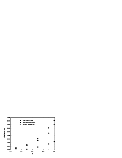
Figure 3: Relative errors of analytical harmonic amplitudes, Eqs.(12, 14, 15) with respect to numerically exact amplitudes.

Another important feature of the numerical FT of the solution of Eq.(17) is that the resolution of the mixed central peak in the middle between two fundamental second harmonics, Fig.2 (lower panel), essentially depends on the magnetic-field window used in FT, Fig.4.

Figure 4: Effect of the magnetic field window on the Fourier transform of magnetisation. Decreasing the window increases the width of FT harmonics obscuring the mixed harmonic.

Since the mixed amplitude is relatively small as $(B/2\pi B_{\perp})^{1/2}\ll 1$, the window affects its experimental resolution. We believe that a relatively small interval of the magnetic fields, used in FT, has prevented so far the single-band combination frequency to be seen in layered metals sin ; kar ; mac ; other . Importantly, since the characteristic field, $B_{\perp}\propto J_{0}(k_{F}d\tan(\Theta))/\cos(\Theta)$, is an oscillating function of the tilting angle $\Theta$, the combination amplitude also oscillates as the function of the angle, which could be instrumental in its experimental identification. We notice that the angle dependence of the second fundamental harmonics has been clearly observed in Sr₂RuO₄ other .

There is also mixing in the SdH quantum oscillations of transverse and longitudinal conductivities. For example the longitudinal conductivity is given by the Kubo formula kubo ,

$$\sigma=-\pi\hbar e^{2}\int dE{\partial f(E)\over{\partial E}}Tr[\delta(E-H)v_{\perp}\delta(E-H)v_{\perp})],$$ (18)

where $v_{\perp}=2td\sin(k_{\perp}d)/\hbar$ is the longitudinal component of the velocity operator, $H$ is the single-particle Hamiltonian including the impurity scattering, and $f(E)=1/[\exp(E-\mu)/k_{B}T+1]$ is the Fermi-Dirac distribution function. Averaging over random impurity distributions and approximating the scattering rate by a constant, $\Gamma$, one obtains the trace in Eq.(18) as $(v_{\perp}\Im[E-E_{n}(k_{\perp})-i\Gamma]^{-1})^{2}$ in the ladder approximation. Then applying Poisson’s summation, one can readily obtain a quantum correction, $\tilde{\sigma}$, to the classical conductivity (for detail see Refs. min ; gri ; alekab ), which is (at $T=0$)

$$\tilde{\sigma}\propto B\sum_{r=1}^{\infty}{(-R)^{r}\over{r}}J_{1}\left({4\pi rt\over{\hbar\omega_{c}}}\right)\cos\left(\frac{2\pi r\mu}{\hbar\omega_{c}}\right).$$ (19)

The asymptotic of the Bessel function, $J_{1}(x)\approx(2/\pi x)^{1/2}\cos(x+\pi/4)$, yields FTs of $\tilde{\sigma}$ very similar to those of magnetisation, Fig.2, with the combination harmonic in the canonical system. Generally the scattering rate depends on the magnetic field gri , so that its oscillations require more thorough analysis of the SdH effect, but mixing should be robust. Interestingly, some mixing of fundamental frequencies may occur even in grand-canonical multi- or single-band layered systems, if there is an inter-band or inter-extremal cross-section scattering by impurities.

In conclusion, we have found the combination frequency in the quantum magnetic oscillations of the single-band canonical layered Fermi liquid. The difference between quantum oscillations of the canonical and grand-canonical ensembles, is tiny, Fig.2, but not obscured by the MB effect, which is absent in the single-band case in contrast with the multi-band systems. We have also shown that the analytical (perturbative) FT amplitudes are numerically accurate even at zero temperature and in clean samples (i.e. for $R=1$) as they are in the multi-band analytical theory alebra3 ; comment . A wide magnetic-field window is essential for experimental resolution of the combination dHvA/SdH frequency.

We greatly appreciate valuable discussions with Iorwerth Thomas and support of this work by EPSRC (UK) (grant No. EP/D035589).

References

- (1) D. Schoenberg, Magnetic Oscillations in Metals (Cambridge University Press, Cambridge 1984).
- (2) J. Singleton, Rep. Prog. Phys. 63, 1111 (2000).
- (3) M. V. Kartsovnik, Chem. Rev. 104, 5737 (2004) and references therein.
- (4) A. P. Mackenzie, S. R. Julian, A. J. Diver, G. J. McMullan, M. P. Ray, G. G. Lonzarich, Y. Maeno, S. Nishizaki, and T. Fujita, Phys. Rev. Lett. 76, 3786 (1996).
- (5) A. S. Alexandrov and A. M. Bratkovsky, Phys. Rev. Lett. 76, 1308 (1996).
- (6) M. Nakano, J. Phys. Soc. Japan 66, 19 (1997).
- (7) A. S. Alexandrov and A. M. Bratkovsky, Phys. Lett. A 234, 53 (1997).
- (8) T. Champel, Phys. Rev. B 65, 153403 (2002); ibid 69, 167402 (2004).
- (9) A. S. Alexandrov and A. M. Bratkovsky, Phys. Rev. B 69, 167401 (2004).
- (10) K. Kishigi and Y. Hasegawa, Phys. Rev. B 65, 205405 (2002); ibid. 72, 045410 (2005).
- (11) A. S. Alexandrov and A. M. Bratkovsky, Phys. Rev. B 63, 033105 (2001).
- (12) A. M. Bratkovsky and A. S. Alexandrov, Phys. Rev. B 65, 035418 (2002).
- (13) J. Y. Fortin, E. Perez, and A. Audouard, Phys. Rev. B 71, 155101 (2005).
- (14) R. A. Shepherd, M. Elliott, W. G. Herrenden-Harker, M. Zervos, P. R. Morris, M. Beck, and M. Ilegems, Phys. Rev. B 60, R11277 (1999).
- (15) E. Ohmichi, Y. Maeno, and T. Ishiguro, J. Phys. Soc Japan 68, 24 (1999).
- (16) N. Harrison, J. Caulfield, J. Singleton, P. H. P. Reinders, F. Herlach, W. Hayes, M. Kurmoo, and P. J. Day, J. Phys. Condens. Matter 8, 5415 (1996); P. S. Sandhu, Ju H. Kim, and J. S. Brooks, Phys. Rev. B 56, 11566 (1997); J. H. Kim, S. Y. Han, and J. S. Brooks, Phys. Rev. B 60, 3213 (1999); S. Y. Han, J. S. Brooks, and J. H. Kim, Phys. Rev. Lett. 85, 1500 (2000); V. M. Gvozdikov and M. Taut, Phys. Rev. B 75, 155436 (2007); D. Vignolles, A. Audouard, V. N. Laukhin, J. Beard, E. Canadell, N. G. Spitsina, E. B. Yagubskii, Eur. Phys. J. B 55, 383 (2007).
- (17) Y. Kurihara, J. Phys. Soc. Japan 61, 975 (1989).
- (18) K. Yamaji, J. Phys. Soc. Japan 58, 1520 (1989).
- (19) R. Kubo, H. Hasegava, and N. Hashitsume, J. Phys. Soc. Japan 14, 56 (1959)).
- (20) T. Champel and V. P. Mineev, Phys. Rev. B 66, 195111 (2002); ibid 67, 089901 (2003).
- (21) P. D. Grigoriev, Phys. Rev. B 67, 144401 (2003).
- (22) A. S. Alexandrov and V. V. Kabanov, Phys. Rev. Lett. 95, 076601 (2005); ibid, 169902 (2005).