Mean field theory of spin glasses: statics and dynamics

Abstract

In these lectures I will review some theoretical results that have been obtained for spin glasses. I will concentrate my attention on the formulation of the mean field approach and on its numerical and experimental verifications. I will present the various hypothesis at the basis of the theory and I will discuss their mathematical and physical status.

1 Introduction

Spin glasses have been intensively studied in the last thirty years. They are very interesting for many reasons:

• Spin glasses are the simplest example of glassy systems. There is a highly non-trivial mean field approximation where one can study phenomena that have been discovered for the first time in this context, e.g. the existence of many equilibrium states and the ultrametricity relation among these states. In this framework it is possible to derive some of the main properties of a generic glassy systems, e.g. history dependent response [1, 2, 3]; this property, in the context of mean field approximation, is related to the existence of many equilibrium states .

• The study of spin glasses opens a very important window for studying off-equilibrium behavior. Aging [9] and the related violations of the equilibrium fluctuation dissipation relations emerge in a natural way and they can be studied in this simple setting [10, 11, 12, 13]. Many of the ideas developed in this context can be used in other physical fields like fragile glasses, colloids, granular materials, combinatorial optimization problems and for other complex systems [14].

• The theoretical concepts and the tools developed in the study of spin glasses are based on two logically equivalent, but very different, methods: the algebraic broken replica symmetry method and the probabilistic cavity approach [2, 3]. They have a wide domain of applications. Some of the properties that appear in the mean field approximation, like ultrametricity, are unexpected and counterintuitive.

• Spin glasses also provide a testing ground for a more mathematical inclined probabilistic approach: the rigorous proof of the correctness of the solution of the mean field model came out after twenty years of efforts where new ideas (e.g. stochastic stability [15, 16, 17]) and new variational principles [18, 19] were at the basis of a recent rigorous proof [20] of the correctness of the mean field approximation for in the case of the infinite range Sherrington-Kirkpatrick model [21].

In these lectures I will present a short review of some of the results that have been obtained using the probabilistic cavity approach. I will mostly discuss the mean field approximation for the infinite range Sherrington-Kirkpatrick. I will only mention en passant how to extend these results to finite connectivity model and to finite dimensional systems. The very interesting applications of these techniques to other problems coming from physics (e.g. glasses [22]) and other disciplines [14] will not be discussed.

2 General considerations

The simplest spin glass Hamiltonian is of the form:

$$H=\sum_{i,k=1,N}J_{i,k}\sigma_{i}\sigma_{k}\,,$$ (1)

where the $J$’s are quenched (i.e. time independent) random variables located on the links connecting two points of the lattice and the $\sigma$’s are Ising variables (i.e. they are equal to $\pm 1$). The total number of points is denoted with $N$ and it goes to infinity in the thermodynamic limit.

We can consider four models of increasing complexity:

• The SK model [21]: All $J$’s are random and different from zero, with a Gaussian or a bimodal distribution with variance $N^{-1/2}$. The coordination number ($z$) is $N-1$ and it goes to infinity with $N$. In this case a simple mean field theory is valid in the infinite $N$ limit [2, 3].

• The Bethe lattice model [23, 24, 25]: The spins live on a random lattice and only $Nz/2$ $J$’s are different from zero: they have variance $z^{-1/2}$. The average coordination number is finite (i.e. $z$). In this case a modified mean field theory is valid.

• The large range Edwards Anderson model [26]: The spins belong to a finite dimensional lattice of dimension $D$. Only nearest spins at a distance less than $R$ interact and the variance of the $J$’s is proportional to $1/R^{D/2}$. If $R$ is large, the corrections to mean field theory are small for thermodynamic quantities, although they may change the large distance behavior of the correlations functions and the nature of the phase transition, which may disappear.

• The Edwards Anderson model [27]: The spins belong to a finite dimensional lattice of dimensions $D$: Only nearest neighbor interactions are different from zero and their variance is $D^{-1/2}$. In this case finite corrections to mean field theory are present, that are certainly very large in one or two dimensions, where no transition is expected. The Edwards Anderson model corresponds to the limit $R=1$ of the the large range Edwards Anderson model; both models are expected to belong to the same universality class. The large range model Edwards Anderson provides a systematic way to interpolate between the mean field results and the short range model .

As far as the free energy is concerned, one can prove the following rigorous results:

$$\lim_{z\to\infty}\mbox{Bethe}(z)=\mbox{SK}\ ,$$ (2)

$$\lim_{D\to\infty}\mbox{Edwards Anderson}(D)=\mbox{SK}\ ,$$

$$\lim_{R\to\infty}\mbox{finite range EA}(R)=\mbox{SK}\ .$$

The Sherrington Kirkpatrick model is thus a good starting point for studying also the finite dimensional case with short range interaction, that is the most realistic and difficult case. This starting point becomes worse and worse when the dimension decreases, e.g. it is not any more useful in the limiting case where $D=1$.

3 Mean field theory

3.1 General considerations

Let us start again with the Hamiltonian in eq. (1) and let us proceed in the most naive way. Further refinements will be added later.

We consider the local magnetizations $m_{i}=\langle\sigma_{i}\rangle$ and we write the simplest possible form of the free energy as function of the magnetization. Using the standard arguments, that can be found in books [5], we get:

$$F[m]=\sum_{i,k=1,N}J_{i,k}m_{i}m_{k}-T\sum_{i}S(m_{i})\ ,$$ (3)

where $S(m)$ is the usual binary entropy:

$$-S(m)=\frac{1}{2}\left(\frac{1+m}{2}\log\left(\frac{1+m}{2}\right)+\frac{1-m}{2}\log\left(\frac{1-m}{2}\right)\right)\ .$$ (4)

If we look to the minimum of the free energy, we get the following equations (that are valid at any stationary point of the free energy):

$$m_{i}=\mbox{th}(h^{eff}_{i}),\ \ \ \ \ \ h^{eff}_{i}=\sum_{k}J_{i,k}\sigma_{k}\ .$$ (5)

This is well known and fifty years ago we could have stopped here. However now we understand that mean field approximation involves uncontrolled approximations and therefore we need to work in a more controlled framework.

In a more modern approach one consider a model and one tries to write down an expression for the free energy that is exact for that particular model. In this way one is sure that the range of validity of the formulae one is writing is not void (and what is more important, if no technical mistakes have been done, there could be no contradictions). As far as the exact model is often obtained as limit of a more realistic model when some parameter goes to infinity, it is possible to estimate the corrections to these asymptotic results.

A very interesting case, where usually mean field exact formula are valid, happens when the coordination number (i.e. the number of spins that are connected to a given spin) goes to infinity. Let us consider the following construction. We assume that for a given $i$, $J_{i,k}$ is different from zero only for $z$ different values of $k$ (for simplicity let us also assume that the $J$’s take only the values $\pm 1$ with equal probability).

We are interested to study the limit where $z$ goes to infinity. One can immediately see that in the random case a finite result is obtained (at least in the high temperature phase) only if $J$ goes to zero as $z^{-1/2}$ (a similar result can be obtained also in the low temperature phase). This result is in variance with the ferromagnetic case where the $J$’s are all positive and they should go zero as $z$ in order to have a finite result in the low temperature phase. Indeed a good thermodynamic scaling is present when $h^{eff}$ is of O(1). In the ferromagnetic case the $z$ terms in the expression for $h^{eff}$ add coherently and therefore each of them must be of order $z^{-1}$; on the contrary in the spin glass case, if they are uncorrelated (this is true in a first approximation), $h^{eff}$ is the sum of $z$ random terms and the result is of O(1) only if each term is of order $z^{-1/2}$.

If one makes a more careful computation and we look to the corrections to the mean field expression that survive in this limit, one obtains:

$$F_{TAP}[m]=$$ (6)

$$\sum_{i,k=1,N}\left(\frac{1}{2}J_{i,k}m_{i}m_{k}-\frac{1}{4}\beta J_{i,k}^{2}(1-m_{i}^{2})(1-m_{k}^{2})\right)-T\sum_{i}S(m_{i})\ ,$$

where $\beta=1/T$ (we put the Boltzmann-Drude constant $\alpha$ to the value 3/2).

This free energy has an extra term with respect to the previous free energy eq. (5) and is called the TAP free energy [28], because it firstly appeared in a preprint signed by Thouless, Anderson, Lieb and Palmer . The extra term can be omitted in the ferromagnetic case, because it gives a vanishing contribution.

We must add a word of caution: the TAP free energy has not been derived from a variational equation: the magnetization should satisfy the the stationary equation:

$${\partial F\over\partial m_{i}}=0\ ,$$ (7)

but there is no warranty that the correct value of the magnetization is the absolute minimum of the free energy. Indeed in many cases the paramagnetic solution (i.e. $m_{i}=0$) is the absolute minimum at all temperatures, giving a value of the free energy density that would be equal to $-\frac{1}{4}\beta$. The corresponding internal energy would be equal to $-\frac{1}{2}\beta$: it would give an result divergent at $T=0$, that in most of the cases would be unphysical.

Let us be more specific (although these consideration are quite generic) and let us consider the case of the Sherrington Kirkpatrick model, where all spins are connect and $z=N-1$.

Here one could be more precise and compute the corrections to the TAP free energy: an explicit computation shows that these corrections are not defined in some regions of the magnetization space [1, 29]. When the corrections are not defined, the TAP free energy does not make sense. In this way (after a detailed computation) one arrives the conclusion that one must stay in the region where the following condition is satisfied:

$$\beta^{2}\mbox{Av}\left((1-m_{i}^{2})^{2}\right)\leq 1\ ,$$ (8)

where Av stands for the average over all the points $i$ of the sample. When the previous relation is not valid, one finds that the correlations function, that were assumed to be negligible, are divergent [2] and the whole computation fails. The correct recipe is to find the absolute minimum of the TAP free energy only in this region [1]. Of course the paramagnetic solution is excluded as soon as $T<1$.

Let us as look to the precise expression of the TAP stationarity equations: they are

$$m_{i}=\mbox{th}(\beta h^{eff}_{i})\ ,\ \ \ \ \ h^{eff}_{i}=\sum_{k}\left(J_{i,k}m_{k}-\beta m_{i}J_{i,k}^{2}(1-m_{k}^{2})\right)\ .$$ (9)

For large $N$ these equations can be simplified to

$$h_{i}=\sum_{k}\left(J_{i,k}m_{k}-\beta m_{i}(1-q_{EA})\right)\ ,$$ (10)

where

$$q_{EA}=\mbox{Av}(m_{i}^{2})\ .$$ (11)

Apparently the TAP equations are more complex that the naive ones (5); in reality their analysis is simpler. Indeed, using perturbation expansion with respect to the term $J_{i,k}$ that are of order $O(N^{1/2})$, we can rewrite the effective field as

$$h^{eff}_{i}=\sum_{k}J_{i,k}m^{c}_{k}\ ,$$ (12)

where the cavity magnetizations $m^{c}_{k}$ are the values of the magnetizations at the site $k$ in a system with $N-1$ spins, where the spin at $i$ has been removed [2] (the correct notation would be $m^{c}_{k;i}$ in order to recall the dependence of the cavity magnetization on the spin that has removed, but we suppress the second label $i$ when no ambiguities are present). The previous equations are also called Bethe’s equations because they were the starting point of the approximation Bethe in his study of the two dimensional Ising model.

The crucial step is based on the following relation:

$$m_{k}=m^{c}_{k}+\beta m_{i}J_{i,k}(1-(m^{c}_{k;i})^{2})\ .$$ (13)

This relation can be proved by using the fact that the local susceptibility $\partial m_{i}/\partial h_{i}$ is given by $\beta(1-m_{i}^{2})$ in the mean field approximation. Although the difference between $m(k)$ and $m^{c}_{k}$ is small, i.e. O($N^{-1/2}$), one obtains that the final effect on $h_{eff}$ is of O(1).

The validity of eq. (12) is rather fortunate, because in this formula $J_{i,k}$ and $m^{c}_{k}$ are uncorrelated. Therefore the central limit theorem implies that, when one changes the $J_{i,k}$, the quantity $h^{eff}_{i}$ has a Gaussian distribution with variance $q_{EA}$. Therefore the probability distribution of $h^{eff}$ is given by

$$P(h)dh=(2\pi)^{-1/2}\exp(-q^{2}/2)dh\equiv d\mu_{q}(h)$$ (14)

However this result is valid only under the hypothesis that there is a one to one correspondence of the solutions of the TAP equation at $N$ and at $N-1$, a situation that would be extremely natural if the number of solutions of the TAP equations would be a fixed number (e..g 3, as happens in the ferromagnetic case at low temperature). As we shall see, this may be not the case and this difference brings in all the difficulties and the interesting features of the models.

3.2 The cavity method: the naive approach

Given the fact that all the points are equivalent, it is natural to impose the condition that the statistical properties of the spin at $i$, when the $J_{i,k}$ change, are $i$ independent. For a large system this statistical properties coincide with those obtained by looking to the properties of the other $N-1$ spins of the system. This condition leads to the cavity method, where one compare the average properties of the spins in similar systems with slightly different size.

The cavity method is a direct approach that in principle can be used to derive in an probabilistic way all the results that have been obtained with the replica method . The replica approach is sometimes more compact and powerful, but it is less easy to justify, because the working hypothesis that are usually done cannot be always translated in a transparent way in physical terms .

The idea at the basis of the cavity method is simple: we consider a system with $N$ spins ($i=1,N$) and we construct a new system with $N+1$ spins by adding an extra spin ($\sigma_{0}$). We impose the consistency condition that the average properties of the new spin (the average being done with respect to $J_{0,i}$) are the same of that of the old spins [2, 24].

In this way, if we assume that there is only one non-trivial solution to the TAP equations , we get that for that particular solution

$$\overline{m_{0}^{2}}=\mbox{Av}(m_{i}^{2})\ ,$$ (15)

where the bar denotes the average over all the $J_{0,i}$.

The Hamiltonian of the new spin is:

$$\sigma_{0}\sum_{i=1,N}J_{0,i}\sigma_{i}\ .$$ (16)

If we suppose that the spins $\sigma_{i}$ have vanishing correlations and we exploit the fact that each individual term of the Hamiltonian is small, we find that

$$m_{0}\equiv\langle\sigma_{0}\rangle=\tanh(\beta h^{eff})\ .$$ (17)

$$h^{eff}=\sum_{i=1,N}J_{0,i}m^{c}_{i}\ ,$$

where $m^{c}_{i}$ (for $i\neq 0$) denotes the magnetization of the spin $\sigma_{i}$ before we add the spin 0. In this way we have rederived the TAP equations for the magnetization in a direct way, under the crucial hypothesis of absence of long range correlation among the spins (a result that should be valid if we consider the expectation values taken inside one equilibrium state). It should be clear why the whose approach does not make sense when the condition eq. (8) is not satisfied.

We have already seen that when the variables $J_{0,i}$ are random, the central limit theorem implies that $h$ is a Gaussian random variable with variance

$$\overline{h^{2}}=q_{EA}\equiv{\sum_{i=1,N}(m^{c}_{i})^{2}\over N}\ ,$$ (18)

and the distribution probability of $h$ is given by eq. (14). The same result would be true also when the variables $m^{c}_{i}$ are random.

If we impose the condition that the average magnetization squared of the new point is equal to average over the old points, we arrive to the consistency equation:

$$q_{EA}=\overline{m_{0}^{2}}=\int d\mu_{q_{EA}}(h)\tanh^{2}(\beta h)\ ,$$ (19)

where $d\mu_{q_{EA}}(h)$ denotes a normalized Gaussian distribution with zero average and variance $q_{EA}$. It is easy to check [2] that the $h$-dependent increase in the total free energy of the system (when we go from $N$ to $N+1$) is

$$\beta\Delta F(h)\equiv-\ln(\cosh(\beta h))\ .$$ (20)

It is appropriate to add a comment. The computation we have presented relates the magnetization a spin of the systems with $N+1$ spins to the magnetizations of the system with $N$ spins: they are not a closed set of equations for a given system. However we can also write the expression of magnetization at the new site as function of the magnetizations of the system with $N+1$ spins, by computing the variation of the magnetizations in a perturbative way. Let us denote by $m$ the magnetization of the old system ($N$ spins) and by $m^{\prime}$ the magnetization of the new system ($N+1$ spins). Perturbation theory tell us that

$$m^{\prime}_{i}\approx m_{i}+J_{0,i}m^{\prime}_{0}{\partial m_{i}\over h_{i}}=m_{i}+J_{0,i}m^{\prime}_{0}\beta(1-(m^{\prime}_{i})^{2})\ .$$ (21)

It is not surprising that using the previous formula we get again the TAP equations [28, 2]:

$$m^{\prime}_{0}=\tanh(\beta h)\,$$

$$h=\sum_{i=1,N}J_{0,i}m_{i}\approx\sum_{i=1,N}J_{0,i}m^{\prime}_{i}-m^{\prime}_{0}\sum_{i}J_{0,i}^{2}\beta(1-m^{\prime}_{i})\,$$ (22)

$$\approx\sum_{i=1,N}J_{0,i}m^{\prime}_{i}-m^{\prime}_{0}\beta(1-q_{EA})\,$$

where $(N+1)q_{EA})=\sum_{i=0,N}m^{\prime}_{i}$ (we have used the relation $\overline{J_{0,i}^{2}}=N^{-1}$).

A detailed computation show that the free energy corresponding to a solution of the TAP equations is given by the TAP free energy. The computation of the total free energy is slightly tricky. Indeed we must take care than if we just add one spin the coordination number $z$ change and we have to renormalize the $J$’s. This gives an extra term that should be taken into account.

The explicit computation of the free energy could be avoided by computing the internal energy density and verifying a a posteriori the guessed form of the free energy is correctly related to the internal energy. Here we can use a general argument: when the $J$’s are Gaussianly distributed the internal energy density $e$ is given

$$e=\frac{1}{2}\overline{\sum_{i}J_{0,i}\langle\sigma_{0}\sigma_{i}\rangle}=\frac{1}{2N}\overline{\sum_{i}\frac{\partial}{J_{0,i}}\langle\sigma_{0}\sigma_{i}\rangle}=$$ (23)

$$\beta\frac{1}{2N}\overline{\sum_{i}(\langle(\sigma_{0}\sigma_{i})^{2}\rangle-\langle\sigma_{0}\sigma_{i}\rangle^{2})}=\frac{1}{2}\beta(1-q^{2})\ .$$

In the first step we have integrated by part with respect to the Gaussian distribution of the $J$, in the last step se have used the assumption that connect correlation are small and therefore

$$\langle\sigma_{0}\sigma_{i}\rangle^{2}\approx(m_{0}m_{i})^{2}\ .$$ (24)

In both ways one obtain the expression for the TAP free energy, where the only parameter free is $q\equiv q_{EA}$; we can call this quantity $f(q)$; its explicit expression is

$$\beta f(q)=-\frac{1}{4}\beta^{2}(1-q^{2})+\int d\mu_{q}(h)\ln\left(\cosh(\beta h)\right)$$ (25)

The value of $q$ can be computed in two mathematical equivalent ways:

• We use the equation (19) to find a non-linear equation for $q$.

• We find the stationary point of the free energy respect to $q$ by solving the equation $\partial f/\partial q=0$.

An integration by part is the needed step to prove the equivalence of the two computations.

An explicit computation shows that the non-trivial stationary point (i.e $q\neq 0$), that should be relevant at $T<1$, is no not a minimum of the free energy, as it should be a maximum for reasons that would be clear later. In this way one finds the form of the function $q(T)$. which turns out to be rather smooth:

• $q(T)$ is zero for $T>1$.

• $q(T)$ it is proportional to $1-T$ for $T$ slightly below 1.

• $q(T)$ behave as $1-AT$, with positive $A$ when $T$ goes to zero.

When this solution was written down [21], it was clear that something was wrong. The total entropy was negative at low temperature. This was particular weird, because in usual mean field models the entropy is just the average over the sites of the local entropy that is naturally positive. The villain is the extra term that we have added to the naive free energy in order to get the TAP free energy: indeed one finds that the entropy density is given by

$$S=\mbox{Av}(S(m_{i}))-\frac{(1-q)^{2}}{4T^{2}}\ .$$ (26)

The average of the local term goes like $T$ at low temperatures, while the extra term goes to $-A^{2}/4$, i.e. -0.17. It is important to note that the extra term is needed to obtain that for $T>1$, $e=-\beta/2$, a results that can be easily checked by constructing the high temperature expansion.

On the contrary numerical simulations [21] showed a non-negative entropy (the opposite would be an extraordinary and unexpected event) very similar to the analytic computation for $T>0.4$ and going to zero at $T^{2}$ (the analytic result was changing sign around $T=.0.3$).

Also the value of the internal energy was wrong: the analytic computation gave $e=-0.798$ while the numerical computations gave $e=-0.765\pm 0.01$ (now numerical simulations give $e=-0.7633\pm 0.0001)$.

It is clear that we are stacked, the only way out is to leave out the hypothesis of the existence of only one solution of the TAP equations (or equivalently of only one equilibrium state) and to introduce this new ingredient in the approach. This will be done in the next section.

4 Many equilibrium states

4.1 The definition of equilibrium states

The origin of the problem firstly became clear when De Almeida and Thouless noticed that in the whole region $T<1$, the inequality (8) was violated:

$$\beta^{2}\mbox{Av}\left((1-m_{i}^{2})^{2}\right)=1+B_{0}(1-T)^{2}\,,$$ (27)

with $B_{0}$ positive.

The problem became sharper when it was rigorously proved that the wrong naive result was a necessary consequence of the existence of a only one equilibrium state, i.e. of the assumption that connected correlations functions are zero (in an infinitesimal magnetic field) and therefore

$$\langle\sigma_{i}\sigma_{k}\rangle\approx\langle\sigma_{i}\rangle\langle\sigma_{k}\rangle\ .$$ (28)

In order to develop a new formalism that overcomes the pitfalls of the naive replica approach, it is necessary to discuss the physical meaning of these results and to consider the situation where many states are present. The first step consists in introducing the concept of pure states in a finite volume [2, 6]. This concept is crystal clear from a physical point of view, however it is difficult to state it in a rigorous way. We need to work at finite, but large volumes, because the infinite volume limit for local observables is somewhat tricky and we have a chaotic dependence on the size [4, 6].

At this end we consider a system with a total of $N$ spins. We partition the equilibrium configuration space into regions, labeled by $\alpha$, and each region must carry a finite weight. We define averages restricted to these regions [7, 8, 6]: these regions will correspond to our finite volume pure states or phases. It is clear that in order to produce something useful we have to impose sensible constraints on the form of these partitions. We require that the restricted averages on these regions of phase space are such that connected correlation functions are small when the points are different in an infinite range model. This condition is equivalent to the statement that the fluctuation of intensive quantities vanishes in the infinite volume limit inside a given phase.

The phase decomposition depends on the temperature. In a ferromagnet at low temperature two regions are defined by considering the sign of the total magnetization. One region includes configurations with a positive total magnetization, the second selects negative total magnetization. There are ambiguities for those configurations that have exactly zero total magnetization, but the probability that these configurations are present at equilibrium is exponentially small at low temperature.

In order to present an interpretation of the results we assume that such decomposition exists also each instance of our problem. Therefore the finite volume Boltzmann-Gibbs measure can be decomposed in a sum of such finite volume pure states and inside each state the connect correlations are small. The states of the system are labeled by $\alpha$: we can write

$$\langle\ \cdot\ \rangle=\sum_{\alpha}w_{\alpha}\langle\ \cdot\ \rangle_{\alpha}\ ,$$ (29)

with the normalization condition

$$\sum_{\alpha}w_{\alpha}=1-\epsilon\ ,$$ (30)

where $\epsilon\to 0$ when $N\to\infty$.

The function $P_{J}(q)$ for a particular sample is given by

$$P_{J}(q)=\sum_{\alpha,\beta}w_{\alpha}w_{\beta}\delta(q_{\alpha,\beta}-q)\ ,$$ (31)

where $q_{\alpha,\gamma}$ is the overlap among two generic configurations in the states $\alpha$ and $\gamma$:

$$q_{\alpha,\gamma}={\sum_{1=1,N}m_{\alpha}(i)m_{\gamma}(i)\over N}\ ,$$ (32)

and $m_{\alpha}(i)$ and $m_{\gamma}(i)$ are respectively the magnetizations within the state $\alpha$ and $\gamma$.

For example, if we consider two copies (i.e. $\sigma$ and $\tau$) of the same system, we have;

$$q[\sigma,\tau]={\sum_{1=1,N}\sigma(i)\tau(i)\over N}$$ (33)

and

$$\langle g(q[\sigma,\tau])\rangle_{J}=\int g(q)P_{J}(q)dq\ ,$$ (34)

where $g(q)$ is a generic function of $q$.

Given two spin configurations ($\sigma$ and $\tau$) we can introduce the natural concept of distance by

$$d^{2}(\sigma,\tau)\equiv\frac{1}{2N}\sum_{i=1}^{N}(\sigma_{i}-\tau_{i})^{2}\ ,$$ (35)

that belongs to the interval [0 - 2], and is zero only if the two configurations are equal (it is one if they are uncorrelated). In the thermodynamical limit, i.e. for $N\to\infty$, the distance of two configurations is zero if the number of different spins remains finite. The percentage of different $\sigma$’s, not the absolute number, is relevant in this definition of the distance. It is also important to notice that at a given temperature $\beta^{-1}$, when $N$ goes to infinity, the number of configurations inside a state is extremely large: it is proportional to $\exp(N{S}(\beta))$, where ${S}(\beta)$ is the entropy density of the system).

In a similar way we can introduce the distance between two states defined as the distance among two generic configurations of the states:

$$d^{2}_{\alpha,\gamma}=1-q_{\alpha,\gamma}\ .$$ (36)

In the case where the self-overlap

$$q_{\alpha,\alpha}={\sum_{1=1,N}m_{\alpha}(i)^{2}\over N}\ ,$$ (37)

does not depend on $\alpha$ and it is denoted by $q_{EA}$, we have that the distance of a state with itself is not zero:

$$d^{2}_{\alpha,\alpha}=1-q_{EA}\ .$$ (38)

We expect that finite volume pure states will enjoy the following properties that hopefully characterizes the finite volume pure states [6, 7]:

• When $N$ is large each state includes an exponentially large number of configurations .

• The distance of two different generic configurations $C_{\alpha}$ and $C_{\gamma}$ (the first belonging to state $\alpha$ and the second to state $\gamma$) does not depend on the $C_{\alpha}$ and $C_{\gamma}$, but only on $\alpha$ and $\beta$. The distance $d_{\alpha,\gamma}$ among the states $\alpha$ and $\gamma$, is the distance among two generic configurations in these two states. The reader has already noticed that with this definition the distance of a state with itself is not zero. If we want, we can define an alternative distance:

  $$D_{\alpha,\gamma}\equiv d_{\alpha,\gamma}-\frac{1}{2}\left(d_{\alpha,\alpha}+d_{\gamma,\gamma}\right)\ ,$$ (39)

  in such a way that the distance of a state with itself is zero ($D_{\alpha,\alpha}=0$).

• The distance between two configurations belonging to the same state $\alpha$ is strictly smaller than the distance between one configuration belonging to state $\alpha$ and a second configuration belonging to a different state $\gamma$. This last property can be written as

  $$d_{\alpha,\alpha}<d_{\alpha,\gamma}\ \mbox{if}\ \alpha\neq\gamma\ .$$ (40)

  This property forbids to have different states such that $D_{\alpha,\gamma}=0$, and it is crucial in avoiding the possibility of doing a too fine classification .

• The classification into states is the finest one that satisfies the three former properties.

The first three conditions forbid a too fine classification, while the last condition forbids a too coarse classification.

For a given class of systems the classification into states depends on the temperature of the system. In some case it can be rigorously proven that the classification into states is possible and unique [30, 31] (in these cases all the procedures we will discuss lead to the same result). In usual situations in Statistical Mechanics the classification in phases is not very rich. For usual materials, in the generic case, there is only one state. In slightly more interesting cases there may be two states. For example, if we consider the configurations of a large number of water molecules at zero degrees, we can classify them as water or ice: here there are two states. In slightly more complex cases, if we tune carefully a few external parameters like the pressure or the magnetic field, we may have coexistence of three or more phases (a tricritical or multicritical point).

In all these cases the classification is simple and the number of states is small. On the contrary in the mean field approach to glassy systems the number of states is very large (it goes to infinity with $N$), and a very interesting nested classification of states is possible. We note “en passant” that this behavior implies that the Gibbs rule is not valid for spin glasses.

We have already seen the only way out from the inconsistent result of the naive approach is to assume the existence of many equilibrium states. A more precise analysis will show that we need not only a few equilibrium states but an infinite number and which are the properties of these states.

4.2 The description of a many states system

The next step consists in describing a system with many equilibrium state and to find out which is the most appropriate way to code the relevant information,

Let us assume that a system has many states. In equation

$$\langle\ \cdot\ \rangle=\sum_{\alpha}w_{\alpha}\langle\ \cdot\ \rangle_{\alpha}\ ,$$ (41)

there is a large number of $w$’s that are non-zero.

How are we are supposed to describe such a system? First of all we should give the list of the $w_{\alpha}$. In practice it is more convenient to introduce the free energy of a state $F_{\alpha}$ defined by

$$w_{\alpha}\propto\exp(-\beta F_{\alpha})\ ,$$ (42)

where the proportionality constant is fixed by the condition of normalization of the $w$’s, i.e. eq. (30). Of course the free energies are fixed modulo an overall addictive constant,

The second problem it to describe the states themselves. In this context we are particularly interested in describing the relations among the different states. At this end we can introduce different kinds of overlaps:

• The spin overlap, which we have already seen, i.e.

  $$q_{\alpha,\gamma}=N^{-1}\sum_{i}\langle\sigma_{i}\rangle_{\alpha}\langle\sigma_{i}\rangle_{\gamma}\ .$$ (43)

• The link (or energy) overlap, which is defined as:

  $$q^{L}_{\alpha,\gamma}=N^{-1}\sum_{i,k}J_{i,k}\langle\sigma_{i}\sigma_{k}\rangle_{\alpha}J_{i,k}\langle\sigma_{i}\sigma_{k}\rangle_{\gamma}\ .$$ (44)

• We could introduce also more fancy overlaps like

  $$q^{(l)}_{\alpha,\gamma}=N^{-1}\sum_{i,k}J^{(l)}_{i,k}\langle\sigma_{i}\sigma_{k}\rangle_{\alpha}J^{(l)}_{i,k}\langle\sigma_{i}\sigma_{k}\rangle_{\gamma}\ ,$$ (45)

  where $J^{(l)}$ denotes the $l$-th power of the matrix $J$.

• More generally, in the same way as the distances we can introduce overlaps that depend on the local expectation value of an operator $O(i)$

  $$q^{(O)}_{\alpha,\gamma}=N^{-1}\sum_{i}\langle O(i)\rangle_{\alpha}\langle O(i)\rangle_{\gamma}\ ,$$ (46)

In principle the description of the system should be given by the list of all $F_{\alpha}$ and by the list of all possible overlaps a between all the pairs $\alpha,\gamma$. However it may happens, as it can be argued to happen in the SK model, that all overlap are function of the same overlap $q$. For example in the SK model we have

$$q^{L}=q^{2}\ .$$ (47)

More complex formulae holds for the other overlaps.

In the case in short range model we may expect that

$$q^{L}=l(q^{2})\,$$ (48)

where $l(q)$ is a model (and temperature) dependent function [32, 33]

If this reductio ad unum happens, we say that we have overlap equivalence and this is a property that has far reaching consequences. The simplest way to state this properties is the following. We consider a system composed by two replicas ($\sigma$ and $\tau$) and let us denote by $\langle\cdot\rangle_{q}$ the usual expectation Boltzmann-Gibbs expectation value with the constraint that

$$q[\sigma,\tau]=q\ .$$ (49)

Overlap equivalence states that in this restricted ensemble of the connected correlation functions of the overlap (and of the generalized overlaps) are negligible in the infinite range case (they would decay with the distance in a short range model).

There is no a priori compulsory need for assuming overlap equivalence; however it is by far the simplest situation and before considering other more complex cases it is better to explore this simple scenario, that it is likely to be valid at least in the SK model.

If overlap equivalence holds, in order to have a macroscopic description of the system, we must know only the list of all $F_{\alpha}$ and the list of al $q_{\alpha,\gamma}$. As we have already mentioned, we can also assume that for large $N$ $q_{\alpha,\alpha}$ does not depend on $\alpha$ and it is equal to $q_{EA}$ (this property is a consequence that the states cannot be distinguished one form the other using intrinsic properties). At the end the high level description of the system is given by [7, 19]:

$${\cal D}=\{q_{EA},\{F_{\alpha}\},\{q_{\alpha,\gamma}\}\}\ ,$$ (50)

where the indices $\alpha$ and $\gamma$ goes from 1 to $\Omega(N)$, where $\Omega(N)$ is a function that goes to infinity with $N$. The precise way in which $\Omega(N)$ increases with $N$ is irrelevant because all high free energy states give a very small contribution to statistical sums.

In a random system the descriptor $\cal D$ is likely to depend on the system , therefore we cannot hope to compute it analytically. The only thing that we can do is to compute the probability distribution of the descriptor ${\cal P}(D)$. Some times one refer to this task as high level statistical mechanics [7] because one has to compute the probability distribution of the states of the system an not of the configurations, as it is done in the old bona fide statistical mechanics (as it was done in the low level statistical mechanics).

4.3 A variational principle

Low level and high level statistical mechanics are clearly intertwined, as it can be see from the following considerations, where one arrives to computing the free energy density of the SK model using a variational principle.

Here we sketch only the main argument (the reader should read the original papers [18, 19]). Here for simplicity we neglect the terms coming for the necessity of renormalize the $J$ when we change $N$; these terms can be added at the price of making the formalism a little heavier.

Let us consider an SK system with $N$ particles with a descriptor ${\cal D}_{N}$. If we add a a new site we obtain a descriptor ${\cal D}_{N+1}$ where the overlaps do not change and the new free energies are given by

$$F_{\alpha}(N+1)=F_{\alpha}(N)+\Delta F_{\alpha},\ \ \ \ \ \beta\Delta F_{\alpha}={-\ln(\cosh(\beta h_{\alpha}))}$$ (51)

where

$$h_{\alpha}=\sum_{i}J_{0,i}m_{\alpha}(i)\ .$$ (52)

Also in the case where the $h_{\alpha}$ are Gaussian random uncorrelated, the fact that the new free energy depends on $h_{\alpha}$ implies that at fixed value of the free energy $F_{\alpha}(N+1)$ the corresponding value of the old free energy $F_{\alpha}(N)$ is correlated with $h_{\alpha}$. It is a problem of conditioned probability. If we look at the distribution of $h_{\alpha}$, conditioned at the value of the old free energy $F_{\alpha}(N)$, we find a Gaussian distribution, but if we look to the same quantity, conditioned at the value of $F_{\alpha}(N+1)$, the distribution is no more Gaussian. Therefore if we extract a state with a probability proportional to $w_{\alpha}\propto\exp(-\beta F_{\alpha}(N+1))$ the distribution of $h_{\alpha}$ will be not Gaussian.

Now it is clear that the $h_{\alpha}$ (conditioned to the old values of the free energy) are random Gaussian correlated variables because

$$\overline{h_{\alpha}h_{\gamma}}=q_{\alpha,\gamma}\ .$$ (53)

This correlation induces correlations among the $\Delta F_{\alpha}$.

Let us suppose for simplicity that we have succeeded in finding a choice of ${\cal P}({\cal D})$ that is self-reproducing, i.e. a probability distribution such that

$${\cal P}_{N+1}({\cal D})={\cal P}_{N}({\cal D})\ .$$ (54)

We have neglect an overall shift $\Delta F({\cal P})$ of the free energies, that obviously depend on ${\cal P}$. The self-reproducing property is non-trivial as we shall see later. Notice than in going from $N$ to $N+1$ the $q$’s do not change, so the crucial point are the correlations among the $q$’s and the $F$’s that may change going form $N$ to $N+1$.

A very interesting variational principle [19] tell us that the true free energy density $f$ is given by

$$f=\max_{{\cal P}}\Delta F({\cal P})\ ,$$ (55)

which automatically implies that

$$f\geq\Delta F({\cal P})\ \ \ \forall{\cal P}\ .$$ (56)

The reader should notice that there are no typos in the previous formulae. The free energy is the maximum, and not the minimum, with respect to all possible probabilities of the descriptor. It is difficult to explain why these inequalities are reversed with respect to the usual ones.

We could mumble that in random system we have to do the average over the logarithm of the free energy and the logarithm has the opposite convexity of the exponential. This change of sign is very natural also using the replica approach, but it is not trivial to give a compulsory physical explanation. The only suggestion we can give is follow the details of the proof.

The mathematical proof is not complex, there is a simpler form of this inequality that has been obtained by an interpolating procedure by Guerra [18] that is really beautiful and quite simple (it involves only integration by part and the notion that a square in non-negative).

We must add a remark: although the theorem tells us that the correct value of the free energy is obtained for a precise choice of the probability ${\cal P}^{*}({\cal D})$ that maximize eq. (55), there is no warranty that the actual form of the probability of the descriptors is given by ${\cal P}^{*}({\cal D})$. Indeed the theorem itself does not imply that the concept of descriptor is mathematical sound; all the heuristic interpretations of the descriptor and of the meaning of the theorem is done at risk of the physical reader.

While the lower bound is easy to use, for particular cases it coincides with Guerra’s one [18], in this formalism it is particularly difficult to find a ${\cal P}({\cal D})$ such that it is the actual maximum. The only thing that we are able to do is to prove by other means [20] which is the value of $f$ and to find out a ${\cal P}^{*}({\cal D})$ that it saturate the bounds [2]. It uniqueness (if restricted to the class of functions that satisfy eq. (54)), is far from being established. It is clear that we miss some crucial ingredient in order to arrive to a fully satisfactory situation.

5 The explicit solution of the Sherrington Kirkpatrick model

5.1 Stochastic Stability

The property of stochastic stability was introduced in a different context [15, 16, 17], however it is interesting to discuss them in this perspective. Stochastic stability stability is crucial because it strongly constrains the space of all possible descriptors and it is the hidden responsible of most of the unexpected cancellations or simplifications that are present in the computation of the explicit solution of the Sherrington Kirkpatrick model.

Let us sketch the definition of stochastic stability in this framework. Let us consider a distribution ${\cal P}({\cal D})$ and let us consider a new distribution ${\cal P}^{\prime}({\cal D})$ where

$$F^{\prime}_{\alpha}=F_{\alpha}+r_{\alpha}\ .$$ (57)

Here the $r$’s are random variables such that the correlation among $r_{\alpha}$ and $r_{\gamma}$ is a function of only $q_{\alpha,\gamma}$. We say that the distribution is stochastically stable iff the new distribution is equal to the previous one, after averaging over the $r$’s, apart from an overall shift or the $F$’s, i.e. iff

$${\cal P}({\cal D})={\cal P}^{\prime}({\cal D})\ .$$ (58)

It is evident that, if a distribution is stochastically stable, it is automatically self-reproducing because the the shifts in free energy can be considered random correlated variables. This strongly suggest to consider only stochastic stable $cP({\cal D})$. Moreover general arguments, that where at the origin of the first version of stochastic stability [15, 16, 17] imply that ${\cal P}({\cal D})$ should be stochastically stable.

More precisely the original version of stochastic stability implies the existence of a large set of sum rules, which can be derived in this context if we assume that the equation (58) is valid. These sum rules give relations among the joint average of the overlap of more real replicas (i.e. a finite number of copies of the system in the same realization of the quenched disorder). One can show [34] that under very general assumptions of continuity that also valid in finite dimensional models for the appropriate quantities.

These relations connects the expectation values of products of various functions $P_{J}(q)$ to the expectation value of the function $P_{J}(q)$ itself.

An example of these relations is the following

$$P(q)=\overline{P_{J}(q)}\ ,$$

$$P(q_{1,2},q_{3,4})\equiv\overline{P_{J}(q_{1,2})P_{J}(q_{3,4})}=$$ (59)

$$\frac{2}{3}P(q_{1,2})P(q_{3,4})+\frac{1}{3}P(q_{1,2})\delta(q_{1,2}-q_{3,4})\ .$$

where we have denoted by an bar the average over the $J$’s.

This relation is difficult to test numerically, as far as in finite volume systems we do not have exact delta functions, therefore very often one test simplified versions of these equations. For example let us consider four replicas of the system (all with the same Hamiltonian) and we denote by

$$E(\ldots)\equiv\overline{\langle\ldots\rangle}$$ (60)

the global average, taken both over the thermal noise and over the quenched disorder. The previous equation implies that

$$E(q_{1,2}^{2}q_{3,4}^{2})=\frac{2}{3}E(q_{1,2}^{2})^{2}+\frac{1}{3}E(q_{1,2}^{4})\ ,$$ (61)

This relation is very interesting: it can be rewritten (after some algebra), in a slightly different notation as

$$\overline{\left(\langle A\rangle_{J}-\overline{\langle A\rangle_{J}}\right)^{2}}=\frac{1}{3}\overline{\langle\left(A-\langle A\rangle_{J}\right)^{2}\rangle_{J}}\ ,$$ (62)

with $A=q^{2}$. This relation implies that the size of sample to sample fluctuations of an observable (l.h.s.) is quantitatively related to the average of the fluctuations of the same observable inside a given sample (r.h.s.). This relation is very interesting because it is not satisfied in most of the non-stochastically stable models and it is very well satisfied in three dimensional models .

An other relation of the same kind is:

$$E(q_{1,2}^{2}q_{2,3}^{2})=\frac{1}{2}E(q_{1,2}^{2})^{2}+\frac{1}{2}E(q_{1,2}^{4})\ .$$ (63)

One could write an infinite set of similar, but more complex sum rules.

Stochastic stability is an highly non-trivial requirement (notice that the union of two stochastically stable systems is not stochastically stable).

Therefore it is interesting to present here the simplest non trivial case of stochastically stable system, where all the overlaps are equal

$$q_{\alpha,\gamma}=q_{0}<q_{EA},\ \ \ \ \forall\,\alpha,\gamma\ \ .$$ (64)

In this case (which is usually called one-step replica-symmetry breaking) we have only to specify the the weight of each state that (as usually) is given by

$$w_{\alpha}\propto\exp(-\beta F_{\alpha}).$$ (65)

Let us consider the case where the joint probability of the $F$’s is such that the $F^{\prime}$ are random independent variable: the probability of finding an $F$ in the interval $[F;F+dF]$ is given by

$$\rho(F)dF\ .$$ (66)

The total number of states is infinite and therefore the function $\rho(F)$ has a divergent integral. In this case it is easy to prove that stochastic stability implies that the function $\rho$ must be of the form

$$\rho(F)\propto\exp(\beta mF)\ .$$ (67)

At this end let us consider the effect of a perturbation of strength $\epsilon$ on the free energy of a state, say $\alpha$. The unperturbed value of the free energy is denoted by $F_{\alpha}$. The new value of the free energy $G_{\alpha}$ is given by $G_{\alpha}=F_{\alpha}+\epsilon r_{\alpha}$ where $r_{\alpha}$ are identically distributed uncorrelated random numbers. Stochastic stability implies that the distribution $\rho(G)$ is the same as $\rho(F)$. Expanding to second order in $\epsilon$ we see that this condition leads to

$$d\rho/dF\propto d^{2}\rho/dF^{2}\ .$$ (68)

The only physical solution is given by eq. (67) with an appropriate value of $m$. The parameter $m$ must satisfy the condition $m<1$, if the sum

$$\sum_{\alpha}\exp(-\beta F_{\alpha})$$ (69)

is convergent.

We have seen that stochastic stability fixes the form of the function $\rho$ and therefore connects in an inextricable way the low and the high free energy part of the function $\rho$.

In this case an explicit computation show that the function $P(q)$ is given by

$$P(q)=m\delta(q-q_{0})+(1-m)\delta(q-q_{EA})\ .$$ (70)

It is interesting that the same parameter $m$ enters both in the form of the function $\rho(F)$ at large values of $F$ and in the form of the function $P(q)$ which is dominated by the lowest values of $F$, i.e. those producing the largest $w$’s. This result is deeply related to the existence of only one family of stochastic stable systems with uncorrelated $F$’s.

This relation is interesting from the physical point of view, because one could argue that the off-equilibrium dynamics depends on the behavior of the function $\rho(\Delta F)$ at very large argument, and in principle it could be not related to the static property that depend on the function $\rho$ for small values of the argument. However stochastic stability forces the function $\rho(\Delta F)$ to be of the form (67), in all the range of $\Delta F$. Consequently the high $F$ and low $F$ behavior are physically intwined [13].

Stochastic stable distribution have remarkable properties, an example of it can be found in the appendix I, taken from [24].

Stochastic stability in finite dimensional system has many interesting applications. For example it is possible, by analyzing the properties of a single large system, to reconstruct the properties of the whole ${\cal P}({\cal D})$ averaged over the ensemble of systems to which the individual system naturally belong [38, 39]: in a similar way the fluctuation dissipation relations tells us that we can reconstruct the $P(q)$ function from the analysis of the response and the correlations during aging [13].

5.2 The first non trivial approximation

We start by presenting here the first non trivial approximation, i.e. the so called one step replica symmetry breaking. Let us assume that the probability distribution of the descriptor is given by eqs. (64) and (67). We need to compute both the shift in free energy and joint probability distribution of the effective field and of the free energy.

The computation goes as follows. We suppose that in the system with $N$ spins we have a population of states whose total free energies $F_{\alpha}$ are distributed (when $F_{\alpha}$ is not far from a given reference value $F^{*}$ that for lighten the notation we take equal to zero) as

$${\cal N}_{N}(F_{N})\propto\exp(\beta mF_{N})\ .$$ (71)

When we add the new spin, we will find a value of the field $h$ that depends on the state $\alpha$. We can now consider the joint probability distribution of the new free energy and of the magnetic field. We obtain

$${\cal N}_{N+1}(F,h)=\int dhP_{q_{EA}}(h)\int dF_{N}{\cal N}_{N}(F_{N})\delta(F-F_{N}-\Delta F(h)),$$ (72)

where $P_{q_{EA}}(h)$ is the probability distribution of the effective magnetic field produced on the spin at 0, for a generic state and it is still given by $d\mu_{q_{EA}}(h)$. It is crucial to take into account that the new free energy will differs from the old free energy by an energy shift that is $h$ dependent. If we integrate over $F_{N}$ and we use the explicit exponential form for ${\cal N}_{N}(F_{N})$ we find that

$${\cal N}_{N+1}(F,h)\propto\exp(\beta mF)\int d\mu_{q_{EA}}(h)\exp(\beta m\Delta F(h)))$$ (73)

$$\propto\exp(\beta mF)P_{N+1}(h)\ .$$

The probability distribution of the field at fixed value of the new free energy is given by

$$P_{N+1}(h)\propto\mu_{q_{EA}}(h)\exp(\beta m\Delta F(h)))=\mu_{q_{EA}}(h)\cosh(\beta h)^{m}\ .$$ (74)

It is clear that $P_{N+1}(h)$ different from $\mu_{q_{EA}}(h)$ as soon as $m\neq 0$. In this way we find the consistency equation of the replica approach for $q_{EA}$:

$$q_{EA}={\int dh\mu_{q_{EA}}(h)\cosh(\beta h)^{m}\tanh(\beta h)^{2}\over\int dh\mu_{q_{EA}}(h)\cosh(\beta h)^{m}}\ .$$ (75)

If we put everything together taking care of also the other terms coming for the renormalization of the $j^{\prime}s$ we find

$$\beta f(q_{1},m)=-\beta^{2}(1-(1-m)q_{1}^{2})+m^{-1}\ln\left(\int d\mu_{q_{1}}(h)\cosh(\beta h)^{m}\right),$$ (76)

where we have used the notation $q_{1}$ at the place of of $q_{EA}$.

This result is obtained in the case where $q_{0}=0$. Otherwise we have

$$\beta f(q_{0},q_{1},m)=\frac{1}{4}\beta^{2}(1-(1-m)q_{1}^{2}-mq_{0}^{2})+$$ (77)

$$m^{-1}\int d\mu_{q_{0}}h_{0}\ln\left(\int d\mu_{q_{1}-q_{0}}(h_{1})\cosh(\beta(h_{0}+h_{1})^{m}\right)\ .$$

The value of the parameter and of the free energy can be found by solving the equations

$${\partial f\over\partial q_{0}}={\partial f\over\partial q_{1}}={\partial f\over\partial m}\ .$$ (78)

A few comments are in order:

• The probability distribution of $h$ at fixed value of the free energy of the $N$ spins system ($P_{s}(h)$) is not the probability distribution of $h$ at fixed value of the free energy of the $N+1$ spins system $P_{N+1}(h)$: the two free energies differs by an $h$ dependent addictive factor and they do not have a flat distribution (as soon as $m\neq 0$). The probability distribution of $h$ at a fixed value of the free energy of the $N$ spins system is Gaussian, but the probability distribution of $h$ at fixed value of the free energy of the $N+1$ spins system is not a Gaussian.

• Only in the case were ${\cal N}_{N}(F_{N})$ is an exponential distribution, ${\cal N}_{N+1}(F,h)$ factorizes into the product of an $F$ and an $h$ dependent factor and the ${\cal N}_{N+1}(F)$ has the same form of ${\cal N}_{N}(F)$. Self-consistency can be reached only in the case of an exponential distribution for ${\cal N}_{N}(F_{N})$. This fact is a crucial consequence of stochastic stability.

• The self consistency equations for the $q$ do not fix the value of $m$. This is natural because $m$ is an independent variational parameter and we must maximize over $q_{0}$, $q_{1}$ and $m$. If one looks to the distribution of the metastable of having a free energy density higher that the ground state (problem that we cannot discuss here for reason of space [35, 36]) one finds that the distribution of the free energies inside the metastable states is characterized by a different value of $m$ than the ground state. In this different context the equation $\partial f/\partial m=0$ determines which is the free energy of the metastable states that are true equilibrium states.

If one analyze the solution of these equation one finds that the entropy is still negative at low temperature, but only by of a tiny amount and that the value of $B_{0}$ in eq. (27) is smaller of a factor 9 with respect to the previous computation. We are on the write track, but we have not reached our goal.

5.3 Ultrametricity

Let us consider two generic spin configuration at equilibrium and let us use the label $c$ to denote it and the label $\alpha$ to denote the state to which they belong.

Their overlap satisfies the following properties (usually called one step replica symmetry breaking):

• If $c=c^{\prime}$ the overlap is equal to 1,

• If $c\neq c^{\prime}$, $\alpha=\alpha^{\prime}$ the overlap is equal to $q_{1}$,

• If $c\neq c^{\prime}$, $\alpha\neq\alpha^{\prime}$ the overlap is equal to $q_{0}$.

We see that we have the beginning of an hierarchical scheme. It is clear that the simplest generalization will assume that states are grouped into clusters, that are labeled by $\gamma$ and the overlaps are given by

• If $c=c^{\prime}$ the overlap is equal to 1,

• If $c\neq c^{\prime}$ , $\alpha=\alpha^{\prime}$ the overlap is equal to $q_{2}$,

• If $c\neq c^{\prime}$, $\alpha\neq\alpha^{\prime}$ and $\gamma=\gamma^{\prime}$ the overlap is equal to $q_{1}$.

• If $c\neq c^{\prime}$, $\alpha\neq\alpha^{\prime}$ and $\gamma\neq\gamma^{\prime}$ the overlap is equal to $q_{0}$.

This case is called two step replica symmetry breaking.

In order to specify the descriptor of the system we have to define the probability distribution of the weight $w$’s or equivalently of the free energy $F$’s.

The following ansatz is the only one compatible with stochastic stability [37]

$$F_{\alpha,\gamma}=F_{\alpha}+F_{\gamma}\,,$$ (79)

$$\rho(F_{\alpha})=\exp(\beta m_{2}F_{\alpha})\,\ \ \ \ \rho(F_{\gamma})=\exp(\beta m_{1}F_{\gamma})\,,$$

where we have

$$m_{1}<m_{2}\ .$$ (80)

This condition implies that the number of states increases faster that number of clusters .

If we compute the function $P(q)$ it turns out to be given

$$m_{1}\delta(q-q_{0})+(m_{2}-m_{1})\delta(q-q_{1})+(1-m_{1})\delta(q-q_{2})\ .$$ (81)

The free energy as a more complex expression, that can be written as a

$$\beta f(q_{0},q_{1},q_{2},m_{1},m_{2})=$$

$$\frac{1}{4}\beta^{2}(1-(1-m_{2})q_{2}^{2}+(m_{2}-m_{1})q_{1}^{2}+m_{1}q_{0}^{2})+$$ (82)

$$m_{1}^{-1}\int d\mu_{q_{0}}(h_{0})\ln\left(\int d\mu_{q_{1}-q_{0}}(h_{1})I(h_{0},h_{1})^{m_{2}/m_{1}}\right)\ ,$$

$$I(h_{0},h_{1})=\int d\mu_{q_{2}-q_{1}}(h_{2})\cosh(\beta(h_{0}+h_{1}+h_{2}))^{m_{2}}\ .$$

At the end progress has been done, the value of $A_{0}$ in equation (27) is much smaller and the zero temperature entropy is nearly equal to zero (e.g. $S(0)=-.003)$. The results are nearly consistent but not completely consistent. Moreover the zero temperature energy seems to be convergent: it was -.798 in the naive approach, -765 in the one step approach and -.7636 in the two step approach (the correct value is -.7633).

It is clear that we can go on introducing more steps of replica symmetry breaking: at the third steps we will to assume that clusters are grouped into families, that are labeled by $\delta$ and the overlaps are given by

• If $c=c^{\prime}$ the overlap is equal to 1,

• If $c\neq c^{\prime}$ , $\alpha=\alpha^{\prime}$ the overlap is equal to $q_{3}$,

• If $c\neq c^{\prime}$, $\alpha\neq\alpha^{\prime}$ and $\gamma=\gamma^{\prime}$ the overlap is equal to $q_{2}$.

• If $c\neq c^{\prime}$, $\alpha\neq\alpha^{\prime}$, $\gamma\neq\gamma^{\prime}$ and $\delta=\delta^{\prime}$ the overlap is equal to $q_{1}$.

• If $c\neq c^{\prime}$, $\alpha\neq\alpha^{\prime}$, $\gamma=\neq\gamma^{\prime}$ and $\delta\neq\delta^{\prime}$ the overlap is equal to $q_{0}$.

In the same way as before stochastic stability implies that

$$F_{\alpha,\gamma,\delta}=F_{\alpha}+F_{\gamma}+F_{\delta}\,,$$

$$\rho(F_{\alpha})=\exp(\beta m_{3}F_{\alpha})\,,$$ (83)

$$\rho(F_{\gamma})=\exp(\beta m_{2}F_{\gamma})\,,$$

$$\rho(F_{\delta})=\exp(\beta m_{1}F_{\delta})\,,$$

where we have

$$m_{1}<m_{2}<m_{3}\ .$$ (84)

In this case the function $P(q)$ is given by

$$m_{1}\delta(q-q_{0})+(m_{2}-m_{1})\delta(q-q_{1})+$$ (85)

$$(m_{3}-m_{2})\delta(q-q_{2})+(1-m_{3})\delta(q-q_{3})$$

This hierarchical construction of the probability distribution of the descriptor is called ultrametric, because if we use the distance defined in eq. (36) the following inequality holds [2]:

$$d_{\alpha,\beta}<\max(d_{\alpha,\gamma},d_{\gamma,\beta})\ \ \forall\gamma$$ (86)

If the the ultrametricity is satisfied, we can associate to the set of states a tree, formed by a root, by the nodes of the the tree and by the leaves are the states. States branching from the same node belongs to the same cluster. In the two step breaking all the nodes are the clusters. In the three step breaking the nodes are both the clusters and the families. In order from above we have the root, the families, the clusters and the states. In order to fix the probability distribution of the descriptor, we have to give the self distance of the states, the distance of the states belonging to the same clusters, the distance of the states belonging to different clusters, but to the same family, and the distance among the states belonging to different families [2, 42, 43]. As we have already remarked the probability distribution of the leaves is fixed by stochastic stability,

At the present moment it is not rigorously know which of the following two alternatives are correct:

• Ultrametricity is a necessary condition, i.e. a consequence of overlap equivalence and of stochastic stability,

• Ultrametricity is an independent hypothesis.

However there are strong arguments that suggest that the first statement is true [44] (although a rigorous proof is missing) and personally I am convinced that this is the case.

The question if overlap equivalence (and consequently ultrametricity) is a consequence of stochastic stability it is a more difficult question. Opposite arguments can be presented:

• The fact that there is no known example of a stochastically stable system where we can define two non-equivalent overlaps, can be considered a strong suggestion of the non-existence of such systems.

• The construction of non-trivial stochastically stable system is rather difficult; in some sense it was done by chance using the algebraic replica method. It is likely that the construction of stochastically stable systems with two non-equivalent overlaps will be rather complex (if it is non-void) and it may take a very strong effort to exhibit an explicit case.

It is clear that further research in this direction is needed: it would be very interesting to discover a stochastically stable systems with two non-equivalent overlaps.

Generally speaking stochastic stability may have unexpected consequences: for example for a stochastically stable system (in the original sense [15, 16, 17]), without doing any assumption on the decomposition into states, it is possible to prove [45] that the support of the function $P(q)$ is discrete, i.e., if $N$ is large, we can find $n$ very small intervals such that the integral of the function $P(q)$ outside these intervals goes to zero with $n$, at least as $n^{-2}$.

5.4 Continuos Symmetry Breaking

From the discussion of the previous section is completely evident that we can go on and introduce more and more levels of symmetry breaking. The problem is how to control the limit where the number of levels is going to infinity.

At this end we can introduce the function $q(x)$ on the interval $[0:1]$ that is given by

$$q(x)=q_{l}\ \ \mbox{if}\ \ \ m_{l}<x<m_{l+1}\ ,$$ (87)

where the index $l$ runs from zero to $K$ and we have used the convention that $m_{0}=0$ and $m_{K+1}=1$. This function is interesting for many reasons.

• In the case of $K$-step symmetry breaking the function $q(x)$ is piecewise constant and takes $K+1$ values.

• The inverse function $x(q)$ is discontinuous (we assume that the $q^{\prime}$’s are increasing and we use the convention $x(0)=0)$. We have the very simple relation

  $$P(q)={dx\over dq}\ .$$ (88)

• In the limit $K\to\infty$ the function $q(x)$ may become a continuos function and in this case we can speak of continuos replica symmetry breaking.

• The limit $K\to\infty$ is rather smooth for any reasonable observable.

From one side it is possible to construct in this way an infinite tree with branches at all the levels by a painful explicit construction. A priori it is not obvious that this construction has a well defined limit, however it is possible to check the all the properties of the tree can be computed and explicit formulae can be obtained [2, 42, 43, 46] for all the possible quantities. It is possible to define this tree in a rigorous directly in the continuos limit [47] by stating the properties of resulting measure.

It crucial that although branching may happens at any level, we can reduce ourself to consider trees with only a finite number of branches. Indeed the number of equilibrium states is diverging when the volume goes to infinity, but most of the states carry a very small weight (i.e. they are high free energy states). An explicit computation [47, 43] shows that the total weight of the states with weight less than $\epsilon$ goes to zero when $\epsilon$ goes to zero, therefore removing an infinite number of states, that carry negligible weight, we remain with a finite number of them.

In this construction one finds the the only free quantity is the function $P(q)$ itself; its form determines analytically the full ${\cal P}({\cal D})$ [37].

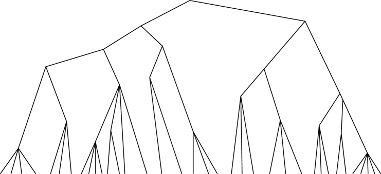
Figure 1: An example of a taxonomic tree of states in the case of an hierarchical breaking of the replica symmetry

The inequality (86) implies that the most relevant states form an ultrametric tree, i.e. they can be put on a tree in such a way that the states are on the branches of the tree and the distance among the states is the maximum level one has to cross for going from one states to an other. In other words the states of a system can be classified in a taxonomic way. The most studies possibilities are the following:

• All different states are at given distance $d$ one from the other and the taxonomy is rather trivial (one step replica symmetry breaking).

• The states have a continuous distribution and branching points exist at any level (continuous replica symmetry breaking). A suggestive drawing of how the tree may look like, if we draw only the finite number of branches that have weight larger than $\epsilon$, is shown in fig. (1). A careful analysis of the properties of the tree can be found in [31, 43].

Other distributions are possible, but they are less common or at least less studied.

5.5 The final result

In order to compute the free energy is useful to write down a formula for its value that is valid also in the case where there is a finite number of steps. After some thinking, we can check that the following expression (89) is a compact way to write the previous formulae for the free energy in terms of the function $x(q)$ (or $q(x)$). The expression for the free energy is a functional (a functional of the function $q[x]$) and it is given by:

$$\beta f[q(x)]={\beta^{2}\over 4}\left(1-\int_{0}^{1}q^{2}(x)\,dx\right)+f(0,0)$$ (89)

where the function $f(q,h)$ is defined in the strip $0\leq q\leq q_{EA}\equiv q_{K+1}$ and it obeys the non linear equation:

$$\dot{f}=-(f^{\prime\prime}+x(q)(f^{\prime})^{2})\ ,$$ (90)

where dots and primes mean respectively derivatives with respect to $q$ and $h$. The initial condition is

$$f(q,y)=\cosh(\beta m_{K}h)\ .$$ (91)

Now the variational principle tell us that the true free energy is greater than the maximum with respect to all function $q(x)$ of the previous functional. It is clear that a continuos function may be obtained as limit of a stepwise continuos function and this shows how to obtain the result for a continuos tree in a smooth way

Talagrand [20] is using on a cleaver the generalization of the bounds by Guerra [18] to systems composed by a two identical copies: he finally arrives to write also an upper bound for the free energy and to prove that they coincide. In this way after 24 years the following formula for the free energy of the SK model was proved to be true:

$$f=\max_{q(x)}f[q(x)]\ .$$ (92)

We have already remarked that the mathematical proof does not imply that the probability distribution of the descriptors is the one predicted by the physical theory. The main ingredient missing is the proof that the ultrametricity properties is satisfied. This is the crucial point, because ultrametricity and stochastic stability (which is known to be valid) completely fix the distribution. It is likely that the needed step would be to transform the estimates of [48] into rigorous bounds, however this is a rather difficult task. Maybe we have to wait other 24 years for arriving to the rigorous conclusion that the heuristic approach gave the correct results, although I believe that there are no serious doubts on its full correctness.

6 Bethe lattices

6.1 An intermezzo on random graphs

It is convenient to recall here the main properties of random graphs [49].

There are many variants of random graphs: fixed local coordination number, Poisson distributed local coordination number, bipartite graphs…They have the same main topological structures in the limit where the number ($N$) of nodes goes to infinity.

We start by defining the random Poisson graph in the following way: given $N$ nodes we consider the ensemble of all possible graphs with $M=\alpha N$ edges (or links). A random Poisson graph is a generic element of this ensemble.

The first quantity we can consider for a given graph is the local coordination number $z_{i}$, i.e. the number of nodes that are connected to the node $i$. The average coordination number $z$ is the average over the graph of the $z_{i}$:

$$z=\frac{\sum_{i=1,N}z_{i}}{N}\ .$$ (93)

In this case it is evident that

$$z=2\alpha\ .$$ (94)

It takes a little more work to show that in the thermodynamic limit ($N\to\infty$), the probability distribution of the local coordination number is a Poisson distribution with average $z$.

In a similar construction two random points $i$ and $k$ are connected with a probability that is equal to $z/(N-1)$. Here it is trivial to show that the probability distribution of the $z_{i}$ is Poisson, with average $z$. The total number of links is just $zN/2$, apart from corrections proportional to $\sqrt{N}$. The two Poisson ensembles, i.e. fixed total number of links and fluctuating total number of links, cannot be distinguished locally for large $N$ and most of the properties are the same.

Random lattices with fixed coordination number $z$ can be easily defined; the ensemble is just given by all the graphs with $z_{i}=z$ and a random graph is just a generic element of this ensemble .

One of the most important facts about these graphs is that they are locally a tree, i.e. they are locally cycleless. In other words, if we take a generic point $i$ and we consider the subgraph composed by those points that are at a distance less than $d$ on the graph , this subgraph is a tree with probability one when $N$ goes to infinity at fixed $d$. For finite $N$ this probability is very near to 1 as soon as

$$\ln(N)>A(z)\;d\ ,$$ (95)

$A(z)$ being an appropriate function. For large $N$ this probability is given by $1-O(1/N)$.

If $z>1$ the nodes percolate and a finite fraction of the graph belongs to a single giant connected component. Cycles (or loops) do exist on this graph, but they have typically a length proportional to $\ln(N)$. Also the diameter of the graph, i.e. the maximum distance between two points of the same connected component is proportional to $\ln(N)$. The absence of small loops is crucial because we can study the problem locally on a tree and we have eventually to take care of the large loops (that cannot be seen locally) in a self-consistent way. i.e. as a boundary conditions at infinity.

Before applying the problem will be studied explicitly in the next section for the ferromagnetic Ising model.

6.2 The Bethe Approximation in D=2

Random graphs are sometimes called Bethe lattices, because a spin model on such a graph can be solved exactly using the Bethe approximation. Let us recall the Bethe approximation for the two dimensional Ising model.

In the standard mean field approximation, one writes a variational principle assuming the all the spins are not correlated [5]; at the end of the computational one finds that the magnetization satisfies the well known equation

$$m=\mbox{th}(\beta Jzm)\ ,$$ (96)

where $z=4$ on a square lattice ($z=2d$ in $d$ dimensions) and $J$ is the spin coupling ($J>0$ for a ferromagnetic model). This well studied equation predicts that the critical point (i.e. the point where the magnetization vanishes) is $\beta_{c}=1/z$. This result is not very exiting in two dimensions (where $\beta_{c}\approx.44$) and it is very bad in one dimensions (where $\beta_{c}=\infty$). On the other end it becomes more and more correct when $d\to\infty$.

A better approximation can be obtained if we look to the system locally and we compute the magnetization of a given spin ($\sigma$) as function of the magnetization of the nearby spins ($\tau_{i}$, $i=1,4$). If we assume that the spins $\tau$ are uncorrelated, but have magnetization $m$, we obtain that the magnetization of the spin $\sigma$ (let us call it $m_{0}$) is given by:

$$m_{0}=\sum_{\tau}P_{m}[\tau]\mbox{th}(\beta J\sum_{i=1,4}\tau_{i})\ ,$$ (97)

where

$$P_{m}[\tau]=\prod_{i=1,4}P_{m}(\tau_{i}),\ \ \ \ \ \ P_{m}(\tau)=\frac{1+m}{2}\delta_{\tau,1}+\frac{1-m}{2}\delta_{\tau,-1}\ .$$ (98)

The sum over all the $2^{4}$ possible values of the $\tau$ can be easily done.

If we impose the self-consistent condition

$$m_{0}(m)=m\ ,$$ (99)

we find an equation that enables us to compute the value of the magnetization $m$.

This approximation remains unnamed (as far as I know) because with a little more work we can get the better and simpler Bethe approximation. The drawback of the previous approximation is that the spins $\tau$ cannot be uncorrelated because they interact with the same spin $\sigma$: the effect of this correlation can be taken into account ant this leads to the Bethe approximation.

Let us consider the system where the spin $\sigma$ has been removed. There is a cavity in the system and the spins $\tau$ are on the border of this cavity. We assume that in this situation these spins are uncorrelated and they have a magnetization $m_{C}$. When we add the spin $\sigma$, we find that the probability distribution of this spin is proportional to

$$\sum_{\tau}P_{m_{C}}[\tau])\exp\left(\beta J\sigma\sum_{i=1,4}\tau_{i}\right)\ .$$ (100)

The magnetization of the spin $\sigma$ can be computed and after some simple algebra we get

$$m=\mbox{th}\{z\;\mbox{arth}[\mbox{th}(\beta J)m_{C}]\}\ ,$$ (101)

with $z=4$.

This seems to be a minor progress because we do not know $m_{C}$. However we are very near the final result. We can remove one of the spin $\tau_{i}$ and form a larger cavity (two spins removed). If in the same vein we assume that the spins on the border of the cavity are uncorrelated and they have the same magnetization $m_{C}$, we obtain

$$m_{C}=\mbox{th}\{(z-1)\mbox{arth}[\mbox{th}(\beta J)m_{C}]\}\ .$$ (102)

Solving this last equation we can find the value of $m_{C}$ and using the previous equation we can find the value of $m$.

It is rather satisfactory that in 1 dimensions ($z=2$) the cavity equations become

$$m_{C}=\mbox{th}(\beta J)m_{C}\ .$$ (103)

This equation for finite $\beta$ has no non-zero solutions, as it should be.

The internal energy can be computed in a similar way: the energy density per link is given by

$$E_{link}={\mbox{th}(\beta J)+m_{C}^{2}\over 1+\mbox{th}(\beta J)m_{C}^{2}}\ .$$ (104)

We can obtain the free energy by integrating the internal energy as function of $\beta$.

In a more sophisticated treatment we write the free energy as function of $m_{C}$:

$${\beta F(m_{C})\over N}=F_{site}(m_{C})-\frac{z}{2}F_{link}(m_{C})\ ,\\$$ (105)

where $F_{link}(m_{C})$ and $F_{site}(m_{C})$ are appropriate functions [50]. This free energy is variational, in other words the equation

$${\partial F\over\partial m_{C}}=0$$ (106)

coincides with the cavity equation (102).

6.3 Bethe lattices and replica symmetry breaking

It should be now clear why the Bethe approximation is correct for random lattices. If we remove a node of a random lattice, the nearby nodes (that were at distance 2 before) are now at a very large distance, i.e. $O(\ln(N))$. In this case we can write

$$\langle\tau_{i_{1}}\tau_{i_{2}}\rangle\approx m_{i_{1}}m_{i_{2}}$$ (107)

and everything seems easy.

This is actually easy in the ferromagnetic case where in absence of magnetic field at low temperature the magnetization may take only two values ($\pm m$). In more complex cases, (e.g. antiferromagnets) there are many different possible values of the magnetization because there are many equilibrium states and everything become complex (as it should) because the cavity equations become equations for the probability distribution of the magnetizations [2].

I will derive the TAP cavity equations on a random Bethe lattice [28, 24, 26, 51] where the average number of neighbors is equal to $z$ and each point has a Poisson distribution of neighbors. In the limit where $z$ goes to infinity we recover the SK model.

Let us consider a node $i$; we denote by $\partial i$ the set of nodes that are connected to the point $i$. With this notation the Hamiltonian can be written

$$H=\frac{1}{2}\sum_{i}\sum_{k\in\partial i}J_{i,k}\sigma(i)\sigma(k)\,.$$ (108)

We suppose that for a given value of $N$ the system is in a state labeled by $\alpha$ and we suppose such a state exists also for the system of $N-1$ spins when the spin $i$ is removed. Let us call $m(i)_{\alpha}$ the magnetization of the spin $k$ and $m(k;i)_{\alpha}$ the magnetization of the spin $k$ when the site $i$ is removed. Two generic spins are, with probability one, far on the lattice: they are at an average distance of order $\ln(N)$; it is reasonable to assume that in a given state the correlations of two generic spins are small (a crucial characteristic of a state is the absence of infinite-range correlations). Therefore the probability distribution of two generic spins is factorized (apart from corrections vanishing in probability when $N$ goes to infinity) and it can be written in terms of their magnetizations.

We have already seen that the usual strategy is to write the equation directly for the cavity magnetizations. We obtain (for $l\in\partial i$):

$$m(i;l)=\tanh\left(\sum_{k\in\partial i;k\neq l}\mbox{artanh}(\tanh(\beta J_{i,k})m(k;i))\right)\ .$$ (109)

Following this strategy we remain with $Nz$ equations for the $Nz$ cavity magnetizations $m(i;k)$; the true magnetizations ($m(i)$) can be computed at the end using equation (109).

In the SK limit (i.e. $z\approx N$), it is convenient to take advantage of the fact that the $J$’s are proportional to $N^{-1/2}$ and therefore the previous formulae may be partially linearized; using the the law of large numbers and the central limit theorem one recovers the previous result for the SK model.

It is the cavity method, where one connects the magnetizations for a system of $N$ spins with the magnetizations for a system with $N-1$ spins. In absence of the spin $i$, the spins $\sigma(k)$ ($k\in\partial i$) are independent from the couplings $J_{i,k}$.

We can now proceed exactly as in SK model. We face a new difficulty already at the replica symmetric level: the effective field

$$h_{eff}=\sum_{k\in\partial i;k\neq l}\mbox{artanh}\left(\tanh(\beta J_{i,k})m(k;i)\right)$$ (110)

is the sum of a finite number of terms and it no more Gaussian also for Gaussian $J$’s. This implies that the distribution probability of $h_{eff}$ depends on the full probability distribution of the magnetizations and not only on its second moment. If one writes down the equations, one finds a functional equation for the probability distribution of the magnetizations ($P(m)$).

When replica symmetry is broken, also at one step level, in each site we have a probability distribution of the magnetization over the different states $Q(m)$ and the description of the probability distribution of the magnetization is now given by the probability distribution $P[Q(m)]$, that is a functional of the probabilities $Q(m)$ [24, 25, 51, 52, 53].

The computation becomes much more involved, but at least in the case of one step replica breaking (an sometimes at the two steps level) they can be carried up to the end. The one step approximation is quite interesting in this context, because there are optimization models in which it gives the exact results [52, 14]. A complete discussion of the stability of the one step replica approach can be found in [54].

7 Finite dimensions

7.1 General considerations

It is well known that mean field theory is correct only in the infinite dimensional limit. Usually in high dimensions it gives the correct results. Below the upper critical dimensions (that is 6 in the case of spin glasses) the critical exponents at the transition point change and they can be computed near to the upper critical dimensions using the renormalization group.

Sometimes the renormalization group is needed to study the behavior in the low temperature phase (e.g. in the $O(n)$ spin models), if long range correlations are present. A careful and complete analysis of spin glasses in the low temperature phase is still missing due to the extreme complexity of the corrections to the mean field approximation. Many very interesting results have been obtained [55], but the situation is still not clear. May be one needs a new approach, e.g starting to compute the corrections to mean field theory at zero temperature.

There are two different problems that we would like to understand much better:

• The value of the lower critical dimension.

• If the predictions of the mean field theory at least approximately are satisfied in three dimensions

These two problems will be addressed in the next two sections

7.2 The lower critical dimension

The calculation of free energy increase due to an interfaces is a well known method to compute the lower critical dimension in the case of spontaneous symmetry breaking. I will recall the basic points and I will try to apply it to spin glasses.

Generally speaking in the simplest case we can consider a system with two possible coexisting phases ($A$ and $B$), with different values of the order parameter,

For standard ferromagnets we may have ;

• A: spins up.

• B: spins down.

We will study what happens in a finite system in dimensions $D$ of size $M^{d}\ L$ with $d=D-1$.

We put the system in phase $A$ at $z=0$ and in phase $B$ at $z=L$. The free energy of the interface is the increase in free energy due to this choice of boundary conditions with respect to choosing the same phase at $z=0$ and $z=L$. In many cases we have that the free energy increase $\delta F(M,L)$ behaves for large $M$ and $L$ as:

$$\delta F(L,M)=M^{d}/L^{\omega}\ ,$$ (111)

where $\omega$ is independent from the dimension.

There is a lower critical dimension where the free energy of the interface is finite:

$$D_{c}=\omega+1\,,$$ (112)

and

$$\delta F(L,L)=L^{(D-D_{c})}\ .$$ (113)

Heuristic arguments, which sometimes can be made rigorous, tell us that when $D=\omega+1$, (the lowest critical dimension) the two phases mix in such a way that symmetry is restored.

In most cases the value of $\omega$ from mean field theory is the exact one and therefore we can calculate in this way the value of the lower critical dimension. The simplest examples are the ferromagnetic Ising model $\omega=0$ and the ferromagnetic Heisenberg model $\omega=1$.

For spin glasses the order parameter is the overlap $q$ and all values of $q$ in the interval $[-q_{EA},q_{EA}]$ are allowed. We consider two replicas of the same system described by a Hamiltonian:

$$H=H[\sigma]+H[\tau]\,,$$ (114)

where $H$ is the Hamiltonian of a a single spin glass. We want to compute the free energy increase corresponding to imposing an expectation value of $q$ equal to $q_{1}$ at $z=0$ and $q_{2}$ at $z=L$.

A complex computation gives [66] (for small $|q_{1}-q_{2}|$)

$$\delta F\propto ML(|q_{1}-q_{2}|/L)^{5/2}\propto L^{(D-5/2)}\ .$$ (115)

As a consequence, the naive prediction of mean field theory for the lower critical dimension for spontaneous replica symmetry breaking is $D_{c}=2.5$. I stress that these predictions are naive; corrections to the mean field theory are neglected. In known cases these kind of computations give the correct result,

A direct check of this prediction has never been done, however it quite remarkable that there are numerical results that strongly suggest that the lower critical dimension is really 2.5. Indeed a first method based on finding the dimension where the transition temperature is zero [56, 57], gives $D_{c}=2.491$. A more accurate method based on interpolating the value of a critical exponent [57] gives

$$D_{c}=2.4986\ ,$$ (116)

with an error of order $10^{-3}$ (my estimate).

It seem that this prediction for the lower critical dimension is well satisfied. It success implies that tree dimensional systems should be describe in the low temperature phase by the mean field approximation, although the correction could slowly vanish with the system size and the critical exponents could be quite different from the naive one, due to the fact three dimensions are only 0.5 dimensions above the lower critical dimensions. What happens in three dimension will be discussed in the next section.

7.3 The three dimensional case

Let us describe some of the equilibrium properties that has be computed or measured in the there dimensional case. We have to make a very drastic selection of the very vast literature, for a review see [6, 58].

All the simulations done with systems up $24^{3}$ [59] find that at low temperature at equilibrium a large spin glass system remains for an exponentially large time in a small region of phase space, but it may jump occasionally in a relatively short time to an other region of phase space (it is like the theory of punctuated equilibria: long periods of stasis, punctuated by fast changes). Example of the function $P_{J}(q)$, i.e. the probability distribution of the overlap among two equilibrium configurations, is shown in fig. (2) for two three dimensional samples.

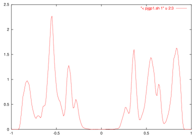
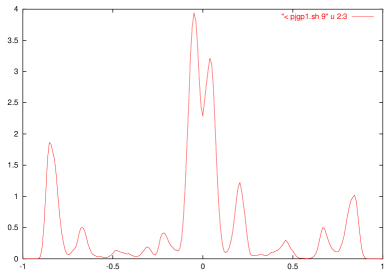
Figure 2: The function $P_{J}(q)$ for two samples (i.e two choices of $J$) for $D=3,\ L=16$ ($16^{3}$ spins) from [58].

We have defined $P(q)\equiv\overline{P_{J}(q)}$, where the average is done over the different choices of the couplings $J$, see fig. (3). We have seen that average is needed because the theory predicts (and numerical simulations also in three dimensions do confirm) that the function $P_{J}(q)$ changes dramatically from system to system. It is clear that the function remains non-trivial in the infinite volume limit.

In the mean field approximation the function $P(q)$ (and its fluctuations from system to system) can be computed analytically together with the free energy: at zero magnetic field $P(q)$ has two delta functions at $\pm q_{EA}$, with a flat part in between. The shape of the three dimensional function $P(q)$ is not very different from the one of the mean fields models.

The validity of the sum rules derived from stochastic stability (eqs. (61,63)) has been rather carefully verified [6]. This is an important test of the theory because they are derived in the infinite volume limit and there is no reason whatsoever that they should be valid in a finite system, if the system would be not sufficient large to mimic the behavior of the infinite volume system. There are also indication that both overlap equivalence [32, 33] and ultrametricity [67, 68] are satisfied, with corrections that goes to zero slowly by increasing the system size.

Figure 3: The function $P(q)=\overline{P_{J}(q)}$ after average over many samples (L=3…10) from [60].

Very interesting phenomena happen when we add a very small magnetic field. They are very important because the magnetic properties of spin glass can be very well studied in real experiment.

From the theoretical point of view we expect that order of the states in free energy is scrambled when we change the magnetic field [2]: their free energies differ of a factor $O(1)$ and the perturbation is of order $N$. Different results should be obtained if we use different experimental protocols:

• If we add the field at low temperature, the system remains for a very large time in the same state, only asymptotically it jumps to one of the lower equilibrium states of the new Hamiltonian.

• If we cool the system from high temperature in a field, we likely go directly to one of the good lowest free energy states.

Correspondingly there are two susceptibilities that can be measured also experimentally:

• The so called linear response susceptibility $\chi_{LR}$, i.e. the response within a state, that is observable when we change the magnetic field at fixed temperature and we do not wait too much. This susceptibility is related to the fluctuations of the magnetization inside a given state.

• The true equilibrium susceptibility, $\chi_{eq}$, that is related to the fluctuation of the magnetization when we consider also the contributions that arise from the fact that the total magnetization is slightly different (of a quantity proportional to $\sqrt{N}$) in different states. This susceptibility is very near to $\chi_{FC}$, the field cooled susceptibility, where one cools the system in presence of a field.

The difference of the two susceptibilities is the hallmark of replica symmetry breaking. In fig. (4) we have both the analytic results for the SK model [2] and the experimental data on metallic spin glasses [61]. The similarities between the two panels are striking.

Which are the differences of this phenomenon with a well known effect; i.e. hysteresis?

• Hysteresis is due to defects that are localized in space and produce a finite barrier in free energy. The mean life of the metastable states is finite and it is roughly $\exp(\beta\Delta F)$ where $\Delta F$ is a number of order 1 in natural units.

• In the mean field theory of spin glasses the system must cross barriers that correspond to rearrangements of arbitrary large regions of the system. The largest value of the barriers diverge in the thermodynamic limit.

• In hysteresis, if we wait enough time the two susceptibilities coincide, while they remain always different in this new framework if the applied magnetic field is small enough (non linear susceptibilities are divergent).

The difference between hysteresis and the this new picture (replica symmetry breaking) becoming clearer as we consider fluctuation dissipation relations during aging [10, 11, 12, 13, 69, 70], but this would be take to far from our study of equilibrium properties.

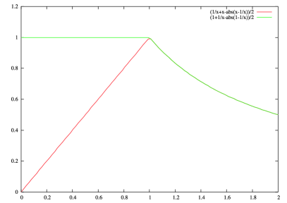
Figure 4: The two susceptibilities; upper panel, the analytic results in the mean field approximation [2]; lower panel, the experimental results for a metallic spin glass [61]

8 Some other applications

Some of the physical ideas that have been developed for spin glasses have also been developed independently by people who were working in the study of structural glasses. However in the fields of structural glasses there were no soluble models that displayed interesting behavior so most of the analytic tools and of the corresponding physical insight were firstly developed for spin glasses (for a review see for example [22]).

The two fields remained quite separate one from the other also because there was a widespread believe that the presence of quenched disorder (absent in structural glasses) was a crucial ingredient of the theory developed for spin glasses. Only in the middle of the 90’s it became clear that this was a misconception [71, 72] and it was realized that the spin glass theory may be applied also to systems where non-intrinsic disorder is present (e.g. hard spheres).

This became manifest after the discovery of models where there is a transition from a high temperature liquid phase to a low temperature glassy phase (some of these models at low temperature have two phases, a disorder phase and an ordered, crystal phase). Spin glass theory was able to predict the correct behavior both at high and at low temperature [71, 72, 73].

There are many other problems where these ideas have been used. In the past there has been a great interest in applying them to problems with a biological flavor, like the computation of the optimal performance of associative memories based on neural networks [74]. Also learning abilities of simpler objects like the perceptrons can be computed.

In recent years they have been widely used in the field of combinatorial optimization problems and constraint satisfaction, but this will be discussed elsewhere in this volume [14].

9 Conclusions

From the retrospective point of view it may seem extraordinary the amount of new ideas that has been necessary in order to understand in depth the basic properties of spin glasses and other glassy system. A strong effort should be done in order to have better quantitative predictions and a more precise comparison between theory and experiments.

I ma convinced that there are still many very interesting surprises that will come from a careful study of spin glasses (and related problem) and it is quite likely that the most exciting result will come from an area I am not able to indicate. I am very curious to see the future of the field.

Appendix I: A useful little theorem

In this appendix we want to prove a useful little theorem [24], which may be useful in many contests.

Theorem: consider a set of $M(\gg 1)$ iid random free energies $f_{\alpha}$, ($\alpha\in\{1\ldots M\}$) distributed with the exponential density eq. (67) , and a set of $M$ positive numbers $a_{\alpha}$. Then, neglecting terms which go to zero when $M$ goes to infinity, the following relation holds:

$$\langle\ln\left({\sum_{\alpha}a_{\alpha}\exp(-\beta f_{\alpha})\over\sum_{\alpha}\exp(-\beta f_{\alpha})}\right)\rangle_{f}$$ (117)

$$\equiv\langle\ln\left(\sum_{\alpha}w_{\alpha}a_{\alpha}\right)\rangle_{f}={1\over x}\ln\left({1\over M}\sum_{\alpha}a_{\alpha}^{x}\right)\,,$$

where $\langle\cdot\rangle_{f}$ denotes an average over the distribution of $f$.

Corollary 1: In the same conditions as the theorem, for any set of $M$ real numbers $b_{\alpha}$, one has:

$$\left\langle{\sum_{\alpha}a_{\alpha}b_{\alpha}\exp(-\beta f_{\alpha})\over\sum_{\alpha}a_{\alpha}\exp(-\beta f_{\alpha})}\right\rangle_{f}={\sum_{\alpha}a_{\alpha}^{x}b_{\alpha}\over\sum_{\alpha}a_{\alpha}^{x}}\ .$$ (118)

Corollary 2: If the numbers $a_{\alpha}$ are $M$ iid positive random variables, such that the average of $a^{x}$ exists, which are uncorrelated with the $f_{\alpha}$, then one has:

$$\left\langle\ln\left({\sum_{\alpha}a_{\alpha}\exp(-\beta f_{\alpha})\over\sum_{\alpha}\exp(-\beta f_{\alpha})}\right)\right\rangle_{f}\equiv\left\langle\ln\left(\sum_{\alpha}w_{\alpha}a_{\alpha}\right)\right\rangle_{f}={1\over x}\ln\left(\langle a_{\alpha}^{x}\rangle_{a}\right)\ ,$$ (119)

where $\langle\cdot\rangle_{a}$ denotes an average over the distribution of $a$.

Remark: We notice that in the two limits $x\to 0$ and $x\to 1$ the equations can be simply understood:

• In the limit $x=0$, in a typical realization of the random free energies, only one weight $w$ is equal to one and all the others are zero. Averaging over the realizations of free energies amounts to spanning uniformly the set of indices of this special non zero weight.

• In the limit $x=1$ the number of relevant $w$ goes to infinity and each individual contribution goes to zero. An infinite number of term is present in the l.h.s. of eq. (Appendix I: A useful little theorem) and the r.h.s. of the eq. (Appendix I: A useful little theorem) becomes $\ln\left[(1/M)\sum_{\alpha}a_{\alpha}\right]$, as it should.

References

- [1] Anderson P.W. (1983), in Ill condensed matter, eds Balian R., Maynard R and Toulouse G., (North-Holland, Berlin) pp. 159-259.
- [2] Mézard, M., Parisi, G. and Virasoro, M.A. (1987) Spin Glass Theory and Beyond, (World Scientific, Singapore).
- [3] Parisi G. (1992) Field Theory, Disorder and Simulations, (World Scientific, Singapore).
- [4] Newman C.M. and Stein D.L. (1996) J. Stat. Phys. 82, 1113.
- [5] See for example: Parisi G. Statistical Field Theory (Academic Press, New York) 1987.
- [6] Marinari E., Parisi G., Ricci-Tersenghi F., Ruiz-Lorenzo J. and Zuliani F. (2000) J.Stat. Phys 98, 973.
- [7] G. Parisi, Physica Scripta 35, 123 (1987).
- [8] G. Parisi, Phil. Mag. B 71, 471 (1995).
- [9] Bouchaud J.-P. (1992) J. Phys. France 2 1705.
- [10] Cugliandolo L.F. and Kurchan J.(1993) Phys. Rev. Lett. 71, 173.
- [11] Cugliandolo L.F. and Kurchan J.(1994) J. Phys. A: Math. 27, 5749.
- [12] Franz S. and Mézard M. (1994) Europhys. Lett. 26, 209.
- [13] Franz S., Mézard M., Parisi G., Peliti L. (1999), J. Stat. Phys. 97 459.
- [14] See for example the lectures by R. Monasson and A. Montanari at this school.
- [15] Guerra F. (1997) Int. J. Phys. B, 10, 1675.
- [16] Aizenman M. and Contucci P. (1998) J. Stat. Phys, 92, 765.
- [17] Parisi G. Int. Jou. Mod. Phys. B, 18, 733-744, (2004).
- [18] Guerra F. (2002) Comm. Math. Phys. 233 1.
- [19] Aizenman M. , Sims R. , Starr S. L.(2003) Phys. Rev. B 68, 214403.
- [20] Talagrand M. (2006), Ann. of Math., 163 221.
- [21] Sherrington D. and Kirkpatrick S.(1975) Phys. Rev. Lett., 35, 1792.
- [22] G. Parisi in Les Houches Summer School - Session LXXVII: Slow relaxation and non equilibrium dynamics in condensed matter, ed. by J.-L. Barrat, M.V. Feigelman, J. Kurchan, and J. Dalibard, Elsevier 2003.
- [23] Viana L. and Bray A. J. (1985) J. Phys. C18 3037.
- [24] Mézard M. and Parisi G.(2001) Eur.Phys. J. B 20 217.
- [25] Mézard M. and Parisi G.(2003) J. Stat. Phys 111 1.
- [26] Franz S. and Leone M. (2003) J. Stat. Phys 111 535.
- [27] Edwards S. and Anderson P. J.(1975) J. Phys F5 965.
- [28] Thouless D.J.,Anderson P. A. and Palmer R. G. (1977) Phil. Mag. 35, 593.
- [29] R.L. de Almeida, D.J. Thouless, J. Phys. A 11 (1978) 983.
- [30] D. Kastler and D. W. Roberts, Comm. Math. Phys. 3, 151 (1965).
- [31] Ruelle D. (1988) Commun. Math. Phys. 48, 351.
- [32] E. Marinari, G. Parisi Phys. Rev. Lett. 86, 3887-3890 (2001).
- [33] P. Contucci, C. Giardinà, C. Giberti, C. Vernia Phys. Rev. Lett. 96, 217204 (2006).
- [34] P. Contucci, J. Phys. A: Math. Gen. 36, 10961, (2003); P. Contucci, C. Giardinà, Jour. Stat. Phys. to appear math-ph/05050 (2005).
- [35] G. Parisi in Les Houches Summer School - Session LXXXIII: Mathematical Statistical Physics, ed. by A. Bovier, F. Dunlop, F. den Hollander and A. van Enter, Elsevier 2006.
- [36] I. Giardina’s contribution to this school.
- [37] Iniguez D., Parisi G. and Ruiz-Lorenzo J.J.(1996) J.Phys. A29 4337.
- [38] Parisi G. (2003) J. Phys. A 36 10773.
- [39] G.Parisi (2004) Europhys. Lett. 65, 103.
- [40] J. Kurchan, G.Parisi and M.A. Virasoro J. Phys. I France 3 (1993) 1819.
- [41] M.E. Ferrero and M.A. Virasoro J. Phys. I France 4 (1994) 1819.
- [42] G. Parisi (1994) in Perspectives on Biological Complexity, eds. O.T. Solbrig and G. Nicolis, (IUBS,Paris) pp 87-121.
- [43] Parisi G. (1993) J. Stat. Phys. 72, 857-872 .
- [44] G. Parisi and F. Ricci-Tersenghi J. Phys. A 33 113 (2000).
- [45] G. Parisi M. Talagrand C.R.A.S. 339, 2004, 306-306
- [46] Franz S. and Parisi G. (2000) Europ J. Phys 18 1434.
- [47] D.Ruelle, Commun. Math. Phys. 108, 225 (1987).
- [48] S. Franz, G Parisi, M.A. Virasoro, .Europhys. Lett. 22, 405 (1993).
- [49] P. Erdös and A. Rènyi, Publ. Math. (Debrecen) 6, 290 (1959).
- [50] Katsura S., Inawashiro S. and Fujiki S., Physica 99A (1979) 193.
- [51] G. Parisi On local equilibrium equations for clustering states cs.CC/0212047 (2002).
- [52] Mézard M., Parisi G. and Zecchina R. (2002) Science 297, 812.
- [53] G.Parisi On the survey-propagation equations for the random K-satisfiability problemcs.CC/0212009 (2002).
- [54] A. Montanari, G Parisi, F Ricci-Tersenghi, J. Phys. A 37 2073 (2004).
- [55] T. Temesvari Replica symmetric spin glass field theory cond-mat/0612523 and reference therein.
- [56] G. Parisi, P. Ranieri, F. Ricci-Tersenghi, and J. J. Ruiz-Lorenzo, J. Phys. A 30, 7115 (1997).
- [57] S. Boettcher Stiffness of the Edwards-Anderson Model in all Dimensions cond/mat 0508061.
- [58] Marinari E., Parisi G. and Ruiz-Lorenzo J.J. (1998) in Spin Glasses and Random Fields, ed. P. Young (World Scientific, Singapore ) pp. 58.
- [59] L. Gnesi, R. Petronzio and F. Rosati Evidence for Frustration Universality Classes in 3D Spin Glass Models cond-mat/0208015.
- [60] Marinari E., Zuliani F. (1999) J. Phys. A 32, 7447-7461.
- [61] C. Djurberg, K. Jonason and Nordblad P. (1998) Eur. Phys. J. B 10, 15.
- [62] Marinari E., Parisi G., J. Ruiz-Lorenzo, and F. Ritort (1996) Phys. Rev. Lett. 76, 843.
- [63] Joh Y.G. , Orbach R. , Wood G.G. , Hammann J. , Vincent E. (1999) Phys. Rev. Lett. 82, 438.
- [64] Marinari E., Parisi G. , Ricci-Tersenghi F. and Ruiz-Lorenzo J.J. (1998) J. Phys. A 31, 2611.
- [65] Parisi G., Ricci-Tersenghi F., and Ruiz-Lorenzo J.J. (1999) Eur. Phys. J. B 11, 317-325.
- [66] S. Franz, G Parisi, M.A. Virasoro, .J. Phys. France 4, 1657 (1994).
- [67] A. Cacciuto, E. Marinari, G. Parisi J. Phys. A: Math. Gen 30 L263-L269 (1997).
- [68] P. Contucci, C. Giardinà, C. Giberti, G. Parisi, C. Vernia Ultrametricity in the Edwards-Anderson Model, cond-mat/0607376.
- [69] D. Hérisson and M. Ocio, Phys. Rev. Lett. 88, 257202 (2002).
- [70] G.Parisi PNAS 103 7948 (2006).
- [71] Marinari E., Parisi G. and Ritort F. (1994) J. Phys. A 27 , 7647.
- [72] Bouchaud J.-P. and Mézard M. (1994) J. Physique 4 1109.
- [73] Degli Esposti M., Giardinà C., Graffi S., Isola S. (2001) J. Stat. Phys. 102, 1285.
- [74] See for example Amit D.J. (1989) Modeling Brain Functions, (Cambridge University Press, Cambridge).