The discovery of a massive supercluster at z = 0.9 in the UKIDSS DXS

Abstract

We analyse the first publicly released deep field of the UKIDSS Deep eXtragalactic Survey (DXS) to identify candidate galaxy over-densities at $z\sim 1$ across $\sim$1 sq. degree in the ELAIS-N1 field. Using $I-K$,$J-K$ and $K-3.6\mu$m colours we identify and spectroscopically follow-up five candidate structures with Gemini/GMOS and confirm they are all true over-densities with between five and nineteen members each. Surprisingly, all five structures lie in a narrow redshift range at $z=0.89\pm 0.01$, although they are spread across 30 Mpc on the sky. We also find a more distant over-density at $z=1.09$ in one of the spectroscopic survey regions. These five over-dense regions lying in a narrow redshift range indicate the presence of a supercluster in this field and by comparing with mock cluster catalogs from $N$-body simulations we discuss the likely properties of this structure. Overall, we show that the properties of this supercluster are similar to the well-studied Shapley and Hercules superclusters at lower redshift.

Figure 1: The $J-K$, $I-K$ and $K-3.6\mu$m colour-magnitude plots for each cluster. The colour-magnitude diagrams represent a 1.5 arcminute region around each cluster. The dashed lines show the limits used to select candidate cluster members via the red sequence. We identify the spectroscopically confirmed $z=$0.89 cluster members (filled squares), as well as the fore-/background galaxies (filled circles). In the DXS4 field we identify separately the members of the higher redshift structure in this field (at $z=1.09$). Note also that some spectra were taken for objects outside the colour-magnitude limits (marked as dashed boxes) to fully populate the GMOS masks.

1 Introduction

The structure and evolution of clusters of galaxies and their constituent substructures provides a powerful test of our understanding of both the growth of large scale structure and dark matter in the Universe. In the current hierarchical paradigm of structure formation, massive galaxy clusters arise from the extreme tail in the distribution of density fluctuations, so their number density depends critically on cosmological parameters. One of the remarkable successes of the $\Lambda$-CDM paradigm is the match to the number density, mass and evolution of clusters of galaxies out to $z\sim 0.5$–1 (Jenkins et al., 2001; Evrard et al., 2002). However, due to the very limited number of clusters known at $z\mathrel{\raise 1.50696pt\hbox{$\scriptstyle>$}\kern-6.00006pt\lower 1.72218pt\hbox{{$\scriptstyle\sim$}}}1$ (where the number density is most sensitive to the assumed cosmology), the full power of the comparisons to theoretical simulations has not yet been exploited.

The paucity of clusters known at $z\mathrel{\raise 1.50696pt\hbox{$\scriptstyle>$}\kern-6.00006pt\lower 1.72218pt\hbox{{$\scriptstyle\sim$}}}1$ stems from the limitations of current survey methods. For instance, optical colour-selection of clusters (Couch et al., 1991; Gladders & Yee, 2000), which relies on isolating the 4000Å break in the spectral energy distributions of passive, red early-type galaxies (the dominant population in local clusters) becomes much less effective at $z\mathrel{\raise 1.50696pt\hbox{$\scriptstyle>$}\kern-6.00006pt\lower 1.72218pt\hbox{{$\scriptstyle\sim$}}}0.7$ where this feature falls in or beyond the $i$-band, in a region of declining sensitivity of silicon-based detectors. Recent progress has been made in identifying clusters using X-ray selection with Chandra and XMM-Newton (Romer et al., 2001; Rosati et al., 2002; Mullis et al., 2005) and these studies have identified galaxies clusters out to $z\sim 1.5$ (Stanford et al., 2006; Bremer et al., 2006). However, the X-ray gas in these clusters appears more compact than for comparable systems at lower redshifts and hence there are concerns that the accurate comparison of cluster properties with redshift required to constrain cosmological parameters could be subject to potential systematic effects related to the thermal history on the intra-cluster medium. Thus a complimentary technique for cluster selection is required.

One solution to this problem is to extend the efficient optical colour-selection method beyond $z\mathrel{\raise 1.50696pt\hbox{$\scriptstyle>$}\kern-6.00006pt\lower 1.72218pt\hbox{{$\scriptstyle\sim$}}}0.7$ using near-infrared detectors (Hirst et al., 2006). This approach has been impressively demonstrated by Stanford et al. (2006) who find a $z=1.45$ cluster in the NOAO-DW survey selected from optical-near-infrared colours. The commissioning of the new wide-field WFCAM camera on UKIRT provides the opportunity to significantly expand deep panoramic surveys in the near-infrared. The Deep eXtragalactic Survey (DXS) is a component within the UK Infrared Deep Sky Survey (UKIDSS) (Warren et al., 2007) with the aim of imaging an area of 35 square degrees at high Galactic latitudes in the $J$- and $K$-band filters to a depth $J_{AB}$=23.2 and $K_{AB}$=22.7 respectively. The principal goals of the DXS include measuring the abundance of galaxy clusters at $z\sim 1$–1.5, measuring galaxy clustering at $z\sim 1$ and measuring the evolution of bias. This paper presents the first results from a spectroscopic follow-up of five high redshift galaxy cluster candidates identified in the DXS Early Data Release (EDR; Dye et al. 2006).

The structure of this paper is as follows. In §2 we describe the data on which our analysis is based: a combination of optical, near- and mid-infrared imaging with Subaru, UKIRT and Spitzer which is used to select cluster candidates and the follow-up Gemini/GMOS spectroscopy. In §3 we present an analysis of the cluster properties. We discuss these and give our conclusions in §4. Unless otherwise stated, we assume a cosmology with $\Omega_{m}$=0.27, $\Lambda=$0.73 and $H_{0}$=70$\,\hbox{km}\,\hbox{s}^{-1}$ Mpc^-1. All magnitudes are given in the AB system.

2 Observations and Reduction

We utilise the UKIDSS-DXS EDR for the ELAIS-N1 region which covers a contiguous area of $0.86^{\circ}\times 0.86^{\circ}$ centred on $\alpha=16$ 11 14.400; $\delta=+54$ 38 31.20 (J2000). The survey data products for this region reach 5-$\sigma$ point source limits of $J_{AB}=22.8$–23.0 and $K_{AB}=22.9$–23.1. To complement these observations we exploit deep $I$-band imaging obtained with Suprime-Cam on Subaru Telescope. These observations cover the entire ELAIS-N1/DXS field and are described in Sato et al. 2007 (in preparation) and reach a 5-$\sigma$ point-source limit of $I_{AB}=26.2$. As part of the Spitzer Wide-area InfraRed Extragalactic (SWIRE) survey (Lonsdale et al., 2003), the ELAIS-N1 region was also imaged in the IRAC (3.6, 4.5, 5.8 and 8.0$\mu$m) bands as well as at 24$\mu$m with MIPS. These catalogs are described in Surace et al. (2004).

2.1 Optical-Infrared matching

In order to efficiently select cluster candidates, accurate colours are required for galaxies in the coincident regions of the DXS, Subaru and SWIRE. The DXS catalogue was constructed using SExtractor (Bertin & Arnouts, 1996) with a detection threshold of 2$\sigma$ in at least five pixels. Objects which lay in the halo or CCD bleed of a bright star were also removed before the final catalog was constructed. This catalogue was then matched to the optical catalogue, with the closest match within $1^{\prime\prime}$ being used. During the first pass cross-correlation the average offsets between the optical and near-infrared catalogues was $\Delta\alpha=0.33\pm 0.05^{\prime\prime}$, $\Delta\delta=-0.20\pm 0.04^{\prime\prime}$ (i.e. the optical sources were offset to the south-east of the near-infrared sources, which are tied to FK5 through 2MASS stars, Dye et al. 2006). This systematic offset was removed from the optical catalog and the cross-correlation recalculated resulting in an rms offset of $\sim 0.1^{\prime\prime}$. Since accurate colours were required in order to select cluster candidates, we extracted 2^′′ aperture magnitudes from the optical and near-infrared catalogs. In both cases, the magnitude zero-points were calculated using 2^′′ photometry of (unsaturated) stars in the field.

The near-infrared and mid-infrared catalogs were cross-correlated in exactly the same way as above, with a systematic offset between the mid-infrared and near-infrared sources of $\Delta\alpha=-0.30\pm 0.05^{\prime\prime}$, $\Delta\delta=0.33\pm 0.04^{\prime\prime}$, which again was removed before a second pass cross-correlation was performed.

2.2 Cluster Selection

As this was a pilot study, we choose to identify candidate high-redshift galaxy clusters in three ways. First, we searched for the sequence of passive red galaxies in high-redshift clusters by selecting galaxies from photometric catalogue in the $(J-K)$–$K$ and $(I-K)$–$K$ colour-magnitude space. We first identified candidates using slices of $\Delta(J-K)_{AB}=0.4$ stepped between $(J-K)_{AB}=0$–2.5. This selection includes a small correction for the tilt of the colour-magnitude relation for early type galaxies of $d(J-K)_{AB}/dK_{AB}=-0.025$. Consecutive slices overlapped by 0.2 magnitudes to ensure that no sequence was omitted. Each position in the resulting spatial surface density plot for a colour slice was then tested for an over-density using consecutively larger apertures from 0.01 to 0.05 degrees (corresponding to approximately 250 kpc to 1 Mpc at $z=1$). If the over-density in the central aperture was $\geq 3\sigma$ above the background and the density decreased with increasing aperture radius then a region was marked as a candidate cluster. A similar procedure was carried out using the $(I-K)$–$K$ colour-magnitude space to refine the selection of cluster candidates. Independently, we identified cluster candidates by identifying peaks in the surface density in $K_{AB}-3.6\mu$m colour space (using an approximate colour cut of $K_{AB}-3.6\mu{\rm m}>0.3$ which should be efficient at selecting elliptical at $z\sim$1). Having defined these cluster candidates, we checked that each of these met the selection criterion recently used by van Breukelen et al. (2006) (which is based on a projected friends of friends algorithm). Using these three selection criteria we identified fifteen candidates, of which eight were identified using all three criteria. Five of the most promising eight cluster candidates (which showed the tightest colour-magnitude sequences and a clear over-density of red objects), were then targeted for spectroscopic follow-up. In Fig. 1 we show the colour-magnitude diagrams for a 1.5 arcminute region around each of the over-density peaks which were spectroscopically targeted (the dashed boxes in Fig. 1 show the colours used to select the cluster candidates).

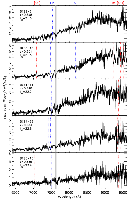
Figure 2: Example spectra of the cluster members from the GMOS spectroscopy. The example spectra cover the range of $I$-band magnitude of the spectroscopic sample ($I\sim$21.0–23.5). The dashed lines mark the expected position of the emission and absorption lines of [Oii]3727, Ca H&K, G-band, H$\beta$ and [Oiii]4959,5007. The grey region shows the position of the uncorrected telluric absorption band.

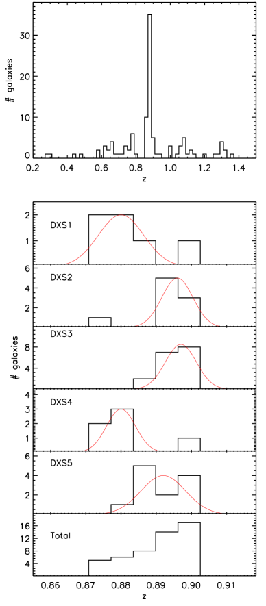
Figure 3: Top: The total redshift distribution for the five regions targeted in our spectroscopic follow-up. This clearly shows the strong overdensity in these regions at $z=0.9$. Middle: The redshift histograms for each individual cluster with the mean and 1-$\sigma$ scatter overplotted (using the method described in §3.2). The Bottom panel shows the redshift distribution for the whole sample on the same velocity scale. For reference the bin size in the lower panels is 1000 km s^-1 (in the rest frame of the cluster).

2.3 GMOS Spectroscopy

Spectroscopic follow-up observations of five candidate overdense regions were taken with the Gemini Multi-Object Spectrograph (GMOS) on Gemini-North between 2006 May 23 and June 18 U.T. in queue mode. As our target clusters were expected to be at $z\sim 1$ we placed a strong emphasis on good sky subtraction, to identify weak features in the presence of strong and structured sky emission.

For this reason we employed the Nod & Shuffle mode of GMOS. In Nod & Shuffle, the object and background regions are observed alternately through the same regions of the CCD by nodding the telescope. In between each observation the charge is shuffled on the CCD by a number of rows corresponding to the the centre-to-centre spacing into which each slit is divided. Each alternate block is masked off so that it receives no light from the sky but acts simply as an image store. The sequence of object and background exposures can be repeated as often as desired and at the end of the sequence, the CCD is read, incurring a read-noise penalty only once (see Glazebrook & Bland-Hawthorn 2001 for further details of this general approach). For each spectrum, the two spectra block are identified and subtracted to achieve Poisson-limited sky subtraction.

For our observations we micro-step the targets in the 3.2^′′ long slits by 1.5^′′ every 30 seconds. We used the OG515 filter in conjunction with the R400 grating and a central wavelength of 840 nm which results in a wavelength coverage of $\sim 580$–1100 nm. The spectral resolution in this configuration is $\lambda/\Delta\lambda\sim 1700$ and the slit width was 1.0^′′. To counter the effects of bad pixels and the GMOS chip gaps, the observations were taken with two wavelength configurations, each comprising two 2.8-ks exposures at central wavelengths of 840 nm and 850 nm respectively. Each of the five masks was observed for a total of 3.2 hours in $\mathrel{\raise 1.50696pt\hbox{$\scriptstyle<$}\kern-6.00006pt\lower 1.72218pt\hbox{{$\scriptstyle\sim$}}}0.7^{\prime\prime}$ seeing and photometric conditions. In total 134 galaxies are included on these five masks and we list the positions and photometric properties ($IJK$ and the IRAC/MIPS bands) of these in Tables 2&3.

To reduce the data, we first identified charge traps from a series of dark exposures taken during the run and used these to mask bad pixels. We extract the nod and shuffle regions from the data frames and then mosaiced the three GMOS CCDs. The frames were then flat-fielded, rectified, cleaned and wavelength calibrated using a sequence of Python routines (Kelson, priv. com.). The final two-dimensional mosaic was generated by aligning and median combining the reduced two-dimensional spectra using a median with a 3-$\sigma$ clip to remove any remaining cosmic rays or defects. For flux calibration, observations of BD+28d4211 were taken, however, no tellurics were taken and so we have not attempted to correct for the $A$-band absorption at 7600Å although this is unimportant for deriving redshifts in any of our spectra. While flux-calibration and response correction are not necessary for redshift determination via cross-correlation, we perform these steps in order to present the spectra in Fig. 2.

3 Analysis

Table 1.

Properties of the Cluster Candidates

Cluster	R.A.	Dec.	nslits	ncl	$z$	$\sigma$	$\sigma$’
	(J2000)					(km s-1)	(km s-1)
DXS1	16 08 27.0	+54 35 47	26	5	0.8800[19]	$1030\pm 270$	640$\pm$330
DXS2	16 08 26.9	+54 45 12	25	9	0.8960[19]	$700\pm 230$	440$\pm$170
DXS3	16 09 05.7	+54 57 23	29	17	0.8970[14]	$730\pm 220$	570$\pm$160
DXS4a	16 13 01.7	+54 46 06	…	5	0.8800[12]	$660\pm 180$	470$\pm$230
DXS4b			25	8	1.0918[14]	$1200\pm 340$
DXS5	16 10 43.6	+55 01 35	29	12	0.8920[20]	$1000\pm 290$	550$\pm$240

Table 1: Names, central positions and properties of the spectroscopic sample. n_slits and n_cl denote the number of spectroscopic slits on the mask and the number of confirmed cluster member respectively. $\sigma$ is the velocity dispersion of the spectroscopic sample and $\sigma$’ is the velocity dispersion after removal of substructure. The values in the [] denote the errors in the last decimal place.

3.1 Redshift determination and velocity dispersions

For redshift determination we first attempt to identify strong emission or absorption features in the spectra including [Oii]$\lambda$3726.2,3728.9 emission, the 4000Å break, Ca H&K absorption at $\lambda$3933.44,3969.17 or the G-band at $\lambda$4304.4. From the sample of 134 galaxies with spectroscopic observations, 111 yielded secure redshifts, with only 23 unidentifiable, giving a 85% success rate. As expected for absorption-line spectroscopy, the non-detections can in large part be attributed to optical faintness: the median $I_{AB}$ magnitude of the 111 galaxies with secure redshifts is $22.15\pm 0.2$, whereas for the galaxies without redshifts the median magnitude was $I_{AB}=22.65\pm 0.4$. The measured redshifts for all sources are listed in Tables 2&3.

Having identified an approximate redshift for a galaxy we compute a robust velocity by cross-correlating each the spectrum with an elliptical galaxy template spectrum. For the template we use solar metallicity, 1 Gyr burst models with ages of 3,5 or 7 Gyr from Bruzual & Charlot (2003). The errors on the redshifts are determined from the shape of the cross-correlation peak and the noise associated with the spectrum and are typically in the range 30–150 km s^-1. We present typical example spectra from each of the masks in Fig. 2 and report the errors on the redshifts of the individual candidate cluster members in Table 2.

Figure 3 shows the redshift distribution for all galaxies in our sample. We see that the vast majority of the spectroscopic sources lie in a narrow redshift range at $z\sim 0.9$. This indicates that most of the galaxies we have selected lie within the overdense regions we targeted and that these structures themselves appear to form a coherent structure across the whole survey region.

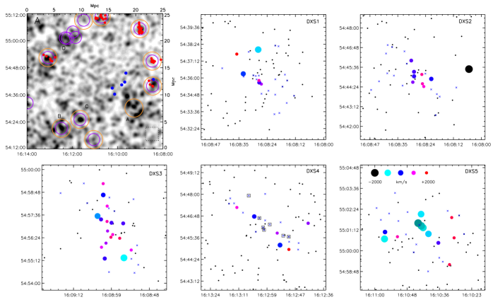
Figure 4: Panel A: Colour-selected surface density map of the ELAIS-N1 region based on the $I-K$, $J-K$ and $K$-3.6$\mu$m colours used to select galaxy clusters (the cluster candidate selection is described in §2). The image is smoothed with a Gaussian kernel with a FWHM of $60^{\prime\prime}$ (420 kpc at $z=0.9$). The large open circles represent the cluster candidate colour selection using $J-K$ (large circles) and $K$-3.6$\mu$m (slightly smaller) colours. The dashed square box in the bottom right hand corner shows the size of the GMOS field of view. For the five regions targeted in our GMOS observations we mark the individual galaxies which are known to be members and in addition we plot those galaxies from the literature which lie between $z=0.870$ and $z=0.915$. The cluster candidates marked A-D have colour-magnitude sequences consistent with the z=0.89 supercluster. It is clear that the supercluster potentially spans the whole field (the most prominent region is at 16:10:09, 54:25:00) and beyond. Panels DXS1-5: The spatial distribution of the galaxies within in each of the five over-dense regions selected for spectroscopic study. We plot the positions of all of the galaxies which meet our colour-selection (see §2.2) and we identify those which are spectroscopically confirmed as cluster members or non-members. For the members, the sizes and colours of the symbols denote the rest-frame velocity offset with respect to the cluster redshift given in Table 1 (on a velocity scale from $-2000$ to $+2000$ km s^-1). In addition, in the DXS4 field we identify the members of the background $z=1.09$ structure.

To calculate the membership of the structure in each field, we have followed the iterative method used by Lubin et al. (2002). Initially we estimated the central redshift for the overdensity, and select all other galaxies with $\Delta z<\pm 0.06$ in redshift space. We then calculated the bi-weight mean and scale of the velocity distribution (Beers et al., 1990) which correspond to the central velocity location, $v_{c}$, and dispersion, $\sigma_{v}$ of the cluster. We used this to calculate the relative radial velocities in the restframe: $\Delta v=c(z-z_{c})/(1+z_{c})$. The original distribution was revised, and any galaxy that lies $>3\sigma_{v}$ away from $v_{c}$, or has $|\Delta{v}|>3500$ km s^-1 was rejected from the sample and the statistics were re-calculated. The final solution is achieved when no more galaxies are removed by the iterative rejection. The results are presented in Table 1, with 1-$\sigma$ errors on the cluster redshift and dispersion corresponding from $10^{3}$ bootstrap re-samples. We plot the redshift histograms for the structures in each field in Figure 3 along with a Gaussian curve showing the measured mean redshift and velocity dispersion.

The most striking result from these histograms is the discovery that all five structures lie within 3000 km s^-1 of each other even though they are spread across nearly a degree on the sky (approximately 30 Mpc in projection). This strongly suggests that this field intercepts a “supercluster” like structure at $z=0.9$ – we discuss the posterior likelihood of this in §4 and next discuss the the properties of the individual structures.

3.2 Searching for Substructures

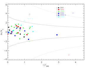
Figure 5: The cluster membership technique of Carlberg, Ellingson & Yee (1997) applied to our cluster sample. The solid curve denotes the 3$\sigma$ contour of the mass model; the dashed curve is the 6$\sigma$ contour. The filled symbols denote galaxies which lie within the 3$\sigma$ contours whilst the open symbols denote galaxies which lie outside the 3$\sigma$ contours. This test shows that significant substructure is evident in DXS5, with outliers also evident in DXS1, 2 & 3. Restricting our analysis to the galaxies within the central 3$\sigma$ limits we derive velocity dispersions for the whole sample of 540$\pm$100$\,\hbox{km}\,\hbox{s}^{-1}$.

We list the centres of the structures identified from our dynamical analysis in Table 1, along with the number of members, the mean redshift and the estimate of the velocity dispersion for each structure. Since the central positions and redshifts of the clusters are not well constrained we define the central velocity as the median redshift in the cluster and determine the centre of the cluster from the peak in the cluster surface density plot (Fig. 4). The uncertainties on the velocity dispersions are derived from bootstrap resampling the observed sample of members. Measuring the velocity dispersions from clusters with $\sim$10 members is particularly difficult, and in the rest-frame, the cluster velocity dispersions are unusually high ($\sim$1000$\,\hbox{km}\,\hbox{s}^{-1}$). We derive more secure velocity dispersions by first investigating how relaxed each of the structures are, and construct position–velocity diagrams (similar to Dressler–Shectman plots; Dressler & Shectman 1988). In Figure 4 we mark the positions of all of the galaxies for which a radial velocity measurement was obtained (we note that the flat distribution of galaxies in this plot reflect the spatial sampling by GMOS). Together with Fig. 3, this shows that the only structure with a discernible non-gaussian velocity distribution is DXS5, where four galaxies form a higher velocity substructure. As noted above, unfortunately, the small numbers of members in each structure compromise the conclusions we can draw from this analysis. However, we can attempt to derive average velocity dispersions from the whole sample. We de-redshift and stack the five clusters (according to their central redshifts) and measure a velocity dispersion of 900$\pm$200$\,\hbox{km}\,\hbox{s}^{-1}$ which may remain artificially high due to substructure. In order to better define the cluster membership via a simple method we use both the velocity and spatial information. This technique was first used in the CNOC surveys (Carlberg et al., 1996) and is described in detail in Carlberg et al. (1997) and briefly described here. Firstly, the mean redshift of the cluster is normalised to the observed velocity dispersion ($\sigma_{z}$). This is plotted against the projected radius away from the center of the cluster in units of $r_{200}$ (Fig. 5). The mass model of Carlberg et al. (1997) can then be used to mark the 3$\sigma$ and 6$\sigma$ limits which are used to differentiate between cluster members and near-field galaxies (or galaxies which reside in filaments/structures surrounding the clusters). In this analysis $r_{200}$ is calculated under the assumption that a cluster is a single isothermal sphere and is defined to be the clustocentric radii at which the mean density interior is 200$\times$ the critical density at the redshift of the cluster. We calculate $r_{200}$ as $r_{200}$ = $\sqrt{3}\sigma_{z}$/10$H(z)$. where $H(z)$ is defined by $H(z)=H_{0}^{2}(1+z)^{2}(1+\Omega_{0}z)$ (see Carlberg et al. (1997) for a detailed discussion). Restricting our analysis to the galaxies which lie within the 3$\sigma$ limits we recalculate the velocity dispersion for the clusters as an ensemble and derive a velocity dispersion of 540$\pm$100$\,\hbox{km}\,\hbox{s}^{-1}$.

Given the limited number of cluster members, it is not practical to establish accurate limits on the fraction of velocity substructures. However, using the analogy with the Shapley supercluster which has several multi-component velocity clusters (e.g. A 1736 and A 3528), we can state that the observed fraction of 20% in the five DXS clusters is consistent with other superclusters at low redshift (although this clearly suffers from small number statistics).

3.3 Spectral Classification

To investigate the spectral properties of the cluster galaxies, we spectroscopically classify the galaxies in our sample according to the classification of Dressler et al. (1999). We find an average spectral mix of: k, $29\pm 7$% ($17\pm 4$); k+a: $24\pm 8$% ($14\pm 5$); e(a): $17\pm 3$% ($10\pm 2$); e(c): $28\pm 7$% ($16\pm 4$); e(b): $2\pm 2$% ($1\pm 1$). The structure in DXS3 (and to a lesser extent DXS5) show excess numbers of active galaxies (e(c) and e(a)) compared to the other fields, but these are only marginally significant. These spectral mixes are similar to previous spectroscopic studies of similarly high-redshift galaxy cluster members (e.g. Jørgensen et al. 2005) as well as that seen in local ($z\sim 0.1$) galaxy clusters (e.g. Pimbblet et al. 2006) which have found that the mix of k and k+a galaxies make up 50-70% of the population whilst star-forming galaxies contribute $\sim$20% with the remaining having properties consistent with e(a) galaxies. The most significant difference is that the DXS clusters have up to 20% of galaxies with e(a) signatures, which is slightly higher than local clusters or other high-redshift clusters.

We note that there is also a large dispersion in the fraction of [Oii] detections in the cluster members of each of the six clusters. In total there are 56 cluster members, of which 27 have significant [Oii] emission ($48\pm 9$% with an equivalent width above 3Å) which is comparable to that found in similar $z>0.6$ clusters (Finn et al., 2005; Poggianti et al., 2006). However, this global fraction hides a wide range in the fraction from cluster to cluster (between 20 and 75% for DXS4 to DXS3 respectively). While the median $I-K$ colour of members with or without [Oii] are indistinguishable (both $I-K=2.41\pm 0.28$), this may be due to the fact that the $I$-band data cover rest-frame emission redward of the 4000Å break.

In terms of the 24$\mu$m detections, we note that of the six galaxies which have 24$\mu$m counterparts in the clusters, two have spectral properties consistent with passive galaxies (k+a), three are strongly star-forming (with strong [Oii], H$\beta$ and [Oiii] emission lines) and one galaxy (DXS4-11) shows high excitation lines (such as [Nev]3346,3426 and [Neiii]3343,3868.7) which unambiguously identifies this source as a highly-obscured AGN.

4 Discussion

The most striking result from our survey is the discovery of five clusters at $z$=0.89 across 30 Mpc in projection. The velocity dispersions and physical sizes of each of these individual clusters bear a number of similarities to (well studied) local superclusters, and therefore lead us to interpret the results in the context of a “super-cluster” at $z$=0.89.

4.1 How much of the supercluster have we identified?

To investigate how much of the supercluster remains unidentified (since only the first five cluster candidates we spectroscopically targetted), we colour cut the ELAIS-N1 catalog and construct a surface density plot to look for other potential supercluster members. Using the colour cuts $K=18.8$–21.3; $(J-K)=0.7$–1.35; $(I-K)=1.95$–2.95 and $K-3.6\mu$m$>0.3$; (see Fig. 1) we construct a colour-selected density map of the ELAIS-N1 region and present the results in Figure 4. We also overlay the spectroscopically identified cluster members from DXS1-5 and objects from previous studies that have spectroscopically identified $z\sim$0.90 galaxies in this field (Scott et al., 2000; Chapman et al., 2002; Manners et al., 2003).

This surface density map identifies all the candidate clusters we selected. Of the seven cluster candidates we did not observe, four (marked A-D in Fig. 4) have colour sequences consistent with a cluster at $z=0.90$ (the other candidates have colour-magnitude sequences which are likely lower redshift). We also note that since all five supercluster members are close to the edge of the WFCAM field, we may have only partially sampled the full supercluster. Although we currently do not have the near-infrared imaging outside the $0.8\times 0.8$ degree field to efficiently select other supercluster candidates we estimate that we may have missed up to 50% of the full structure. Therefore, there are potentially between 7 and 18 rich clusters in the supercluster on a scale of 50–60 Mpc. This is consistent with local superclusters such as Shapley and Hercules (which have seven and nine Abell class two or above clusters in a redshift range equivalent to 4000$\,\hbox{km}\,\hbox{s}^{-1}$ across $\sim$60 Mpc; e.g. Barmby & Huchra 1998). Thus, the observations presented here highlight the need to study fields on scales of several degrees to best characterise such large structures even at $z\sim 1$.

4.2 How rare are superclusters?

The discovery of a massive supercluster in the first DXS survey field of nearly fifty is surprising given their low space density below $z$=0.1. Cluster surveys at higher redshift have also identified superclusters similar to the structure presented here (e.g. Cl 1604+4321 $z=0.90$, Gal & Lubin 2004) and quasar surveys have revealed massive overdensities at still higher redshift (Graham & Dey, 1996). Therefore, this system is not unique but it is important to estimate how likely it is that we should have identified one in the first UKIDSS-DXS field.

Using the statistics from Tully (1986, 1988) for the local space density of superclusters, we estimate that there are five superclusters over the high galactic latitude sky $within~{}z=0.1$. This corresponds to one supercluster per 0.04 Gpc³. The total volume sampled in the complete DXS survey between redshifts 0.7 to 1.4 (the farthest we can efficiently select galaxy clusters from the DXS and reliably recover redshifts for from optical spectroscopy) will be 0.27 Gpc³ (comoving). Scaling from the local space density of superclusters, we expect a total of seven superclusters in the complete DXS survey. To find one such system in the first field from the DXS is fortunate ($\sim$15% probability) but not so unlikely for us to question the validity of our interpretation of this system as a rich supercluster.

To estimate the potential masses of this structure and the clusters within it, we compare the observed space density of clusters in the ELAIS-N1 region to the predictions of the expected space density of dark matter halos from the $N$-body simulations of Reed et al. (2005). Within the survey volume covered by this DXS field, the halo mass functions from Reed et al. (2005) suggest that at $z$=0.9 there should be $\sim$60, 25, 2 and 0.05 halos of mass log$(M/\mathrel{\rm M_{\odot}}$)=13,13.5,14.0 and 15.0 respectively within our survey volume of 3$\times$10⁶Mpc³. Thus, the number density of massive halos found in the region we have surveyed is consistent with halos of mass $\sim$10${}^{13.5-14.0}\mathrel{\rm M_{\odot}}$.

However, these estimates disregard clustering of clusters and so we also exploit the Hubble Volume cluster catalog (Evrard et al., 2002) which uses giga-particle $N$-body simulations to study galaxy cluster populations in CDM simulations out to $z=$1.4. We exploit the NO sky survey catalog of the $\Lambda$CDM cluster simulation which covers a redshift from $z=$0 to $z=$1.5 in a solid angle of $\pi$/2 steradians. We randomly sample this catalog in volumes comparable to the DXS ELAIS-N1 survey, and find that the probability of finding five clusters with velocity dispersions $\mathrel{\raise 1.50696pt\hbox{$\scriptstyle>$}\kern-6.00006pt\lower 1.72218pt\hbox{{$\scriptstyle\sim$}}}$450$\,\hbox{km}\,\hbox{s}^{-1}$ between $z=$0.7 and $z=$1.4 is $\sim$75%. However, the chance of all five clusters lying within a 2000$\,\hbox{km}\,\hbox{s}^{-1}$ slice is only $\sim$20%. When this criterion is met, we note that median mass of each cluster is $\sim 10^{13.5-14.0}\mathrel{\rm M_{\odot}}$ (crudely suggesting a total mass for five clusters $>10^{14.7}\mathrel{\rm M_{\odot}}$).

5 Conclusions

We present the results of the first spectroscopic follow-up of candidate high-redshift clusters selected from the UKIDSS DXS. This pilot programme was designed to test the feasibility of identifying high-redshift ($z$=0.8–1.4) galaxy clusters in the first DXS survey field through an extension of the red-sequence method which efficiently selects galaxy clusters at $z\mathrel{\raise 1.50696pt\hbox{$\scriptstyle<$}\kern-6.00006pt\lower 1.72218pt\hbox{{$\scriptstyle\sim$}}}$0.7 (Gladders & Yee, 2000). The main results are summarised as follows:

1. Using ($J-K$), ($I-K$) and ($K$-3.6$\mu$m) colours we extend the efficient red-sequence cluster detection method developed by Gladders & Yee (2000) and identify fifteen cluster candidates in the 0.8 square degree DXS ELAIS-N1 field. Five cluster candidates were targetted with GMOS spectroscopy, all of which yielded significant overdensities between $z$=0.88 and $z$=1.1 with between five and nineteen members. The 100% success rate of this cluster search confirms that the colour selection is efficient at selecting the highest redshift galaxy clusters.

2. The most striking result from our observations is that five of the six galaxy clusters lie within 3000$\,\hbox{km}\,\hbox{s}^{-1}$ of each other across 30 Mpc in projection. This overdensity is most naturally explained by the presence of a supercluster at $z$=0.9 (at least part of) which our observations intersect.

3. The clusters have velocity dispersions of between 600 and 1200$\,\hbox{km}\,\hbox{s}^{-1}$, although by removing substructures, we derive velocity dispersions of 540$\pm$100$\,\hbox{km}\,\hbox{s}^{-1}$ (consistent with individual halos of mass $\sim 10^{13.5-14.0}\mathrel{\rm M_{\odot}}$).

4. We find that the mix of $k$ and $k+a$ galaxies make up 50-70% of the population, whilst star-forming galaxies comprise 20% with the remaining galaxies having properties consistent with e+a signatures. The spectroscopic mix of galaxies is similar to previous studies of both low- ($z\sim$0.1) and high- ($z\sim$0.7) redshift clusters. We also derive redshifts for six cluster 24$\mu$m sources, two of which are passive ($k+a$), three strongly star-forming (strong [Oii], [Oiii] and H$\beta$) and one with high excitation lines indicating an AGN.

5. By comparing the number of clusters in our survey volume with the number density of massive halos from N-body simulations we suggest that each of these clusters will have masses of order $10^{13.5-14.0}\mathrel{\rm M_{\odot}}$. Moreover, we also compare the cluster abundance with predictions from giga-particle $N$-body simulations to estimate the probability of finding such a structure as $\sim$25% in the current cosmological paradigm.

Whilst simulations and mock cluster catalogs provide extremely useful constraints on the likelihood of finding such a structure and crude estimates of the mass, the ultimate goal of the complete DXS survey area (35 square degrees) is to measure cluster abundances between $z\sim$0.8-1.4. In order to constrain cluster abundance, a combination of follow-up spectroscopy and sophisticated mock catalogs will be required in order to accurately constrain the masses of the clusters from galaxy velocity dispersions (e.g Eke et al. 2006). If reliable halo masses can be derived, then for a fixed set of cosmological parameters ($\Omega_{m}$, $\Omega_{\Lambda}$), the resulting cluster abundance will reflect on $\sigma_{8}$ (the rms mass fluctuation amplitude in spheres of 8 $h^{-1}$Mpc which measured the normalisation of the mass power spectrum). For clusters with mass $\mathrel{\raise 1.50696pt\hbox{$\scriptstyle>$}\kern-6.00006pt\lower 1.72218pt\hbox{{$\scriptstyle\sim$}}}10^{14.5}$, the cluster abundance is expected to rise by a factor of 6$\times$ and 20$\times$ between $\sigma_{8}$=0.7 and 0.8 and $\sigma_{8}=0.7$ and 0.9 respectively. Thus, once complete, the DXS has the opportunity to use galaxy cluster abundances as a precision tool for cosmology and we look forward to undertaking this task in the future.

The discovery of a supercluster in the first DXS field highlights the importance of the combination of depth and area in surveys of the $z=0.5$–2 Universe. Surveys of one WFCAM field or less are unlikely to contain a structure as rare as a supercluster or, even if they do, will only cover part of it. As such, surveys of this size are still affected by cosmic variance, and any attempt to measure cosmological parameters are severely compromised (e.g. Retzlaff et al. 1998). Only contiguous surveys of several degrees (such as the UKIDSS/DXS, VISTA/VIDEO and VISTA/VIKING), will have sufficient area and depth coverage to identify large structures in statistically significant numbers whilst reliably accounting for the effects of cosmic variance (see Borgani 2006 for a review).

Indeed, the implications of how cosmic variance affects the analysis of cluster surveys of relatively small volumes and/or many non-contiguous areas are subtle but in an era of “precision cosmology” must be considered (e.g.  Schuecker et al. 2001).

Table 2: Member Galaxies

ID	R.A.	Dec.	$I$	$J$	$K$	3.6$\mu$m	4.5$\mu$m	5.8$\mu$m	24$\mu$m	$z$	Sp Type
	h ′ ′′	∘ ′ ′′
				$z=0.90$ Cluster Galaxies
DXS1-11[1]	16 08 26.474	+54 35 33.79	22.18[01]	21.03[03]	20.19[03]	19.86	20.19	…	…	0.88853[$-$25,+24]	k
DXS1-12	16 08 27.386	+54 35 40.38	22.25[01]	20.83[09]	19.83[01]	19.18	19.68	…	…	0.88590[$-$17,+13]	k
DXS1-13	16 08 27.480	+54 35 49.09	22.40[01]	21.29[04]	20.22[02]	19.92	20.38	…	…	0.89252[$-$13,+13]	k
DXS1-19	16 08 34.152	+54 36 17.75	24.09[03]	23.23[25]	22.19[10]	…	…	…	…	0.88294[$-$39,+39]	e(a)
DXS1-22	16 08 27.818	+54 38 00.82	21.82[01]	20.61[02]	19.76[01]	19.11	19.44	19.68	17.07	0.87894[$-$32,+95]	k
DXS1-25	16 08 36.910	+54 37 41.77	21.16[01]	20.16[02]	19.26[01]	18.82	19.34	19.64	…	0.91071[$-$14,+15]	k
DXS2-0	16 08 05.302	+54 45 29.16	22.55[01]	21.43[05]	20.11[02]	19.49	19.78	…	16.75	0.87830[$-$18,+21]	k
DXS2-6	16 08 21.552	+54 44 53.30	20.97[01]	20.51[02]	19.82[01]	19.44	19.83	19.66	…	0.89761[$-$16,+15]	k+a
DXS2-7	16 08 24.792	+54 44 25.48	22.00[01]	20.94[03]	19.76[01]	18.94	19.39	…	…	0.90421[$-$18,+16]	k+a
DXS2-8	16 08 25.368	+54 44 35.71	22.50[01]	21.52[05]	20.39[02]	20.05	20.46	…	…	0.90525[$-$37,+33]	e(a)
DXS2-10	16 08 25.632	+54 45 09.68	22.15[01]	20.76[03]	20.18[02]	19.12	19.44	19.21	16.83	0.90602[$-$05,+06]	e(c)
DXS2-11	16 08 29.520	+54 44 41.46	22.41[01]	20.91[03]	20.15[02]	19.55	19.97	…	…	0.90036[$-$45,+35]	k+a
DXS2-12	16 08 28.992	+54 45 02.95	21.60[01]	20.24[02]	19.61[10]	19.23	19.72	…	…	0.89816[$-$09,+09]	k+a
DXS2-13	16 08 28.992	+54 45 19.36	22.65[02]	21.16[04]	20.88[03]	20.62	21.25	…	…	0.89878[$-$27,+24]	k
DXS2-15	16 08 30.190	+54 46 00.41	22.71[01]	21.53[05]	20.70[03]	20.39	20.78	…	…	0.89931[$-$19,+18]	e(c)
DXS3-1	16 09 02.614	+54 59 15.28	21.83[01]	21.06[03]	20.25[02]	19.80	20.24	…	…	0.90651[$-$17,+18]	e(c)
DXS3-3	16 09 02.592	+54 58 39.43	22.39[01]	21.83[07]	20.81[03]	20.40	21.01	…	…	0.89953[$-$27,+23]	e(c)
DXS3-7	16 09 01.344	+54 58 04.15	21.84[01]	20.93[03]	20.03[01]	19.64	20.00	…	…	0.90646[$-$20,+19]	e(a)
DXS3-10	16 09 04.392	+54 57 32.69	21.89[01]	20.76[03]	19.84[01]	19.52	19.88	…	…	0.89543[$-$09,+09]	e(a)
DXS3-11	16 09 03.288	+54 57 22.03	21.74[01]	20.73[03]	19.85[01]	19.34	19.60	…	…	0.90075[$-$13,+13]	e(c)
DXS3-12	16 09 01.392	+54 57 15.44	22.12[01]	20.99[03]	19.87[01]	19.39	19.73	…	…	0.90739[$-$25,+25]	e(a)
DXS3-13	16 08 59.974	+54 57 11.30	21.54[01]	20.15[02]	19.06[01]	18.39	18.84	19.13	…	0.90081[$-$46,+35]	e(c)
DXS3-14	16 08 56.280	+54 57 09.40	22.27[01]	21.22[04]	20.20[02]	19.88	20.14	…	…	0.90097[$-$34,+31]	k+a
DXS3-15	16 09 01.224	+54 56 45.24	23.01[02]	21.95[08]	20.88[03]	20.61	21.09	…	…	0.90329[$-$45,+41]	k
DXS3-16	16 08 59.594	+54 56 34.01	21.53[01]	20.18[02]	19.18[01]	18.75	19.18	19.53	…	0.90628[$-$10,+11]	k+a
DXS3-17	16 09 00.168	+54 56 25.59	21.61[01]	20.27[02]	19.33[01]	18.90	19.28	19.30	…	0.90896[$-$19,+21]	k
DXS3-18	16 08 57.386	+54 56 22.30	23.09[02]	22.20[10]	20.84[03]	20.37	20.85	…	…	0.90936[$-$49,+55]	e(c)
DXS3-19	16 09 01.728	+54 56 06.87	23.08[02]	22.29[10]	20.71[03]	20.28	20.49	…	…	0.90328[$-$45,+46]	e(a)
DXS3-20	16 09 03.146	+54 55 53.91	22.35[01]	21.21[04]	20.17[02]	19.67	19.96	…	…	0.90581[$-$50,+49]	e(c)
DXS3-22	16 08 53.738	+54 55 45.01	23.21[02]	22.42[12]	20.99[03]	20.96	21.52	…	…	0.90524[$-$12,+12]	e(a)
DXS3-23	16 09 02.112	+54 55 18.05	22.27[01]	21.05[03]	19.99[01]	19.32	19.74	…	…	0.90047[$-$34,+35]	e(c)
DXS3-24	16 08 56.042	+54 55 20.25	22.67[01]	21.49[05]	20.29[02]	20.01	20.32	…	…	0.89286[$-$40,+37]	e(a)
DXS4a-3	16 13 12.792	+54 47 16.30	21.90[01]	20.62[02]	19.75[01]	19.14	19.45	19.52	17.53	0.88743[$-$48,+39]	k
DXS4a-7	16 13 05.424	+54 46 46.35	22.60[01]	21.21[04]	20.39[02]	20.16	20.76	…	…	0.88082[$-$40,+34]	k
DXS4a-16	16 12 55.678	+54 45 51.26	22.35[01]	20.85[03]	20.12[02]	19.97	20.26	…	…	0.88487[$-$24,+21]	k+a
DXS4a-18	16 12 54.482	+54 45 11.52	23.24[02]	21.96[08]	21.19[04]	…	…	…	…	0.87986[$-$71,+55]	k
DXS4a-21	16 12 50.736	+54 44 57.00	22.08[01]	20.78[03]	20.07[01]	19.57	19.85	19.85	17.33	0.90438[$-$21,+20]	e(c)
DXS4a-22	16 12 42.554	+54 46 23.88	22.83[02]	21.27[04]	20.48[02]	20.17	20.61	…	…	0.88396[$-$50,+62]	k+a
DXS5-0	16 10 32.256	+54 59 12.77	22.48[03]	21.13[03]	19.77[01]	19.06	19.47	…	…	0.90927[$-$42,+25]	k
DXS5-3	16 10 30.576	+55 00 44.96	22.01[01]	20.75[02]	20.01[01]	19.74	20.21	…	…	0.90944[$-$28,+28]	k+a
DXS5-7	16 10 36.430	+55 00 27.53	21.82[01]	20.82[02]	20.14[01]	19.85	20.29	…	…	0.90038[$-$85,+59]	k+a
DXS5-8	16 10 31.464	+55 01 55.38	23.17[01]	22.65[15]	20.66[02]	20.21	20.47	19.76	…	0.90946[$-$25,+25]	e(c)
DXS5-10	16 10 40.130	+55 00 58.61	22.17[01]	21.10[03]	20.17[01]	19.88	20.16	…	…	0.89330[$-$42,+42]	e(c)
DXS5-13	16 10 42.122	+55 01 20.06	22.05[01]	20.89[03]	20.04[01]	19.64	20.02	20.22	…	0.89137[$-$10,+08]	e(c)
DXS5-14	16 10 42.792	+55 01 26.68	22.12[02]	20.47[02]	19.45[00]	19.03	19.41	19.84	…	0.89043[$-$18,+23]	e(c)
DXS5-16	16 10 43.968	+55 01 36.12	23.34[02]	22.09[08]	21.09[03]	20.74	21.04	…	…	0.88947[$-$71,+71]	k+a
DXS5-17	16 10 42.840	+55 02 07.11	22.19[01]	21.00[03]	20.09[01]	19.78	20.14	…	…	0.89275[$-$56,+56]	e(c)
DXS5-20	16 10 51.624	+55 00 48.96	22.68[01]	21.33[04]	20.64[02]	20.54	20.91	…	…	0.90677[$-$10,+10]	k
DXS5-23	16 10 56.426	+55 00 41.40	22.68[01]	22.21[10]	20.80[02]	20.53	21.01	…	…	0.89174[$-$61,+61]	k+a
DXS5-24	16 10 56.232	+55 01 05.45	22.07[02]	21.08[03]	20.03[01]	19.56	19.92	…	…	0.89869[$-$17,+13]	k
				$z=1.09$ Cluster Galaxies
DXS4b-4	16 13 07.752	+54 47 55.60	21.62[01]	21.56[06]	20.96[03]	20.20	20.48	…	…	1.09347[$-$45,+53]	k
DXS4b-8	16 13 03.264	+54 46 41.16	22.84[02]	20.98[03]	20.14[02]	19.71	19.95	…	…	1.08570[$-$26,+27]	k
DXS4b-11[4]	16 13 01.680	+54 46 09.98	21.87[01]	20.31[02]	19.28[01]	18.53	18.74	19.04	16.20	1.09168[$-$07,+09]	e(c)
DXS4b-12	16 13 01.270	+54 46 02.06	23.17[02]	21.04[03]	20.27[02]	19.72	19.93	…	…	1.08921[$-$52,+38]	e(a)
DXS4b-13	16 12 58.846	+54 46 20.00	23.36[02]	22.35[11]	21.62[06]	…	…	…	…	1.09052[$-$55,+72]	e(b)
DXS4b-14	16 12 57.840	+54 46 05.19	22.22[01]	21.19[04]	20.32[02]	19.63	19.88	…	…	1.09105[$-$27,+26]	k+a
DXS4b-17	16 12 53.112	+54 45 42.74	23.31[02]	21.23[04]	20.69[03]	20.30	20.55	…	…	1.09789[$-$14,+13]	k+a
DXS4b-19	16 12 50.782	+54 45 39.14	22.12[01]	20.55[02]	19.59[01]	19.00	19.25	19.69	…	1.09690[$-$04,+09]	e(a)

Table 2: Note: The RA and Dec are in the J2000 co-ordinate system. The value in the [] is the error in the last decimal place and we note that 1 $\mu$Jy corresponds to m_AB=23.90. ${}^{[}1]$ Lenses: We have searched for any unidentified lines in the spectra to search for lensed background galaxies and identify one candidate from the cluster and two from the field population. DXS1-11 has unambiguous identification of [Oii]3727, Ca H&K and G-band for $z=$0.89, but we also identify weak line emission at 8594.5 (spatial offset $<$0.5^′′) which we tentatively identify as [Oii]3727 at $z$=1.306. ${}^{[}2]$ Noteworthy Objects: We note that the brightest cluster member in DXS4b at $z=$1.09 has a number of high ionisation lines such as [Nev]3346,3426 and [Neiii]3343,3868.7. The strong 24$\mu$m detection suggests that this galaxy contains a highly obscured AGN, although it has a low infrared luminosity ($\mathrel{\raise 1.50696pt\hbox{$\scriptstyle<$}\kern-6.00006pt\lower 1.72218pt\hbox{{$\scriptstyle\sim$}}}$5$\times$10¹¹L_⊙ from the lack of a 70$\mu$m detection).

Table 3: Non-member Galaxies

ID	R.A.	Dec.	$I$	$J$	$K$	3.6$\mu$m	4.5$\mu$m	5.8$\mu$m	24$\mu$m	$z$
	h ′ ′′	∘ ′ ′′
DXS1-0	16 08 18.842	+54 33 30.28	22.38[01]	21.64[06]	21.03[04]	…	…	…	…	1.057
DXS1-1	16 08 20.928	+54 33 25.20	21.75[01]	20.65[02]	19.95[01]	19.65	20.14	…	…	0.652
DXS1-2	16 08 15.696	+54 34 13.08	20.43[00]	19.89[01]	19.05[01]	19.48	19.53	…	…	0.322
DXS1-3	16 08 12.576	+54 34 43.86	23.45[02]	22.04[09]	20.82[03]	19.91	19.98	…	…	…
DXS1-4	16 08 20.592	+54 34 48.72	21.85[01]	20.81[03]	19.97[01]	19.81	20.46	…	…	0.780
DXS1-5	16 08 17.498	+54 35 22.80	23.51[02]	21.76[07]	20.43[02]	19.81	19.77	…	…	1.143
DXS1-6	16 08 15.506	+54 35 49.02	22.28[01]	20.91[03]	19.94[01]	19.64	19.95	20.02	…	1.097
DXS1-7	16 08 23.470	+54 35 05.24	21.68[01]	20.99[03]	20.26[02]	20.03	20.55	…	…	0.663
DXS1-8	16 08 26.426	+54 34 52.50	22.19[01]	21.51[05]	20.53[02]	20.25	20.64	…	…	…
DXS1-9	16 08 16.464	+54 36 14.00	20.81[01]	19.91[01]	19.12[01]	18.31	18.60	18.56	16.19	…
DXS1-10	16 08 20.544	+54 35 54.02	22.13[01]	21.83[07]	20.93[03]	…	…	…	…	…
DXS1-14	16 08 28.512	+54 35 53.66	22.43[01]	22.11[09]	21.25[04]	21.04	21.35	…	…	1.030
DXS1-15	16 08 27.554	+54 36 09.94	21.50[01]	20.62[02]	19.63[01]	19.40	19.85	…	…	0.799
DXS1-16	16 08 28.846	+54 36 08.38	23.22[02]	23.08[22]	21.26[04]	…	…	…	…	…
DXS1-17	16 08 29.880	+54 36 11.02	22.93[02]	21.68[06]	20.33[02]	19.68	19.58	…	…	…
DXS1-18	16 08 34.006	+54 36 05.54	22.67[01]	22.51[10]	21.28[04]	20.98	21.30	…	…	0.606
DXS1-20	16 08 19.200	+54 38 15.11	22.64[01]	21.52[05]	19.85[01]	18.85	18.49	17.98	15.65	1.225
DXS1-21	16 08 20.566	+54 38 18.06	22.14[01]	20.62[02]	19.72[01]	19.20	19.39	…	…	1.135
DXS1-23	16 08 31.850	+54 37 51.16	21.72[01]	20.61[02]	19.60[10]	19.29	19.68	…	…	…
DXS1-24	16 08 43.104	+54 36 41.22	22.43[01]	21.63[06]	20.98[03]	20.65	20.98	…	…	1.021
DXS2-1	16 08 10.752	+54 44 21.92	23.51[03]	21.36[05]	20.93[03]	20.37	20.58	…	…	1.156
DXS2-2	16 08 19.680	+54 42 41.01	22.20[01]	20.77[03]	19.83[01]	19.04	19.33	19.55	16.68	1.020
DXS2-3	16 08 17.930	+54 43 48.53	22.04[01]	20.97[03]	20.10[02]	19.73	20.10	…	…	0.693
DXS2-4	16 08 19.152	+54 43 57.72	23.23[02]	22.85[19]	21.54[06]	21.21	21.13	…	…	…
DXS2-5	16 08 21.600	+54 44 14.93	22.17[01]	21.35[05]	20.31[02]	19.99	20.49	…	…	0.670
DXS2-9[3]	16 08 24.096	+54 45 12.52	21.57[01]	20.79[03]	20.58[02]	20.43	21.14	…	…	0.674
DXS2-14	16 08 33.936	+54 44 28.94	22.84[02]	21.62[06]	20.73[03]	20.17	20.54	…	…	0.763
DXS2-16	16 08 32.112	+54 45 49.02	23.79[03]	21.92[08]	21.37[05]	20.83	20.88	…	…	1.329
DXS2-17	16 08 37.680	+54 45 05.46	22.17[01]	21.47[05]	21.04[04]	20.98	21.14	…	…	0.734
DXS2-18	16 08 33.120	+54 46 34.10	22.82[02]	22.10[10]	21.16[04]	…	…	…	…	0.763
DXS2-19	16 08 40.536	+54 45 13.79	23.82[03]	21.40[05]	20.99[03]	20.56	20.86	…	…	…
DXS2-20	16 08 44.088	+54 44 44.46	22.00[01]	20.90[03]	20.33[02]	20.14	20.75	…	…	0.800
DXS2-21	16 08 47.498	+54 44 13.13	21.93[01]	20.48[02]	19.88[01]	19.62	20.09	…	…	0.775
DXS2-22	16 08 38.448	+54 46 49.88	22.83[02]	21.80[07]	20.59[02]	20.00	20.43	…	…	0.812
DXS2-23	16 08 41.064	+54 46 26.15	22.80[02]	21.75[07]	21.12[04]	20.46	20.44	…	…	0.641
DXS2-24	16 08 40.346	+54 46 57.14	21.93[01]	20.83[03]	19.91[01]	19.48	19.99	…	…	0.802
DXS3-0	16 09 08.738	+54 59 16.02	22.92[02]	22.00[08]	21.17[04]	20.58	20.72	…	…	1.3348
DXS3-2	16 09 16.102	+54 58 45.26	22.11[01]	21.68[06]	20.73[03]	20.85	21.58	…	…	0.9510
DXS3-4	16 09 00.648	+54 58 31.30	22.67[01]	21.67[06]	20.59[03]	20.54	20.92	…	…	0.6841
DXS3-5	16 09 07.658	+54 58 13.54	22.73[01]	21.90[08]	20.53[02]	20.05	20.23	…	…	0.9342
DXS3-6	16 08 53.016	+54 58 26.08	21.90[01]	21.64[06]	20.78[03]	21.17	21.23	…	…	1.3155
DXS3-8	16 09 00.816	+54 57 57.13	21.26[01]	20.26[02]	19.50[01]	19.66	19.92	…	…	…
DXS3-9	16 08 59.062	+54 57 48.25	23.56[03]	22.05[09]	21.08[04]	20.61	21.10	…	…	1.2889
DXS3-21	16 08 51.888	+54 55 59.84	22.49[01]	22.19[10]	20.68[03]	20.43	20.33	19.80	…	1.3910
DXS3-25	16 08 53.686	+54 55 17.18	22.66[01]	21.76[07]	20.53[02]	20.01	19.81	19.77	17.19	…
DXS3-26	16 08 51.504	+54 54 58.25	22.24[01]	21.97[08]	21.05[04]	…	…	…	…	0.2999
DXS3-27	16 09 00.768	+54 54 35.24	23.16[02]	21.66[06]	20.06[01]	19.17	19.24	19.46	17.47	…
DXS3-28[4]	16 08 52.704	+54 54 32.76	21.82[01]	21.16[04]	20.20[02]	20.33	20.72	…	…	0.6675
DXS4-0	16 13 15.600	+54 47 46.47	22.90[02]	21.54[05]	21.15[04]	…	…	…	…	0.758
DXS4-1	16 13 16.128	+54 47 29.00	22.84[02]	20.64[02]	19.89[01]	19.33	19.43	…	…	1.332
DXS4-2	16 13 13.968	+54 47 29.98	22.29[01]	21.92[08]	22.02[09]	…	…	…	…	0.644
DXS4-5	16 13 10.200	+54 46 59.09	21.56[01]	20.89[03]	20.25[02]	20.42	20.41	…	…	0.493
DXS4-6	16 13 00.792	+54 48 01.26	23.46[02]	21.39[05]	21.11[04]	20.40	20.67	…	…	1.309
DXS4-9	16 13 04.754	+54 45 55.69	23.30[02]	21.66[06]	20.58[02]	19.90	19.97	…	…	…
DXS4-10	16 13 00.792	+54 46 33.54	23.51[02]	21.06[03]	20.17[02]	19.31	19.39	…	…	…
DXS4-15	16 12 54.240	+54 46 26.97	21.06[01]	20.35[02]	19.78[01]	20.16	20.37	…	…	0.453
DXS4-20	16 12 50.618	+54 45 22.54	21.45[01]	20.57[02]	19.63[01]	19.66	20.15	…	…	0.600
DXS4-23	16 12 46.586	+54 45 18.29	23.67[02]	21.50[05]	20.42[02]	19.63	19.51	19.56	…	…
DXS4-24	16 12 46.802	+54 44 56.65	23.41[02]	21.42[05]	20.76[03]	20.37	20.37	…	…	1.344
DXS5-1	16 10 26.880	+55 00 58.57	22.78[01]	21.14[03]	20.07[01]	19.50	19.75	…	…	…
DXS5-2	16 10 34.776	+54 59 22.17	22.12[01]	21.28[04]	20.54[02]	20.86	21.50	…	…	0.634
DXS5-4	16 10 36.098	+54 59 35.98	22.94[06]	22.10[09]	21.12[03]	…	…	…	…	0.807
DXS5-5	16 10 40.224	+54 58 48.64	21.65[01]	20.76[02]	19.76[01]	19.60	20.17	…	…	0.807
DXS5-6	16 10 28.730	+55 02 02.54	22.85[01]	21.31[04]	20.04[01]	19.62	19.78	…	…	…
DXS5-9	16 10 32.978	+55 02 18.50	23.46[01]	21.46[05]	21.17[04]	…	…	…	…	…
DXS5-11	16 10 45.576	+54 59 54.78	23.67[01]	21.76[06]	20.79[02]	20.22	20.15	…	…	…
DXS5-12	16 10 44.616	+55 00 22.25	23.38[01]	22.34[11]	21.22[04]	21.26	21.51	…	…	…
DXS5-15	16 10 43.488	+55 01 29.56	22.67[01]	21.27[04]	20.24[01]	19.32	19.62	19.92	17.13	…
DXS5-18	16 10 48.432	+55 00 57.10	21.72[01]	20.63[02]	19.58[00]	19.36	19.88	19.94	…	0.713
DXS5-21	16 10 47.878	+55 02 14.35	23.68[01]	21.50[05]	21.04[03]	20.28	20.11	19.85	…	1.33
DXS5-22	16 10 51.240	+55 01 44.11	23.81[01]	22.91[19]	22.46[13]	…	…	…	…	1.13
DXS5-25	16 10 54.744	+55 02 09.42	21.85[01]	21.02[03]	20.07[01]	19.88	20.24	…	…	0.806
DXS5-26	16 10 57.770	+55 01 47.28	23.47[01]	22.36[11]	20.70[02]	20.06	20.01	20.00	…	…
DXS5-27	16 10 52.512	+55 03 20.84	23.60[02]	22.35[11]	20.67[02]	20.29	20.61	…	…	…
DXS5-28	16 10 59.378	+55 02 28.18	22.86[01]	22.91[19]	21.20[04]	21.61	21.72	…	…	…

Table 3: Note: Lenses: ^[3] DXS2-9 is a $z=$0.67 galaxy through identification of Ca H&K, H$\beta$4861 and [Oiii]4959,5007. However we also identify [Oii]3727 and Ca H&K at 8109, 8555 and 8632Å respectively (spatial offset $<$0.5^′′) giving a redshift of $z=$1.175. ^[4] DXS3-28 is identified as a $z=$0.67 galaxy from [Oii]3727 emission and Ca H&K absorption. However, spatially offset by $\sim$0.75^′′ to the south we also identify line emission at 6748,8801,8979&9067Å which corresponds to redshifted [Oii]3727, H$\beta$ and [Oiii]4959,5007 for $z=0.81$

.

References

- Barmby & Huchra (1998) Barmby, P. & Huchra, J. P. 1998, AJ, 115, 6
- Beers et al. (1990) Beers, T. C., Flynn, K., & Gebhardt, K. 1990, AJ, 100, 32
- Bertin & Arnouts (1996) Bertin, E. & Arnouts, S. 1996, AAPS, 117, 393
- Borgani (2006) Borgani, S. 2006, ArXiv Astrophysics e-prints
- Bremer et al. (2006) Bremer, M. N., Valtchanov, I., Willis, J., Altieri, B., Andreon, S., Duc, P. A., Fang, F., & Jean, C., et al. . 2006, MNRAS, 371, 1427
- Bruzual & Charlot (2003) Bruzual, G. & Charlot, S. 2003, MNRAS, 344, 1000
- Carlberg et al. (1996) Carlberg, R. G., Yee, H. K. C., Ellingson, E., Abraham, R., Gravel, P., Morris, S., & Pritchet, C. J. 1996, ApJ, 462, 32
- Carlberg et al. (1997) Carlberg, R. G., Yee, H. K. C., Ellingson, E., Morris, S. L., Abraham, R., Gravel, P., Pritchet, C. J., & Smecker-Hane, T. et al. 1997, ApJL, 485, L13
- Chapman et al. (2002) Chapman, S. C., Smail, I., Ivison, R. J., Helou, G., Dale, D. A., & Lagache, G. 2002, ApJ, 573, 66
- Couch et al. (1991) Couch, W. J., Ellis, R. S., MacLaren, I., & Malin, D. F. 1991, MNRAS, 249, 606
- Dressler & Shectman (1988) Dressler, A. & Shectman, S. A. 1988, AJ, 95, 284
- Dressler et al. (1999) Dressler, A., Smail, I., Poggianti, B. M., Butcher, H., Couch, W. J., Ellis, R. S., & Oemler, A. J. 1999, APJS, 122, 51
- Dye et al. (2006) Dye, S., Warren, S. J., Hambly, N. C., Cross, N. J. G., Hodgkin, S. T., Irwin, M. J., Lawrence, A., & Adamson, A. J. et al. 2006, MNRAS, 1046
- Eke et al. (2006) Eke, V. R., Baugh, C. M., Cole, S., Frenk, C. S., & Navarro, J. F. 2006, MNRAS, 370, 1147
- Evrard et al. (2002) Evrard, A. E., MacFarland, T. J., Couchman, H. M. P., Colberg, J. M., Yoshida, N., White, S. D. M., Jenkins, A., & Frenk, C. S. et al. 2002, ApJ, 573, 7
- Finn et al. (2005) Finn, R. A., Zaritsky, D., McCarthy, Jr., D. W., Poggianti, B., Rudnick, G., Halliday, C., Milvang-Jensen, B., Pelló, R., & Simard, L. 2005, ApJ, 630, 206
- Gal & Lubin (2004) Gal, R. R. & Lubin, L. M. 2004, ApJL, 607, L1
- Gladders & Yee (2000) Gladders, M. D. & Yee, H. K. C. 2000, AJ, 120, 2148
- Glazebrook & Bland-Hawthorn (2001) Glazebrook, K. & Bland-Hawthorn, J. 2001, PASP, 113, 197
- Graham & Dey (1996) Graham, J. R. & Dey, A. 1996, ApJ, 471, 720
- Hirst et al. (2006) Hirst, P., Casali, M., Adamson, A., Ives, D., & Kerr, T. 2006, in Ground-based and Airborne Instrumentation for Astronomy. Edited by McLean, Ian S.; Iye, Masanori. Proceedings of the SPIE, Volume 6269, pp. (2006).
- Jenkins et al. (2001) Jenkins, A., Frenk, C. S., White, S. D. M., Colberg, J. M., Cole, S., Evrard, A. E., Couchman, H. M. P., & Yoshida, N. 2001, MNRAS, 321, 372
- Jørgensen et al. (2005) Jørgensen, I., Bergmann, M., Davies, R., Barr, J., Takamiya, M., & Crampton, D. 2005, AJ, 129, 1249
- Lonsdale et al. (2003) Lonsdale, C. J., Smith, H. E., Rowan-Robinson, M., Surace, J., Shupe, D., Xu, C., Oliver, S., & Padgett, D. et al. 2003, PASP, 115, 897
- Lubin et al. (2002) Lubin, L. M., Oke, J. B., & Postman, M. 2002, AJ, 124, 1905
- Manners et al. (2003) Manners, J. C., Johnson, O., Almaini, O., Willott, C. J., Gonzalez-Solares, E., Lawrence, A., Mann, R. G., & Perez-Fournon, I. et al. 2003, MNRAS, 343, 293
- Mullis et al. (2005) Mullis, C. R., Rosati, P., Lamer, G., Böhringer, H., Schwope, A., Schuecker, P., & Fassbender, R. 2005, ApJL, 623, L85
- Pimbblet et al. (2006) Pimbblet, K. A., Smail, I., Edge, A. C., O’Hely, E., Couch, W. J., & Zabludoff, A. I. 2006, MNRAS, 366, 645
- Poggianti et al. (2006) Poggianti, B. M., von der Linden, A., De Lucia, G., Desai, V., Simard, L., Halliday, C., Aragón-Salamanca, A., & Bower, R. et al. 2006, ApJ, 642, 188
- Reed et al. (2005) Reed, D. S., Bower, R., Frenk, C. S., Gao, L., Jenkins, A., Theuns, T., & White, S. D. M. 2005, MNRAS, 363, 393
- Retzlaff et al. (1998) Retzlaff, J., Borgani, S., Gottlober, S., Klypin, A., & Muller, V. 1998, New Astronomy, 3, 631
- Romer et al. (2001) Romer, A. K., Viana, P. T. P., Liddle, A. R., & Mann, R. G. 2001, ApJ, 547, 594
- Rosati et al. (2002) Rosati, P., Borgani, S., & Norman, C. 2002, ARA&A, 40, 539
- Schuecker et al. (2001) Schuecker, P., Böhringer, H., Guzzo, L., Collins, C. A., Neumann, D. M., Schindler, S., Voges, W., & De Grandi, S., et al. 2001, A&AP, 368, 86
- Scott et al. (2000) Scott, D., Lagache, G., Borys, C., Chapman, S. C., Halpern, M., Sajina, A., Ciliegi, P., & Clements, D. L. et al. 2000, A&AP, 357, L5
- Stanford et al. (2006) Stanford, S. A., Romer, A. K., Sabirli, K., Davidson, M., Hilton, M., Viana, P. T. P., Collins, C. A., & Kay, S. T. et al. 2006, ApJL, 646, L13
- Surace et al. (2004) Surace, J. A., Shupe, D. L., Fang, F., Lonsdale, C. J., Gonzalez-Solares, E., Baddedge, T., Frayer, D., & Evans, T. et al. 2004, VizieR Online Data Catalog, 2255, 0
- Tully (1986) Tully, R. B. 1986, ApJ, 303, 25
- Tully (1988) —. 1988, AJ, 96, 73
- van Breukelen et al. (2006) van Breukelen, C., Clewley, L., Bonfield, D. G., Rawlings, S., Jarvis, M. J., Barr, J. M., Foucaud, S., & Almaini, O. et al. 2006, MNRAS, 373, L26
- Warren et al. (2007) Warren, S. J., Hambly, N. C., Dye, S., Almaini, O., Cross, N. J. G., Edge, A. C., Foucaud, S., & Hewett, P. C. e. a. 2007, MNRAS, 375, 213