KOBE-TH-07-03

TU-793

On Gauge Symmetry Breaking via Euclidean Time Component of Gauge Fields

Makoto Sakamoto^(a) and Kazunori Takenaga^(b)

^(a) Department of Physics, Kobe University, Rokkodai, Nada, Kobe 657-8501, Japan

^(b) Department of Physics, Tohoku University, Sendai 980-8578, Japan

We study gauge theories with/without an extra dimension at finite temperature, in which there are two kinds of order parameters of gauge symmetry breaking. One is the zero mode of the gauge field for the Euclidean time direction, and the other is that for the direction of the extra dimension. We evaluate the effective potential for the zero modes in the one-loop approximation and investigate the vacuum configuration in detail. Our analyses show that gauge symmetry can be broken only through the zero mode for the direction of the extra dimension, and no nontrivial vacuum configuration of the zero mode for the Euclidean time direction is found.

1 Introduction

When one considers quantum field theory on space-time where some of spatial coordinates are compactified on certain topological manifolds, one expects rich dynamical phenomena which shed a new insight and give a deep understanding on the fundamental, long-standing problems in high energy physics. In fact, it has been shown that a new mechanism of spontaneous supersymmetry breaking can occur [1], and various phase structures arise in field theoretical models on such space-time [2, 3]. Hence, that is an important research theme.

One of the famous dynamical phenomena is the Hosotani mechanism [4]. Zero modes of component gauge fields for compactified directions become dynamical variables due to topology of extra dimensions, so that they cannot be gauged away. A remarkable physical consequence of it is that the zero modes, which are closely related to the Wilson line phases, can develop a vacuum expectation value (VEV), so that gauge symmetry can be broken through the VEV.

The VEV is determined by the minimum of the effective potential. The gauge symmetry breaking patterns induced by the VEV have been studied extensively in (supersymmetric) gauge theories [5, 6], and they depend on matter content in the theory and boundary conditions of fields for compactified directions. Recently, much attention has been paid to the idea of the gauge-Higgs unification based on the Hosotani mechanism, where the Higgs field is unified into part of higher dimensional gauge fields, as a desirable candidate of physics beyond the standard model [7, 8, 9]. The gauge-Higgs unification can (re)solve shortcomings in the Higgs sector of the standard model.

It is interesting to investigate higher dimensional gauge theories in the context of, for instance, the early universe by incorporating the temperature into the framework. Then, we may have another source of the gauge symmetry breaking. In finite temperature field theory, the Minkowski time $t$ is replaced by the Euclidean time $-i\tau$, and it is compactified on a circle $S^{1}_{\tau}$ whose length of the circumference is the inverse temperature $T^{-1}$. If one considers gauge theories at finite temperature, one immediately realizes that the zero mode of the component gauge field $A_{\tau}$ for the $S^{1}_{\tau}$ (Euclidean time) direction becomes a dynamical variable due to the topology of the circle and can be a source of the gauge symmetry breaking.

Finite temperature field theory has a resemblance to quantum field theory on topological spatial extra dimensions in the sense that the zero mode of the component gauge field $A_{\tau}$ for the compactified Euclidean time direction is a dynamical variable. There is, however, a crucial difference between the two theories. In finite temperature field theory, the boundary conditions of the fields for the $S_{\tau}^{1}$ (Euclidean time) direction are uniquely fixed by the quantum statistics; that is, one must assign (anti)periodic boundary conditions for (fermions) bosons [10, 11], while one does not know, a priori, the boundary conditions for the compactified spatial direction. As we mentioned above, since gauge symmetry breaking can occur through the VEV of the gauge field for the compactified spatial direction, we are very much interested in the possibility of gauge symmetry breaking through the VEV of the gauge field $A_{\tau}$ for the Euclidean time direction.

The one-loop effective potential for $\langle A_{\tau}\rangle$ has been derived in the $SU(N)$ gauge theory at finite temperature with/without an extra dimension [12, 13, 14, 15]. In [12], the color screening effects are studied in the four dimensional $SU(N)$ gauge theory with the adjoint and fundamental fermions at finite temperature. Refs. [13, 14, 15] have paid attention to the global $Z_{N}$ symmetry whose breaking is a signal of the deconfinement phase. The models considered there are restricted to the $SU(N)$ gauge theories that possess the $Z_{N}$ symmetry, which is the center of $SU(N)$.

We are interested in $\langle A_{\tau}\rangle$ as the source of gauge symmetry breaking, unlike the references [12, 13, 14, 15]. The purpose of this paper is to investigate the possibility of the gauge symmetry breaking via nontrivial VEVs of the component gauge field $A_{\tau}$ for the Euclidean time direction in finite temperature gauge theories with/without an extra dimension. It has been known that gauge symmetry breaking can occur through nontrivial VEVs of the component gauge fields for the compactified spatial direction [4, 16]. It is interesting to examine whether or not the extra dimensions affect the VEV of the component gauge fields $A_{\tau}$ for the Euclidean time direction.

In section $2$, we explain that the zero mode of $A_{\tau}$ is actually a dynamical variable. In section 3, we evaluate the effective potential for the zero mode of $A_{\tau}$ in perturbation theory and study the gauge symmetry breaking patterns. The models we study are the $D$ dimensional $SU(N)$ gauge theories at finite temperature with massless/massive bosons and fermions belonging to the adjoint and fundamental representation and the $SU(2)$ gauge theory with the massless fermion belonging to the higher dimensional representation under the $SU(2)$ at finite temperature. We find no nontrivial VEV is obtained for the models. In section $4$, we consider one extra dimension at finite temperature in order to investigate the possibility of having a nontrivial VEV for the zero mode for the Euclidean time direction, and numerically study the gauge symmetry breaking in the $SU(2)$ gauge theory with massless/massive adjoint and fundamental fermions. The final section is devoted to conclusions.

2 $A_{\tau}$ as a dynamical variable at finite temperature

In this section, we briefly review the discussion that the zero mode of the component gauge field for the Euclidean time direction is a dynamical variable and present one of the the physical consequences of nontrivial values of the zero mode. To this end, we consider an $SU(N)$ gauge theory on $D$ dimensions at finite temperature. Then, the Euclidean time direction is compactified on $S^{1}$, which is hereafter denoted by $S^{1}_{\tau}$, so that we study the gauge theory on $S_{\tau}^{1}\times R^{D-1}$, where $R^{D-1}$ is the $D-1$ dimensional flat space. The length of the circumference of the $S_{\tau}^{1}$ is given by the inverse temperature $\beta\equiv T^{-1}$. The boundary condition of the gauge field $A_{\hat{\mu}}$ must satisfy the periodic boundary condition,

$$A_{\hat{\mu}}(x^{i},\tau+\beta)=A_{\hat{\mu}}(x^{i},\tau),$$ (1)

where ${\hat{\mu}}~{}(i)$ runs from $1$ to $D~{}(D-1)$. The gauge field $A_{\hat{\mu}}$ is decomposed as $(A_{i},~{}A_{D}\equiv A_{\tau})~{}(i=1,\cdots,D-1)$ . $A_{\tau}$ is the component gauge field for the Euclidean time direction.

Let us consider the gauge transformation,

$$A_{\hat{\mu}}\rightarrow A_{\hat{\mu}}^{\prime}=U\left(A_{\hat{\mu}}+{i\over g}\partial_{\hat{\mu}}\right)U^{\dagger},$$ (2)

where $g$ is the $D$ dimensional gauge coupling. Here we require that the gauge transformation function $U$ must satisfy the periodic boundary condition

$$U(x^{i},\tau+\beta)=U(x^{i},\tau);$$ (3)

Otherwise, the gauge transformation would change the boundary condition of the fields. Reflecting the topology of $S_{\tau}^{1}$, we can also consider the following gauge transformation function,

$$U(x^{i},\tau)={\rm diag}.\left({\rm e}^{i2\pi Tm_{1}\tau},{\rm e}^{i2\pi Tm_{2}\tau},\cdots,{\rm e}^{i2\pi Tm_{N}\tau}\right)\quad\mbox{with}\quad\sum_{i=1}^{N}m_{i}=0,$$ (4)

where $m_{i}~{}(i=1,2,\cdots,N)$ must be integers for $U(x^{i},\tau)$ to satisfy the boundary condition (3).

An important consequence of the gauge transformation (4) that depends on the Euclidean time coordinate linearly is to yield the shift symmetry for the zero mode of $A_{\tau}$,

$$A_{\tau}\rightarrow A_{\tau}^{\prime}=UA_{\tau}U^{\dagger}+{{2\pi T}\over g}\left(\begin{array}[]{cccc}m_{1}&&&\\ &m_{2}&&\\ &&\ddots&\\ &&&m_{N}\\ \end{array}\right).$$ (5)

Writing

$${g\over T}\langle A_{\tau}\rangle={\rm diag}.\left(\varphi_{1},\varphi_{2},\cdots,\varphi_{N}\right)\quad{\rm with}\quad\sum_{i=1}^{N}\varphi_{i}=0,$$ (6)

we find that

$${g\over T}\langle A_{\tau}^{\prime}\rangle={\rm diag}.\left(\varphi_{1}+2\pi m_{1},\varphi_{2}+2\pi m_{2},\cdots,\varphi_{N}+2\pi m_{N}\right).$$ (7)

We observe that if $\varphi_{i}$ is an integral multiple of $2\pi$, by choosing appropriate values for $m_{i}$, the configuration $\langle A_{\tau}^{\prime}\rangle$ is gauge equivalent to $\langle A_{\tau}\rangle=0$. On the other hand, if $\varphi_{i}$ is not an integral multiple of $2\pi$, the configuration is physically distinct from $\langle A_{\tau}\rangle=0$. Hence, one concludes that the VEV cannot be gauged away and is a dynamical variable.

A physical consequence of the nontrivial VEV of $A_{\tau}$ is to make the gauge bosons massive through the coupling

$$g^{2}{\rm tr}\left[\langle A_{\tau}\rangle,~{}~{}A_{i}\right]^{2}.$$ (8)

The massive gauge boson is a signal for gauge symmetry breaking, so that the gauge symmetry breaking patterns are determined by $\langle A_{\tau}\rangle$.

3 Effective potential for $\langle A_{\tau}\rangle$

Once we understand that $\langle A_{\tau}\rangle$ is a dynamical variable, we evaluate the effective potential for $\langle A_{\tau}\rangle$ in order to determine its value. Let us resort to perturbation theory in the one-loop approximation. Then, the VEV is determined as the minimum of the effective potential. We expand the gauge field around the VEV as

$$A_{\hat{\mu}}=\langle A_{\tau}\rangle\delta_{\tau\hat{\mu}}+{\bar{A}}_{\hat{\mu}},$$ (9)

where $\langle A_{\tau}\rangle$ is given in Eq.(6). In addition to the well-known one-loop effective potential arising from the pure Yang-Mills theory, we newly present explicit forms of the one-loop effective potential coming from the massless/massive matter.

Following the standard prescription to evaluate the effective potential [12], we obtain that

$$V_{gauge}^{T}=-{\Gamma(D/2)\over\pi^{D/2}}(D-2)T^{D}\sum_{i,j=1}^{N}\sum_{n=1}^{\infty}{1\over n^{D}}\cos\left[n(\varphi_{i}-\varphi_{j})\right],$$ (10)

where we have ignored the divergences independent of the order parameters . This is the contribution from the gauge sector to the effective potential. The factor $D-2$ in Eq.(10) stands for the on-shell degrees of freedom for the $D$ dimensional gauge field. It is easy to minimize the effective potential (10). By taking account of the minus sign in the right hand side of Eq. (10), the minimum of the effective potential is given by

$$\varphi_{i}={2\pi k\over N},~{}~{}(k=0,1,2,\cdots,N-1),\quad\varphi_{N}=-{2\pi k\over N}(N-1)={2\pi k\over N}~{}({\rm mod}~{}~{}2\pi).$$ (11)

Although there are $N$ distinct vacuum configurations labeled by the integer $k$, they are physically equivalent. To see this, let us consider the Polyakov loop defined by

$$W_{p}\equiv{\cal P}~{}{\rm exp}\left({ig\int_{0}^{\beta}d\tau~{}\langle A_{\tau}\rangle}\right)={\rm e}^{i{2\pi k\over N}}{\bf 1}_{N\times N}.$$ (12)

The vacuum configuration takes the values at the center of $SU(N)$ for the VEV (11). In particular, for $N=3$ the vacuum is $Z_{3}$ symmetric, and the result is consistent with the lattice calculation [18] in the high temperature region. The commutator in Eq. (8) vanishes for the configuration (11). The gauge boson remains massless, so that the gauge symmetry is not broken through the VEV of $A_{\tau}$.

Let us next introduce fermions into the theory and study the vacuum structure. We first consider the fundamental fermion under the gauge group $SU(N)$. As stated in the introduction, the boundary condition of the fermion for the Euclidean time direction is fixed to be antiperiodic because of the quantum statistics, which is a big difference from the case of spatial extra dimensions, where one does not know, a priori, the boundary condition for the spatial compactified direction. We must impose

$$\psi(\tau+\beta)=-\psi(\tau).$$ (13)

The contribution from the fundamental fermion to the effective potential in the one-loop approximation is given by

$$V_{fd}^{f,T}={\Gamma(D/2)\over\pi^{D/2}}2^{[D/2]}T^{D}\sum_{i=1}^{N}\sum_{n=1}^{\infty}{1\over n^{D}}\cos\left[n(\varphi_{i}-\pi)\right],$$ (14)

where the factor $2^{[D/2]}$ stands for the on-shell degrees of freedom of the fermion in $D$ dimensions. The shift of the argument in Eq.(14) by an amount of $\pi$ reflects the antiperiodic boundary condition (13).

For $D=4$, by using the formula ,

$$\sum_{n=1}^{\infty}{(-1)^{n}\over n^{4}}\cos(nx)=-{1\over 48}\left(x^{2}-\pi^{2}\right)^{2}+{\pi^{4}\over 90}\qquad(-\pi\leq x\leq\pi),$$ (15)

whose minimum is $x=0$, we find that the configuration that minimizes $V_{fd}^{f,T}$ is given by

$$\varphi_{i}=0\qquad(i=1,2,\cdots,N).$$ (16)

Let us next introduce the adjoint fermion under the gauge group $SU(N)$. As before, the boundary condition of the fermion for the Euclidean time direction must be antiperiodic. The contribution to the effective potential is given by

$$V_{adj}^{f,T}={\Gamma(D/2)\over\pi^{D/2}}2^{[D/2]}T^{D}\sum_{i,j=1}^{N}\sum_{n=1}^{\infty}{1\over n^{D}}\cos\left[n(\varphi_{i}-\varphi_{j}-\pi)\right].$$ (17)

In case of $D=4$, by using the formula (15), we find that the minimum of the effective potential (17) is given by Eq.(11). This result also holds for $D\geq 5$.

Let us study the contributions from bosons instead of the fermions. Due to the Bose statistics, they obey the periodic boundary condition. The contribution to the effective potential from the adjoint and fundamental bosons under the gauge group $SU(N)$ are given by

$$V_{adj}^{b,T} = -{\Gamma(D/2)\over\pi^{D/2}}T^{D}\sum_{i,j=1}^{N}\sum_{n=1}^{\infty}{1\over n^{D}}\cos\left[n(\varphi_{i}-\varphi_{j})\right],$$ (18)

$$V_{fd}^{b,T} = -2{\Gamma(D/2)\over\pi^{D/2}}T^{D}\sum_{i=1}^{N}\sum_{n=1}^{\infty}{1\over n^{D}}\cos\left(n\varphi_{i}\right),$$ (19)

respectively. $V_{adj}^{b,T}$ is the same form as $V_{gauge}^{T}$ aside from the on-shell degrees of freedom. The configuration that minimizes $V_{adj}^{b,T}$ is given by Eq.(11). By noting the minus sign in Eq.(19), the minimum of the potential $V_{fd}^{b,T}$ is given by

$$\varphi_{i}=0\quad(i=1,2,\cdots,N).$$ (20)

We are now in a position to discuss a general property of the total effective potential,

$$V_{total}^{T}=V_{gauge}^{T}+N_{fd}^{f}V_{fd}^{f,T}+N_{adj}^{f}V_{adj}^{f,T}+N_{fd}^{b}V_{fd}^{b,T}+N_{adj}^{b}V_{adj}^{b,T},$$ (21)

where $N_{fd}^{f}$ and $N_{adj}^{f}$ $(N_{fd}^{b}~{}{\rm and}~{}N_{adj}^{b})$ are the numbers of the fundamental and the adjoint fermions (bosons), respectively. We have shown that each of the potentials $V_{gauge}^{T},V_{adj}^{f,T}$ and $V_{adj}^{b,T}$ has a minimum at $\varphi_{i}=2\pi k/N~{}{\rm mod}~{}2\pi~{}(i=1,2,\cdots,N)$ for $k=0,1,\cdots,N-1$, and that each of the potentials $V_{fd}^{f,T}$ and $V_{fd}^{b,T}$ has a minimum at $\varphi_{i}=0~{}(i=1,2,\cdots,N)$. These results immediately imply that the vacuum configuration of $\varphi_{i}$ is given by

$$\varphi_{i}=\left\{\begin{array}[]{ll}{2\pi k\over N}\ \ ({\rm mod}\ 2\pi)&\ {\rm for}~{}~{}N_{fd}^{f}=N_{fd}^{b}=0,\\[8.5359pt] \ 0&\ {\rm for~{}~{}otherwise},\ \ \ \ ~{}(i=1,2,\cdots,N).\end{array}\right.$$ (22)

Thus, we conclude that nontrivial values of $\langle A_{\tau}\rangle$ are not realized at finite temperature and the gauge symmetry cannot be broken for the $SU(N)$ gauge theory with arbitrary numbers of the fermions and the bosons belonging to the fundamental and the adjoint representations.

In all cases we have considered above, the gauge symmetry is not broken by the values of $\varphi_{i}$. The result does not depend on the space-time dimensions $D(\geq 3)$. It should be noted that the boundary condition for the Euclidean time direction, which is uniquely fixed by the quantum statistics, is crucial for the results we have obtained. To see this, let us relax the boundary condition for the Euclidean time direction. Then, the contribution from the adjoint fermion to the effective potential is

$$V_{adj}^{relaxed,f,T}={\Gamma(D/2)\over\pi^{D/2}}2^{[D/2]}T^{D}\sum_{i,j=1}^{N}\sum_{n=1}^{\infty}{1\over n^{D}}\cos\left[n(\varphi_{i}-\varphi_{j}-\alpha)\right],$$ (23)

where $\alpha$ parametrizes the boundary condition for the Euclidean time direction

$$\psi(\tau+\beta)={\rm e}^{i\alpha}~{}\psi(\tau).$$ (24)

The configuration that minimizes the potential $V_{adj}^{relaxed,T}$ depends on $\alpha$, and it is given for $\alpha=0,D=4$ by

$${g\over T}\langle A_{\tau}\rangle=\left({N-1\over N},{N-3\over N},\cdots,0,\cdots,{-N+3\over N},{-N+1\over N}\right).$$ (25)

This configuration breaks the $SU(N)$ symmetry down to its maximally abelian subgroup $U(1)^{N-1}$ [19].

We have, so far, considered the adjoint and fundamental matter. In order to see how the VEV is affected by the representation under the gauge group, let us study higher dimensional representations of $SU(2)$ as an example. We evaluate the contribution to the effective potential from the fermion belonging to the spin-$j$ representation.

We take the Cartan matrix $T^{3}$ for the spin-$j$ representation of the $SU(2)$ as

$$\left(T^{3}\right)_{(2j+1)\times(2j+1)}={\rm diag}.\left(j,j-1,j-2,\cdots,-(j-2),-(j-1),-j\right).$$ (26)

The covariant derivative in this case is given by

$$(D_{\tau})_{ab}=\delta_{ab}\partial_{\tau}-ig\langle A_{\tau}^{3}\rangle(T^{3})_{ab}=\delta_{ab}\partial_{\tau}-ig{2T\varphi\over g}(T^{3})_{ab},$$ (27)

where we have used the equation (6) with $N=2$ and the indices $a,b$ run from $1$ to $2j+1$. Then, the eigenvalues for the mass operator $(D_{\tau})^{2}$ in momentum space is

$$-(D_{\tau})^{2} = (2\pi T)^{2}{\rm diag}.$$ (28)

$$\times \left((n-{2\varphi j\over 2\pi})^{2},(n-{2\varphi(j-1)\over 2\pi})^{2},\cdots,(n+{2\varphi(j-1)\over 2\pi})^{2},(n+{2\varphi j\over 2\pi})^{2}\right).$$

Hence, the contribution to the effective potential is given by

$$V_{spin-j}^{T}={\Gamma(D/2)\over\pi^{D/2}}2^{[D/2]}T^{D}\sum_{n=1}^{\infty}\sum_{Q}{2\over n^{D}}\cos\left[n(2Q\varphi-\pi)\right],$$ (29)

where $Q=1,2,\cdots,j$ for $j\in{\bf Z},Q=1/2,3/2,\cdots,j$ for $j\in{\bf Z}+1/2$, and we have taken account of the Fermi statistics for the boundary condition for the Euclidean time direction. If we set $D=4$ and apply the formula (15), we find that the minimum of Eq. (29) is realized by $\varphi=0~{}(\varphi=0,~{}\pi)$ for $j\in{\bf Z}+1/2~{}(j\in{\bf Z})$. Hence, the vacuum configuration for the total effective potential $V_{gauge}^{T}+V_{spin-j}^{T}$ is given by $\varphi=0~{}(\varphi=0,~{}\pi)$ for $j={\bf Z}+1/2~{}(j\in{\bf Z})$, so that the $SU(2)$ gauge symmetry is not broken.

One may wonder the vacuum configuration changes if we consider massive instead of the massless matter. In case of the massive matter, the contribution to the effective potential becomes

$$V_{massive}^{T}=N_{deg}(-1)^{f+1}{2\over(2\pi)^{D\over 2}}\sum_{i=1}^{N}\sum_{n=1}^{\infty}\left(M^{2}\over(n/T)^{2}\right)^{D\over 4}K_{D\over 2}\left(M{n\over T}\right)\cos[n(\varphi_{i}-2\pi\eta)]$$ (30)

for matter belonging to the fundamental representation under the $SU(N)$. Here $M$ denotes the bulk mass for the matter. $f$ stands for the fermion number and $\eta={1\over 2}(0)$ for fermions (bosons). $N_{deg}$ denotes the on-shell degrees of freedom and $K_{D\over 2}$ is the modified Bessel function. For the adjoint matter, it is understood that $\varphi_{i}\rightarrow\varphi_{i}-\varphi_{j},\sum_{i}\rightarrow\sum_{i,j}$ in Eq.(30). It is known that for $D/2=$ half integer, the modified Bessel function is written in terms of the elementary function, for example,

$$K_{5\over 2}(z)=3\sqrt{{\pi\over 2z^{5}}}\left(1+z+{z^{2}\over 3}\right){\rm e}^{-z}.$$ (31)

One recovers the former results (14) and (19) by noting that

$$\lim_{M\rightarrow 0}K_{D\over 2}(aM)={1\over(aM)^{D\over 2}}2^{{D\over 2}-1}\Gamma(D/2),$$ (32)

where $a\equiv n/T$. As seen in Eq.(31), heavy particles tend to decouple from the effective potential. This is nothing but the Boltzmann suppression which states that particles with smaller wavelengths than the inverse temperature has exponentially suppressed distribution in the system.

For $D=5$, the equation (30) becomes

$$V_{massive}^{T} = N_{deg}(-1)^{f+1}\left({3\over{4\pi^{2}}}\right)T^{5}\sum_{i=1}^{N}\sum_{n=1}^{\infty}{1\over n^{5}}\left(1+n{M\over T}+{1\over 3}{n^{2}M^{2}\over T^{2}}\right){\rm e}^{-n{M\over T}}$$ (33)

$$\times\cos[n(\varphi_{i}-2\pi\eta)].$$

When $\omega\equiv M/T\ll 1,\varphi_{i}\ll 1$, the expansion formula is known [20],

$$(-1)^{f+1}\sum_{n=1}^{\infty}{1\over n^{5}}\left(1+n\omega+{n^{2}\omega^{2}\over 3}\right){\rm e}^{-n\omega}\cos[n(\varphi-2\pi\eta)]$$ (36)

$$= \left\{\begin{array}[]{lll}-\zeta(5)+{\zeta(3)\over 6}\omega^{2}-{\omega^{4}\over 32}+{\zeta(3)\over 2}\varphi^{2}-{7\over 48}\omega^{2}\varphi^{2}+O(\varphi^{4})&\mbox{for}&\mbox{boson},\\[8.5359pt] -{15\over 16}\zeta(5)+{\zeta(3)\over 8}\omega^{2}+{3\zeta(3)\over 8}\varphi^{2}-{{\rm ln}2\over 12}\omega^{2}\varphi^{2}+O(\varphi^{4})&\mbox{for}&\mbox{fermion}.\end{array}\right.$$

We observe that the bulk mass tends to make the curvature of the effective potential at the origin negative, so that the nontrivial value for $\varphi$ would be induced due to the presence of the massive bulk fermion.

If we consider the fundamental fermion under $SU(N)$, for instance, the coefficient of the quadratic term of the total effective potential is given, aside from the overall factor $T^{-5}(3/4\pi^{2})^{-1}$, by

$$12\zeta(3)+8N_{fd}\left({3\over 8}\zeta(3)-{{\rm ln}2\over 12}\omega^{2}\right),$$ (37)

where the first term comes from the gauge sector in the effective potential and $N_{fd}$ is the number of the fundamental fermions. The mass term, however, cannot be negative for the small bulk mass $\omega\ll 1$ because of the large contribution, the first and the second terms in Eq.(37). Therefore, the bulk mass does not lead to nontrivial values of $\varphi$, and hence, the gauge symmetry is not broken.

In this section, we have calculated the one-loop effective potentials of $\langle A_{\tau}\rangle$ for the $SU(N)$ gauge theory with/without the (massless or massive) matter belonging to the various representations. Our results show that nontrivial values for $\langle A_{\tau}\rangle$ are not realized and the gauge symmetry cannot be broken.

4 Gauge theories compactified on $S^{1}$ at finite temperature

We have seen that no nontrivial values for $A_{\tau}$ are obtained for the finite temperature case and have understood the boundary condition for the Euclidean time direction is crucial. In this section we investigate further the possibility that the $\langle A_{\tau}\rangle$ takes nontrivial value at finite temperature. To this end, we consider one spatial extra dimension which is compactified on $S^{1}$ whose radius is $R$. The coordinate of the $S^{1}$ is denoted by $y$, so that our space-time in this case is $S^{1}_{\tau}\times R^{D-2}\times S^{1}$. The gauge potential is decomposed as $(A_{\tau},A_{k},A_{y})~{}(k=1,\cdots,D-2)$. $A_{\tau}$ and $A_{y}$ are dynamical degrees of freedom corresponding to the two independent circles.

Let us note that the tree-level potential from the coupling ${\rm tr}F_{y\tau}^{2}$ arises as

$$V_{tree}=g^{2}\,{\rm tr}\left[\langle A_{\tau}\rangle,~{}\langle A_{y}\rangle\right]^{2}.$$ (38)

Writing

$$\langle A_{y}\rangle={1\over gL}\langle{\tilde{A}}_{y}\rangle,\quad\langle A_{\tau}\rangle={T\over g}\langle{\tilde{A}}_{\tau}\rangle,$$ (39)

we have

$$V_{tree}={T^{2}\over L^{2}g^{2}}\,{\rm tr}\left[\langle{\tilde{A}}_{\tau}\rangle,~{}\langle{\tilde{A}}_{y}\rangle\right]^{2},$$ (40)

where $L\equiv 2\pi R$. We observe that in the weak coupling limit the tree-level potential dominates, so that it is natural to expect that the vacuum configuration lies along the flat direction,

$$\left[\langle{\tilde{A}}_{\tau}\rangle,~{}\langle{\tilde{A}}_{y}\rangle\right]=0.$$ (41)

By utilizing the gauge degrees of freedom, we can take, for example, $\langle{\tilde{A}}_{y}\rangle$ in diagonal form, so that from Eq.(41), we parametrize the VEVs as

$$\langle{\tilde{A}}_{\tau}\rangle={\rm diag}.\left(\varphi_{1},\cdots,\varphi_{N}\right),\qquad\langle{\tilde{A}}_{y}\rangle={\rm diag}.\left(\theta_{1},\cdots,\theta_{N}\right),$$ (42)

where $\sum_{i=1}^{N}\theta_{i}=\sum_{i=1}^{N}\varphi_{i}=0$. In the background (42), we have the quadratic terms with respect to the fluctuation, $g^{2}([\langle A_{\tau}\rangle,~{}A_{k}]^{2}+[\langle A_{y}\rangle,~{}A_{k}]^{2})$, which, by expanding the $A_{k}$ in terms of the Fourier modes, yield the gauge boson mass for $(A_{k}^{({\bar{n}},n)})_{ij}$,

$$(2\pi T)^{2}\left({\bar{n}}+{{\varphi_{i}-\varphi_{j}}\over 2\pi}\right)^{2}+{1\over R^{2}}\left(n+{{\theta_{i}-\theta_{j}}\over 2\pi}\right)^{2},$$ (43)

where the integer $n({\bar{n}})$ is the Kaluza-Klein (Matsubara) mode. We see that the nontrivial VEVs are the signal for gauge symmetry breaking.

We calculate the effective potential for $\varphi_{i}$’s and $\theta_{i}$’s according to the standard prescription. We find that $V_{eff}=N_{deg}F$, where

$$F = (-1)^{f+1}{2\over(2\pi)^{D\over 2}}\Biggl{[}\sum_{i=1}^{N}\sum_{m=1}^{\infty}\left(M^{2}\over(Lm)^{2}\right)^{D\over 4}K_{D\over 2}(LMm)\cos\left[m(\theta_{i}-\alpha)\right]$$ (44)

$$+\sum_{i=1}^{N}\sum_{l=1}^{\infty}\left(M^{2}\over(l/T)^{2}\right)^{D\over 4}K_{D\over 2}\left(M{l\over T}\right)\cos\left[l(\varphi_{i}+2\pi\eta)\right]$$

$$+2\sum_{i=1}^{N}\sum_{m,l=1}^{\infty}\left({M^{2}\over{(Lm)^{2}+(l/T)^{2}}}\right)^{D\over 4}K_{D\over 2}\left(\sqrt{(MLm)^{2}+(Ml/T)^{2}}\right)$$

$$\times\cos\left[m(\theta_{i}-\alpha)\right]\cos\left[l(\varphi_{i}+2\pi\eta)\right]\Biggr{]}.$$

Here we have considered the matter belonging to the fundamental representation with the bulk mass. $N_{deg}=2^{[D/2]}N_{fd}$ stands for the on-shell degrees of freedom with the flavor number $N_{fd}$, and $M$ denotes the bulk mass for the matter. It should be emphasized that one does not know, a priori, the boundary condition for the spatial compactified direction. The parameter $\alpha$ comes from the twisted boundary condition for the $S^{1}$ direction (the spatial extra dimension),

$$\phi_{matter}(y+L)={\rm e}^{i\alpha}\phi_{matter}(y).$$ (45)

$\eta$ takes $1/2(0)$ for the fermion (boson). In case of the adjoint matter, the argument of the cosine function and the summation should be replaced by

$$\varphi_{i}\rightarrow\varphi_{i}-\varphi_{j},\qquad\theta_{i}\rightarrow\theta_{i}-\theta_{j},$$

$$\sum_{i}\rightarrow\sum_{i,j}.$$ (46)

The contribution from the gauge sector is reproduced by $\alpha=\eta=M=0$ in Eq.(44).

Let us also note that the potential (44) with $\alpha=0,f=0~{}(\eta=0)$ or $\alpha=\pi,f=1~{}(\eta=1/2)$ is invariant under the exchanges

$$L\leftrightarrow T^{-1}\ \ {\rm and}\ \ \theta_{i}\leftrightarrow\varphi_{i}\,.$$ (47)

If we define the dimensionless parameters $t\equiv LT$ and $z\equiv ML$, the equation (44) becomes

$$F = (-1)^{f+1}{2\over(2\pi)^{D\over 2}}{1\over L^{D}}\Biggl{[}\sum_{i=1}^{N}\sum_{m=1}^{\infty}\left(z^{2}\over m^{2}\right)^{D\over 4}K_{D\over 2}(mz)\cos\left[m(\theta_{i}-\alpha)\right]$$ (48)

$$+t^{D}\sum_{i=1}^{N}\sum_{l=1}^{\infty}\left((z/t)^{2}\over l^{2}\right)^{D\over 4}K_{D\over 2}\left({zl\over t}\right)\cos\left[l(\varphi_{i}+2\pi\eta)\right]$$

$$+2t^{D}\sum_{i=1}^{N}\sum_{m,l=1}^{\infty}\left({(z/t)^{2}\over{(mt)^{2}+l^{2}}}\right)^{D\over 4}K_{D\over 2}\left(\sqrt{(mz)^{2}+(zl/t)^{2}}\right)$$

$$\times\cos\left[m(\theta_{i}-\alpha)\right]\cos\left[l(\varphi_{i}+2\pi\eta)\right]\Biggr{]}.$$

Let us comment on the effective potential (44) (or (48)). We can obtain the effective potential (44) if we consider two spatial extra dimensions $T^{2}=S^{1}\times S^{1}$ at zero temperature and the boundary conditions for one of the two $S^{1}$’s are specified by the quantum statistics. Hence, the potential is the one obtained for a special case in the possible boundary conditions for the two $S^{1}$ directions.

It may be instructive here to study the dependence of the potential on the dimensionless parameter $t$. For $t\ll 1$, that is, $T\ll L^{-1}$ the dominant contribution to the potential comes from the $T=0$ part of the potential, that is, the first term in Eq.(48). The $S^{1}_{\tau}$ direction is effectively uncompactified in this limit, which implies that $\varphi$ is no longer the dynamical variable and the potential becomes insensitive to the values of $\varphi$. Then, the effective potential tends to be flat along the $S^{1}_{\tau}$ direction. The gauge symmetry can be broken through nontrivial values of $\theta_{i}$ in the limit by the Hosotani mechanism. On the other hand, if $t\gg 1$, that is, $T\gg L^{-1}$, the second term in Eq.(48) becomes dominant and the effective potential reduces to the one discussed in the previous section. Hence, the gauge symmetry is not broken because $\varphi_{i}$ turns out to have no nontrivial VEV, as we have studied in the previous section. In this limit the potential becomes flat along the $S^{1}$ direction.

4.1 Massless matter

Let us first consider $M\rightarrow 0$ limit. Using the equation (32), we obtain from Eq.(44) that

$${\bar{F}} \equiv {F\over{\Gamma({D\over 2})/\pi^{D\over 2}L^{D}}}$$ (49)

$$= (-1)^{f+1}\Biggl{[}\sum_{i=1}^{N}\sum_{m=1}^{\infty}{1\over m^{D}}\cos\left[m(\theta_{i}-\alpha)\right]+(LT)^{D}\sum_{i=1}^{N}\sum_{l=1}^{\infty}{1\over l^{D}}\cos\left[l(\varphi_{i}+2\pi\eta)\right]$$

$$+2(LT)^{D}\sum_{i=1}^{N}\sum_{l,m=1}^{\infty}{1\over{\left[(mLT)^{2}+l^{2}\right]^{D/2}}}\cos\left[m(\theta_{i}-\alpha)\right]\cos\left[l(\varphi_{i}+2\pi\eta)\right]\Biggr{]}.$$

The contribution ${\bar{F}}_{gauge}$ from the gauge sector is given by setting $N_{deg}=D-2,f=\alpha=\eta=0$ with the replacement (46).

$${\bar{F}}_{gauge}$$

$$=-\Biggl{[}\sum_{i,j=1}^{N}\sum_{m=1}^{\infty}{1\over m^{D}}\cos\left[m(\theta_{i}-\theta_{j})\right]+(LT)^{D}\sum_{i,j=1}^{N}\sum_{l=1}^{\infty}{1\over l^{D}}\cos\left[l(\varphi_{i}-\varphi_{j})\right]$$

$$\ \ +2(LT)^{D}\sum_{i,j}^{N}\sum_{l,m=1}^{\infty}{{\cos\left[m(\theta_{i}-\theta_{j})\right]\cos\left[l(\varphi_{i}-\varphi_{j})\right]}\over{\left[(mLT)^{2}+l^{2}\right]^{D/2}}}\Biggr{]}.$$ (50)

The overall minus sign in the potential implies that the vacuum configuration is given by

$$\varphi_{i}={2\pi k\over N}~{}~{}(k=0,1,\cdots,N-1)~{}({\rm mod}~{}2\pi),\quad\theta_{i}={2\pi k^{\prime}\over N}~{}~{}(k^{\prime}=0,1,\cdots,N-1)~{}({\rm mod}~{}2\pi).$$ (51)

The Polyakov loop defined by Eq.(12) and the Wilson loop

$$W\equiv{\cal P}{\rm exp}\left(ig\int_{S^{1}}dy~{}\langle A_{y}\rangle\right)$$ (52)

commute with each other for the configurations (51), and they take the values at the center of $SU(N)$. The gauge boson $A_{k}^{(0,0)}$ remains massless from Eq.(43) for the vacuum configuration (51). The gauge symmetry is not broken in this case.

Let us next consider the fundamental fermion, for which the potential is given by $N_{deg}=2^{[D/2]}N_{fd},f=1,\eta={1\over 2}$. For concreteness, if we consider $D=5$ case and the gauge group $SU(2)$, then, the potential becomes

$${\bar{F}}_{fd} = 2\sum_{m=1}^{\infty}{1\over m^{5}}\cos(m\alpha)\cos(m\theta)+2(LT)^{5}\Biggl{(}\sum_{l=1}^{\infty}{(-1)^{l}\over l^{5}}\cos(l\varphi)$$ (53)

$$+\sum_{m,l=1}^{\infty}{2(-1)^{l}\over{[(mLT)^{2}+l^{2}]^{5/2}}}\cos(m\alpha)\cos(m\theta)\cos(l\varphi)\Biggr{)}.$$

We depict the behavior of the potential (53) for $\alpha=0,LT=1.0$ in Fig.$1$ and observe that the minimum is given by

$$(\varphi,~{}\theta)=(0,~{}\pi)~{}~{}({\rm mod}~{}2\pi).$$ (54)

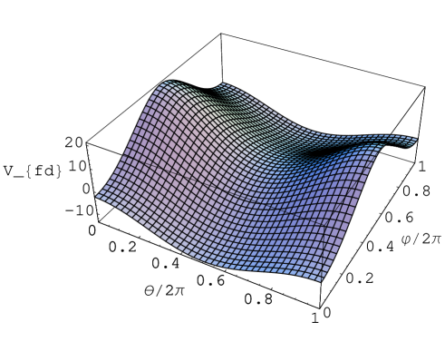
Figure 1: The behavior of ${\bar{F}}_{fd}$ for $\alpha=0,LT=1.0$. The minimum of the potential is given by $(\varphi,~{}\theta)=(0,~{}\pi)~{}({\rm mod}~{}2\pi)$.

For the adjoint fermion under the gauge group $SU(2)$, we obtain that

$${\bar{F}}_{adj} = 2\sum_{m=1}^{\infty}{1\over m^{5}}\cos(m\alpha)\bigl{(}1+\cos(2m\theta)\bigr{)}+2(LT)^{5}\Biggl{(}\sum_{l=1}^{\infty}{(-1)^{l}\over l^{5}}\bigl{(}1+\cos(2l\varphi)\bigr{)}$$ (55)

$$+\sum_{l,m=1}^{\infty}{{2(-1)^{l}}\over{[(mLT)^{2}+l^{2}]^{5/2}}}\cos(m\alpha)\biggl{(}1+\cos(2m\theta)\cos(2l\varphi)\biggr{)}\Biggr{)}.$$

From Fig.$2$, we observe that the minimum of the potential (55) is given by

$$(\varphi,~{}\theta)=\left(0,~{}{\pi\over 2}\right)~{}~{}({\rm mod}~{}\pi)$$ (56)

for $\alpha=0,LT=1.0$.

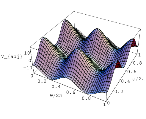
Figure 2: The behavior of ${\bar{F}}_{adj}$ for $\alpha=0,LT=1.0$. The minimum of the potential is given by $(\varphi,~{}\theta)=(0,~{}\pi/2)~{}({\rm mod}~{}\pi)$.

Let us now study the total system, that is, the fermions coupled to the gauge field. We first consider the fundamental fermion and the gauge field. The behavior of the total effective potential $N_{gauge}{\bar{F}}_{gauge}+4N_{fd}{\bar{F}}_{fd}$ is depicted in Fig.$3$, where we take $\alpha=0,LT=1.0$.

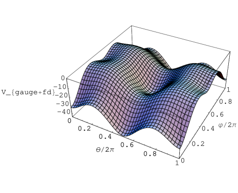
Figure 3: The behavior of $N_{gauge}{\bar{F}}_{gauge}+4N_{fd}{\bar{F}}_{fd}$ for $(N_{gauge},N_{fd})=(3,1),\alpha=0,LT=1.0$. The minimum of the potential is given by $(\varphi,~{}\theta)=(0,~{}\pi)~{}({\rm mod}~{}2\pi)$.

The minimum of the total effective potential is given by

$$(\varphi,~{}\theta)=(0,~{}\pi)~{}~{}({\rm mod}~{}2\pi).$$ (57)

$A_{k}^{(0,-1)}$ is still a massless mode for the vacuum configuration from Eq.(43), so that the $SU(2)$ gauge symmetry is not broken in this case.

The fermion contribution to the effective potential depends on the parameter $\alpha$, which twists the boundary condition for the $S^{1}$ direction (the spatial extra dimension). The physical region of $\alpha$ is given by $0\leq\alpha\leq\pi$. Since the effect of $\alpha$ shifts only the $\theta$, as seen in Eq.(44), the configuration that minimizes (53) changes according to $\alpha$. We numerically confirm that the vacuum configuration for the total potential $N_{gauge}{\bar{F}}_{gauge}+4N_{fd}{\bar{F}}_{fd}$ is given by

$$(\varphi,~{}\theta)=\left\{\begin{array}[]{lll}(0,~{}\pi)&\mbox{for}&0\leq\alpha<{\pi\over 2},\\[8.5359pt] (0,~{}0)&\mbox{for}&{\pi\over 2}\leq\alpha\leq\pi.\end{array}\right.$$ (58)

Let us note that at $\alpha_{c}\equiv\pi/2$ the fermion contribution (53) is invariant under the translation $\theta\rightarrow\theta+\pi$; that is, the periodicity with respect to $\theta$ becomes half of the original periodicity $2\pi$, so that if $\theta=0$ is the minimum configuration, so is $\theta=\pi$. The result (58) and the critical value $\alpha_{c}$ are independent of the flavor number of the fundamental fermions. The order parameter $\varphi$ does not take nontrivial values in this case. Note that, even though $\theta=\pi$, the mode $A_{k}^{(0,-1)}$ is a massless mode, so that the $SU(2)$ gauge symmetry is not broken.

Let us next consider the adjoint fermion instead of the fundamental fermion, whose contribution to the effective potential is given by Eq.(55). The behavior of the total potential $N_{gauge}{\bar{F}}_{gauge}+4N_{adj}{\bar{F}}_{adj}$ is shown in Fig.$4$ for $LT=1.0,\alpha=0$.

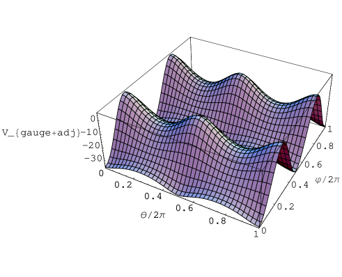
Figure 4: The behavior of $N_{gauge}{\bar{F}}_{gauge}+4N_{adj}{\bar{F}}_{adj}$ for $(N_{gauge},N_{adj})=(3,1),\alpha=0,LT=1.0$. The minimum of the potential is given by $(\varphi,~{}\theta)=(0,~{}0)~{}({\rm mod}~{}\pi)$.

The vacuum configuration is

$$(\varphi,~{}\theta)=(0,~{}0)~{}(\mbox{mod}~{}\pi).$$ (59)

The $SU(2)$ gauge symmetry is not broken in this case.

Let us consider the effect of $\alpha$ and the number of the adjoint fermions on the vacuum configuration. We numerically confirm that for $N_{adj}=1$, where $N_{adj}$ is the number of the adjoint fermions, the vacuum configuration $(\varphi,~{}\theta)=(0,~{}0)$ is independent of the values of $\alpha$. If $N_{adj}\geq 2$, we find critical values of $\alpha$, above and below which the vacuum configuration is different,

$$(\varphi,~{}\theta)=\left\{\begin{array}[]{lll}(0,~{}\pi/2)&\mbox{for}&0\leq\alpha<{\alpha_{c}},\\[8.5359pt] (0,~{}0)&\mbox{for}&\alpha_{c}<\alpha<\pi,\end{array}\right.$$ (60)

where, for example, $\alpha_{c}/2\pi\sim 0.1063,0.1623,0.1857,0.1991,0.2077$ for $N_{adj}=2,3,4,5,6$, respectively. $\varphi$ does not take nontrivial values in this case. The gauge boson becomes massive only through the nontrivial values of $\theta$, and the $SU(2)$ gauge symmetry is broken down to $U(1)$ by the Hosotani mechanism.

Let us finally consider both the adjoint and fundamental fermions. The effective potential is given by $N_{gauge}{\bar{F}}_{gauge}+4N_{fd}{\bar{F}}_{fd}+4N_{adj}{\bar{F}}_{adj}$. From the lessons obtained above, we expect that $\varphi$ does not take any nontrivial values, while $\theta$ depends on the parameter $\alpha$ and the number of flavor introduced in the theory. As an illustration, let us choose $(N_{fd},~{}N_{adj})=(1,~{}5)$ and $\alpha=0$. The behavior of the effective potential is given in Fig.$5$, where we observe that the vacuum configuration is $(\varphi,~{}\theta)=(0,~{}0.261)\times 2\pi$.

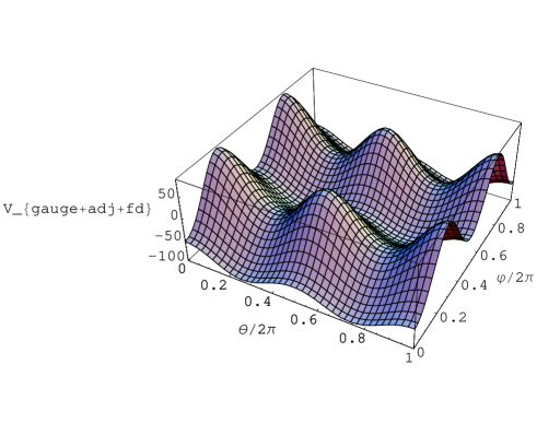
Figure 5: The behavior of $N_{gauge}{\bar{F}}_{gauge}+4N_{fd}{\bar{F}}_{fd}+4N_{adj}{\bar{F}}_{adj}$ for $(N_{gauge},N_{fd},N_{adj})=(3,1,5),\alpha=0,LT=1.0$. The minimum of the potential is given by $(\varphi,~{}\theta)=(0,~{}0.262)\times 2\pi~{}({\rm mod}~{}2\pi)$.

If we take $\alpha/2\pi=0.2$ for the same matter content, the vacuum configuration changes to $(\varphi,~{}\theta)=(0.0,~{}0.5)\times 2\pi$.

4.2 Massive matter

In this subsection we study the effect of the massive bulk fermions on the vacuum configuration. We consider the five dimensional case. By using the formula (31), the equation (48) becomes

$$L^{5}\left({3\over 4\pi^{2}}\right)^{-1}F = (-1)^{f+1}\Biggl{[}\sum_{i=1}^{N}\sum_{m=1}^{\infty}{1\over m^{5}}\left(1+mz+{m^{2}z^{2}\over 3}\right){\rm e}^{-mz}\cos[m(\theta_{i}-\alpha)]$$ (61)

$$+t^{5}\sum_{i=1}^{N}\sum_{l=1}^{\infty}{(-1)^{l}\over l^{5}}\left(1+{lz\over t}+{l^{2}z^{2}\over 3~{}t^{2}}\right){\rm e}^{-{lz/t}}\cos(l(\varphi_{i}+2\pi\eta))$$

$$+2t^{5}\sum_{i=1}^{N}\sum_{l,m=1}^{\infty}{(-1)^{l}\over{[(mt)^{2}+l^{2}]^{5/2}}}$$

$$\times\left(1+\sqrt{(mz)^{2}+(lz/t)^{2}}+{{(mz)^{2}+(lz/t)^{2}}\over 3}\right){\rm e}^{-\sqrt{(mz)^{2}+(lz/t)^{2}}}$$

$$\times\cos[m(\theta_{i}-\alpha)]\cos(l(\varphi_{i}+2\pi\eta))\Biggr{]},$$

We choose the gauge group $SU(2)$ and consider the parameter region of $t\sim z\sim 1$, which is the most interesting one because the effects of both the temperature and the scale of the extra dimension equally contribute to the effective potential. As an illustration, the behavior of the total effective potential for $(t,~{}z)=(1.1,~{}0.8),\alpha=0$ with the $SU(2)$ fundamental fermion is depicted in Fig.$6$.

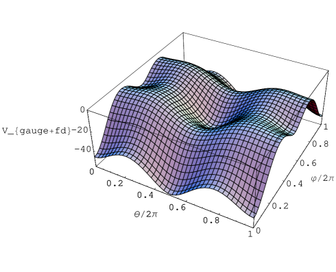
Figure 6: The behavior of $N_{gauge}{\bar{F}}_{gauge}+4N_{fd}{\bar{F}}_{fd}$ for $(N_{gauge},N_{fd})=(3,1),\alpha=0,LT=1.1,LM=0.8$. The minimum of the potential is given by $(\varphi,~{}\theta)=(0,0.5)\times 2\pi~{}({\rm mod}~{}2\pi)$

We find that the vacuum configuration is given by

$$(\varphi,~{}\theta)=(0,~{}\pi)~{}~{}({\rm mod}~{}~{}2\pi).$$ (62)

If we vary the parameter $\alpha$, the vacuum configuration changes according to the value, and we find that

$$(\varphi,~{}\theta)=\left\{\begin{array}[]{lll}(0,~{}\pi)&\mbox{for}&0\leq\alpha<{\pi\over 2},\\[8.5359pt] (0,~{}0)&\mbox{for}&{\pi\over 2}\leq\alpha\leq\pi.\end{array}\right.$$ (63)

As stated below Eq.(58), the periodicity with respect to $\theta$ for the fundamental fermion contribution becomes $\pi$ at $\alpha=\pi/2$. Again, nontrivial values of $\varphi$ are not realized and the $SU(2)$ gauge symmetry is not broken in this case.

Let us study the case of the massive adjoint fermion coupled to the gauge field. For $(t,~{}z)=(1.1,~{}0.8),\alpha=0$, we numerically find that the vacuum configuration is given by

$$\left(\varphi,~{}\theta\right)=\left(0,~{}0\right),~{}(0,~{}\pi)\quad({\rm mod}~{}~{}2\pi).$$ (64)

We next vary the parameters $\alpha$ and $N_{adj}$. The vacuum configuration $(\varphi,~{}\theta)=(0,~{}0)$ does not depend on the values of $\alpha$ for $N_{adj}=1,2$. It changes according to the values of $\alpha$ for $N_{adj}\geq 3$. For $N_{adj}=3$ we obtain that the vacuum configuration is given by

$$(\varphi,~{}\theta)=\left\{\begin{array}[]{lll}(0,~{}\pi/2)&\mbox{for}&0\leq\alpha<\alpha_{c},\\[8.5359pt] (0,~{}0)&\mbox{for}&\alpha_{c}<\alpha\leq\pi,\end{array}\right.$$ (65)

where $\alpha_{c}/2\pi\simeq 0.1336$. If we consider $N_{adj}=6$, the critical value is $\alpha_{c}/2\pi\simeq 0.1956$.

We have also numerically calculated the effective potential for the other values of $(t,~{}z)$ with $t\sim z\sim 1$. It turns out that the qualitative features are essentially the same as those for $(t,~{}z)=(1.1,~{}0.8)$.

Even if we consider the massive adjoint and fundamental fermions simultaneously, we do not have nontrivial values for $\varphi$. The VEV for $\theta$ depends on the size of the bulk mass and the flavor number introduced in the theory. The gauge boson becomes massive only through the VEV of $\theta$ and the $SU(2)$ gauge symmetry can be broken only by the Hosotani mechanism.

The boundary condition is crucial for determining the vacuum configuration of $\varphi$ and $\theta$. The boundary condition for the $S_{\tau}^{1}$ direction is uniquely fixed by the quantum statistics and nontrivial VEVs for $\varphi$ cannot be realized, as we have studied above. This is also valid for the $SU(N)$ gauge group with $N\geq 3$. On the other hand, the boundary condition for the $S^{1}$ direction is controlled by the parameter $\alpha$, on which the VEV for $\theta$ depends, in addition to the flavor number introduced into the theory.

Let us make a comment. We have studied the VEVs of $\varphi_{i}$ and $\theta_{i}$ by minimizing the effective potential. By using these values, we evaluate the second derivatives of the effective potential at the vacuum configuration ,

$${g^{2}\over T^{2}}{\partial^{2}V_{eff}\over\partial\varphi_{i}\partial\varphi_{j}}\Bigg{|}_{vac},\quad{g^{2}L^{2}}{\partial^{2}V_{eff}\over\partial\theta_{i}\partial\theta_{j}}\Bigg{|}_{vac}.$$ (66)

These give us the gauge invariant (with respect to the residual gauge symmetry) mass terms for the zero modes for $A_{\tau},A_{y}$, respectively. The mass term for the zero mode for $A_{\tau}$ is the electric mass and the one for $A_{y}$ is the scalar mass. For instance, the electric mass from the effective potential (10) and (14) for $4$ dimensions is calculated as

$$m_{ele}^{2}\equiv{g^{2}\over T^{2}}{\partial^{2}\over\partial\varphi_{i}\partial\varphi_{j}}(V_{gauge}^{T}+V_{fd}^{T})\Bigg{|}_{vac}={g^{2}\over 3}T^{2}\left(2N+N_{fd}\right)M_{ij},$$ (67)

where the vacuum configuration in this case is given by Eq.(22). Here $N_{fd}$ is the number of the massless fundamental fermions and all the (off-) diagonal elements in the $N-1$ by $N-1$ matrix $M_{ij}$ is 2 (1). If we rescale the variables $\varphi_{i}~{}(i=1,\cdots N-1),\varphi_{N}$ as $\varphi_{i}\rightarrow\varphi_{i}/\sqrt{2},\varphi_{N}\rightarrow\varphi_{N}/\sqrt{2N}$, the eigenvalue for the matrix is given by $1/2$ ($(N-1)$-degeneracy). Therefore, the electric mass is ${g^{2}\over 3}T^{2}\left(N+N_{fd}/2\right)$, which is the same result obtained in [12].

Before closing this section, it is worthwhile mentioning the high temperature behavior of the Hosotani mechanism. At high temperature, broken symmetries via the Higgs mechanism are expected to be restored because positive temperature-dependent mass squared terms are induced radiatively [10]. This is also true for the time component of the gauge field $A_{\tau}$, as shown in Eq. (67). This does not, however, hold for the extra dimensional component of the gauge field $A_{y}$. The curvature at the origin of the potential is given as

$${g^{2}L^{2}}{\partial^{2}V_{eff}\over\partial\theta_{i}\partial\theta_{j}}\Bigg{|}_{\theta=\varphi=0}.$$ (68)

To find the curvature, let us consider the effective potential (49). In the high temperature limit, the second term in Eq.(49) dominates and gives $\varphi=0$ as the vacuum configuration (we have ignored the color indices here for simplicity.). For $\varphi=0$, the third terms for the fermion ($f=1,\eta=1/2$) and for the boson ($f=0,\eta=0$) become

$$2(LT)^{D}\sum_{l=1}^{\infty}{(-1)^{l}\cos[m(\theta_{i}-\alpha)]\over[l^{2}+(mLT)^{2}]^{D/2}} = -{\cos[m(\theta_{i}-\alpha)]\over m^{D}}+(LT)^{D}\sum_{k=-\infty}^{\infty}{{2\sqrt{\pi}}\over\Gamma(D/2)}\Biggl{[}\biggl{(}{{(k+{1\over 2})\pi}\over{mLT}}\biggr{)}^{2}\Biggr{]}^{D-1\over 4}$$ (69)

$$\times\ K_{{D-1}\over 2}\Bigl{(}(2k+1)\pi mLT\Bigr{)}\cos[m(\theta_{i}-\alpha)],$$

$$-2(LT)^{D}\sum_{l=1}^{\infty}{\cos[m(\theta_{i}-\alpha)]\over[l^{2}+(mLT)^{2}]^{D/2}} = {\cos[m(\theta_{i}-\alpha)]\over m^{D}}-(LT)^{D}\Biggl{(}{{\Gamma({D-1\over 2})\sqrt{\pi}}\over\Gamma(D/2)}{1\over(mLT)^{D-1}}$$ (70)

$$+ {{2\sqrt{\pi}}\over\Gamma(D/2)}\sum_{k=-\infty,\neq 0}^{\infty}\Biggl{[}\biggl{(}{\pi k\over mLT}\biggr{)}^{2}\Biggr{]}^{D-1\over 4}K_{{D-1}\over 2}\Bigl{(}2k\pi mLT\Bigr{)}\Biggr{)}$$

$$\times\,\cos[m(\theta_{i}-\alpha)],$$

respectively. The first terms in Eqs.(69), (70) are canceled by the first term in Eq.(49). Since the modified Bessel function $K_{{D-1}\over 2}(z)$ is exponentially suppressed for large $z$, we observe from Eq.(69) that the fermions do not contribute to the dynamics of $\theta$ at high temperature.

$$F_{fermion}(\theta_{i},\varphi=0)\simeq 0.$$ (71)

Here, we have ignored the $\theta$-independent terms. On the other hand, the second term in Eq.(70) survives to control the dynamics of $\theta$. Let us note that the difference between the behavior in Eq.(69) and Eq.(70) comes from the non-existence and the existence of the zero mode in the Matsubara frequency, respectively. We obtain from Eq.(70) that the bosonic contribution to the effective potential at high temperature is given by

$$F_{boson}(\theta_{i},\varphi=0)\simeq-{T\over L^{D-1}}{\Gamma({D-1\over 2})\over\pi^{{D-1\over 2}}}\sum_{m=1}^{\infty}{1\over m^{D-1}}\cos[m(\theta_{i}-\alpha)].$$ (72)

Therefore, we have quite interesting results that there is no fermionic contribution to the curvature (68) at high temperature and that the bosonic contribution to the curvature is proportional to $T$, but the coefficients can be both positive and negative due to the boundary condition parametrized by $\alpha$ in Eq.(72). This implies that broken symmetries via the Hosotani mechanism at $T=0$ is not necessarily restored at high temperature, unlike the Higgs mechanism. Hence, we understand that, at high temperature, only the bosonic degrees of freedom determine the gauge symmetry breaking patterns, which depend on the bosonic matter contents and the boundary conditions for the $S^{1}$ direction [21].

5 Conclusions

We have studied the gauge theories with/without the extra dimension at finite temperature, and especially focused on the zero mode of the component gauge field $A_{\tau}$ for the Euclidean time direction. The zero mode is closely related with the Polyakov loop, and we have computed the effective potential for the zero mode in the one-loop approximation. We minimize the effective potential to study whether nontrivial values for $\langle A_{\tau}\rangle$ are realized or not.

The vacuum structure crucially depends on the boundary conditions of the fields for the compactified direction. In the present case, the boundary condition of the field for the Euclidean time direction is uniquely fixed by the quantum statistics. This is a big difference from the case of the boundary condition of the field for the spatial compact extra dimension. In the pure $SU(N)$ gauge theory and the $SU(N)$ gauge theory with the massless adjoint matter, the Polyakov loop takes the values at the center of the $SU(N)$, and this is consistent with the lattice result in the high temperature region for $SU(3)$. For the fundamental massless matter coupled to the gauge field, no nontrivial values for $\langle A_{\tau}\rangle$ are induced, so that the gauge symmetry is not broken and the gauge bosons remain massless. The boundary condition for the Euclidean time direction prevents $\langle A_{\tau}\rangle$ from taking nontrivial values.

We have also considered the massive bulk matter to see the effect of the bulk mass on $\langle A_{\tau}\rangle$. The matter with $M/T\gg 1$ decouples from the effective potential due to the Boltzmann factor. Although a small bulk mass tends to induce nontrivial VEVs, the effect is too small to realize the gauge symmetry breaking.

In order to investigate further the possibility of having nontrivial VEVs for $A_{\tau}$, we have considered one spatial extra dimension at finite temperature, which is compactified on $S^{1}$, and have studied the gauge theories on $S^{1}_{\tau}\times R^{3}\times S^{1}$. There are two kinds of the order parameters in this case, that is, $\theta_{i}$ and $\varphi_{i}$, as given in Eq.(42). The Wilson loop and the Polyakov loop are the relevant quantities for the dynamics. We have computed the effective potential for the order parameters along the flat direction (41) and minimize it to determine the vacuum configuration. The boundary conditions for the $S^{1}$ direction is parametrized by $\alpha$, and those for the $S_{\tau}^{1}$ direction is uniquely fixed by the quantum statistics. The effective potential (44) is regarded as a special case of the six dimensional gauge theory compactified on $T^{2}$ with appropriate boundary conditions. As far as our numerical analyses are concerned, no nontrivial values for $\langle A_{\tau}\rangle$ are realized and the gauge symmetry breaking can occur only through nontrivial values for $\theta_{i}$.

In our analyses, the gauge bosons become massive only through $\theta_{i}$; that is, the gauge symmetry is broken by the Hosotani mechanism. We do not find the models in which the gauge symmetry is broken through the VEV of $A_{\tau}$. No nontrivial values of $\langle A_{\tau}\rangle$ are obtained. As long as the boundary condition for the Euclidean time direction is fixed by the quantum statistics, our analyses strongly suggest that it is impossible to break dynamically the gauge symmetry through $\langle A_{\tau}\rangle$ in perturbation theory. It may be challenging to find models in which the Polyakov loop $W_{p}$ in Eq.(12) takes nontrivial values nonperturbatively.

Acknowledgments

This work is supported in part by a Grant-in-Aid for Scientific Research (No. 18540275) from the Japanese Ministry of Education, Science, Sports and Culture. The authors would like to thank Professors T. Onogi(Yukawa Inst.), H. So(Ehime Univ.) and H. Yoneyama(Saga Univ.) for valuable discussions and K.T. is also supported by the 21st Century COE Program at Tohoku University.

References

- [1] M. Sakamoto, M. Tachibana and K. Takenaga, Phys. Lett. B457 (1999) 33, Phys. Lett. B458 (1999) 231, Prog. Theor. Phys. 104 (2000) 633.
- [2] H. Hatanaka, K. Ohnishi, M. Sakamoto and K. Takenaga, Prog. Theor. Phys. 107 (2002) 1191, Prog. Theor. Phys. 110 (2003) 791.
- [3] K. Ohnishi and M. Sakamoto, Phys. Lett. B486 (2000) 179, H. Hatanaka, S. Matsumoto, K. Ohnishi and M. Sakamoto, Phys. Rev. D63 105003 (2001).
- [4] Y. Hosotani, Phys. Lett. B126 (1983) 309, Ann. Phys. (N.Y.) 190, 233 (1989).
- [5] A. T. Davies and A. McLachlan, Nucl. Phys. B317 237 (1989), A. McLachlan, Nucl. Phys. B338 188 (1990), J. E. Hetrick and C. L. Ho, Phys. Rev. D40 (1989) 4085, C. L. Ho and Y. Hosotani, Nucl. Phys. B345 445 (1990), A. McLachlan, Nucl. Phys. B338 188 (1990), H. Hatanaka, Prog. Theor. Phys. 102 (1999) 407.
- [6] K. Takenaga, Phys. Lett. B425 (1998) 114, Phys. Rev. D58 (1998) 026004, Phys. Rev. D66 085009 (2002), Phys. Lett. B570 (2003) 244, N. Haba, K. Takenaga and T. Yamashita, Phys. Lett. B605 (2005) 355.
- [7] N. V. Krasnikov, Phys. Lett. B273 (1991) 246, H. Hatanaka, T. Inami and C.S. Lim, Mod. Phys. Lett. A13 (1998) 2601, G. R. Dvali, S. Randjbar-Daemi and R. Tabbash, Phys. Rev. D65 064021 (2002), N. Arkani-Hamed, A. G. Cohen and H. Georgi, Phys. Lett. B513 (2001) 232, I. Antiniadis, K. Benakli and M. Quiros, New J. Phys. 3, (2001),20.
- [8] C. Csaki, C. Grojean, H. Murayama, Phys. Rev. D67 085012 (2003), C. Csaki, C. Grojean, H. Murayama, L. Pilo and J. Terning, Phys. Rev. D69 055006 (2004), K. Choi, N. Haba, K. S. Jeong, K. Okumura, Y. Shimizu and M. Yamaguchi, JHEP 02 (2004) 037, Y. Hosotani, S. Noda and K. Takenaga, Phys. Rev. D69 125014 (2004), Phys. Lett. B607 (2005) 276, N. Haba, K. Takenaga and T. Yamashita, Phys. Rev. D71 025006 (2005), G. Panico, M. Serone and A. Wulzer, Nucl. Phys. B739 (2006) 186, G. Panico and M. Serone, JHEP 05 (2005) 024, N. Maru and K. Takenaga, Phys. Rev. D72 046003 (2005), Phys. Rev. D74 015017 (2006).
- [9] R. Contino, Y. Nomura and A. Pomarol, Nucl. Phys. B671 (2003) 148, K. Oda and A. Weiler, Phys. Lett. B606 (2005) 408, K. Agashe, R. Contino and A. Pomarol, Nucl. Phys. B719 (2005) 165, Y. Hosotani and M. Mabe, Phys. Lett. B615 (2005) 257, Y. Hosotani, S. Noda, Y. Sakamura and S. Shimasaki, Phys. Rev. D73 096006 (2006), Y. Sakamura and Y. Hosotani, Phys. Lett. B645 (2007) 442, hep-ph/0703212.
- [10] L. Dolan and R. Jackiw, Phys. Rev. D9 (1974) 3320, S. Weinberg, Phys. Rev. D9 (1974) 3357.
- [11] H. Hata and T. Kugo, Phys. Rev. D21 (1980) 3333.
- [12] D. Gross, R. Pisarski and L. Yaffe, Rev. Mod. Phys. 53 (1981) 43.
- [13] N. Weiss, Phys. Rev. D24 (1981) 475; Phys. Rev. D25 (1982) 2667.
- [14] C. P. Korthals and M. Laine, Phys. Lett. B511 (2001) 269.
- [15] K. Farakos and P. Pasipoularides, Nucl. Phys. B705 (2005) 92.
- [16] M. Quiros, For a review, see, for example, hep-ph/0302189.
- [17] A. Masiero, C. A. Scrucca, M. Serone and L. Silvestrini, Phys. Rev. Lett. 87 251601 (2001).
- [18] Y. Iwasaki, et.al., Phys. Rev. D46 (1992) 4657.
- [19] A. T. Davies and A. McLachlan, Phys. Lett. B200 (1988) 305, K. Takenaga, Phys. Rev. D64 066001 (2001),
- [20] N. Haba, S. Matsumoto, N. Okada and T. Yamashita, JHEP 0602 (2006) 073, N. Maru and K. Takenaga, Phys. Lett. B637 (2006) 287.
- [21] For details, M. Sakamoto and K. Takenaga, in preparation.