A Bayesian approach to strong lensing modelling of galaxy clusters

Abstract

In this paper, we describe a procedure for modelling strong lensing galaxy clusters with parametric methods, and to rank models quantitatively using the Bayesian evidence. We use a publicly-available Markov Chain Monte-Carlo (MCMC) sampler (“BayeSys”), allowing us to avoid local minima in the likelihood functions.

To illustrate the power of the MCMC technique, we simulate three clusters of galaxies, each composed of a cluster-scale halo and a set of perturbing galaxy-scale subhalos. We ray-trace three light beams through each model to produce a catalogue of multiple images, and then use the MCMC sampler to recover the model parameters in the three different lensing configurations.

We find that, for typical HST-quality imaging data, the total mass in the Einstein radius is recovered with $\sim$ 1% to 5% error according to the considered lensing configuration. However, we find that the mass of the galaxies is strongly degenerate with the cluster mass when no multiple images appear in the cluster centre. The mass of the galaxies is generally recovered with a 20% error, due largely to the poorly constrained cut-off radius.

Finally, we describe how to rank models quantitatively using the Bayesian evidence. We confirm the ability of strong lensing to constrain the mass profile in the central region of galaxy clusters in this way. Ultimately, such a method applied to strong lensing clusters with a very large number of multiple images may provide unique geometrical constraints on cosmology.

The implementation of the MCMC sampler used in this paper has been done within the framework of the lenstool software package, which is publicly available.

1 Introduction

Strong gravitational lensing is produced when a distant object (such as a galaxy or a quasar) is serendipitously aligned with a critical foreground mass concentration. Such a phenomenon was first observed by Walsh et al. (1979) who discovered a double quasar strongly lensed by a distant galaxy. In the 1980’s, with the advent of CCD imaging and its application to astronomy, giant gravitational arcs in galaxy cluster cores were discovered by two independent teams (Lynds and Petrosian 1986; Soucail et al. 1987). The lensing explanation proposed by Paczynski (1987) was soon confirmed by Soucail et al. (1988), who measured the redshift for the giant arc in Abell 370 as being roughly twice that of the cluster redshift. Together with the multiply-imaged quasars, giant arcs in galaxy clusters turned strong gravitational lensing from a theoretical curiosity into a powerful tool to probe the mass distributions of galaxies and galaxy cluster cores. Although rare in current surveys, strong lensing events are expected to number as many as a few hundred thousand over the whole sky (Cabanac et al. 2007).

In order to fully exploit strong gravitational lensing events, one generally needs high resolution imaging coupled to deep spectroscopy to measure the redshift of both the lensing object and the lensed sources. By combining, Hubble Space Telescope (HST) images with ground-based spectroscopy on 8-10m telescopes, strong lensing analysis has proved to be very successful at constraining the mass distribution of galaxies (e.g.  Muñoz et al. 1998; Koopmans et al. 2006) and galaxy cluster cores (e.g.  Kneib et al. 1996; Abdelsalam et al. 1998; Smith et al. 2005; Halkola et al. 2006).

Nowadays, one particularly interesting application of strong lensing is to constrain the dark matter (DM) distribution in cluster cores, and contrast it with predictions of numerical simulations. For example, we would like to measure accurately the inner slope and the concentration parameter of the DM density profile, to probe DM properties and its link with the baryonic component (Sand et al. 2007, and references therein). Indeed, numerical simulations seem to advocate a cuspy DM slope that could be described by an NFW (Navarro et al. 1997) or a Sérsic (Sérsic 1968; Merritt et al. 2005) profile. Observations are not yet giving definitive answers relative to the value of the inner slope (Gavazzi et al. 2003; Sand et al. 2004, 2007) or the concentration (Kneib et al. 2003; Gavazzi et al. 2003), but progress is being made steadily.

For example, in Abell 1689, after much disagreement over its concentration (Clowe and Schneider 2001; King et al. 2002; Bardeau et al. 2005; Broadhurst et al. 2005; Halkola et al. 2006), Limousin et al. (2007) came to a consensus value of $c_{vir}\sim 6-8$ after careful and detailed modelling of the previously-analysed data combined with new multiple image identifications, redshifts and weak lensing source galaxy colours. Comerford and Natarajan (2007) discuss the issues related to the determination of the concentration parameter with different techniques, and compare its measurement in a large compilation of galaxy clusters with the distribution of $c_{vir}$ in numerical simulations.

Numerical studies have shown that the concentration parameter of the NFW potential is quite sensitive to complex structures along the line of sight (King and Corless 2007) or triaxiality of the dark matter halos (Corless and King 2006). Improved datasets, but also more advanced techniques are needed to accurately model the mass distribution of gravitational lenses such as these. This movement towards more complex models has generated two competitive methodologies for lens modelling.

So-called “non-parametric” methods, where the mass distribution or lens potential is reconstructed as a map defined on a grid of pixels, have been developed to constrain the mass distribution of (admittedly well-constrained) galaxy-scale lenses (Saha and Williams 1997; Abdelsalam et al. 1998), initially for the purpose of probing the large diversity of possible mass models with a view to investigating in particular the modelling degeneracy present in the measurement of the Hubble constant. Since 1997, non-parametric modelling has been intensively tested and greatly improved to overcome the lack of constraints very common in strong lensing (e.g.  Koopmans 2005; Diego et al. 2005; Kochanek 2006). However, the flexibility of these methods arising from their very large number of parameters has to be controlled to avoid over-fitting the data. Recent work on regularisation techniques Bradač et al. (2005); Suyu et al. (2006) has improved the situation in this regard somewhat. However, physical understanding often comes from the measurement of quantities such as total mass, profile slope, and so on, which still have to be extracted from the flexible reconstructed maps.

“Parametric”, or rather, simply-parameterised models therefore have two advantages: the assumption of a physical model leads to inferences that are directly related to physical quantities, while the model fits the data with relatively few free parameters compared to a “non-parametric” model.

Effectively the regularisation of the mass distribution is achieved through the physical model itself. The predicted surface density maps are smooth (by design), a situation perhaps valid only for quiet systems where the galaxy dynamics are well understood. The modelling of merging and perturbed systems is clearly the next challenging step for parametric methods.

Another important issue in both parametric and non-parametric methods is the way the parameter space is explored. In this paper, we have used the parametric gravitational lensing package lenstool to perform the lens modelling. Given a parametrization describing the lens, this software explores the parameter space around the best-fit region, reproducing the location of the observed multiple images within the supplied uncertainties. The first versions of the software (Kneib et al. 1993; Smith et al. 2005) were based on a downhill $\chi^{2}$ minimization. However, this technique is very sensitive to local minima in the likelihood distribution; as a result, the modelling of complex systems would rapidly become too involving and inefficient.

In order to face the current and future observational data, we have thus implemented a new optimization method based on a Bayesian Markov Chain Monte Carlo (MCMC) approach. We will investigate here the merits of this new method on simulated strong lensing clusters.

In the first part of the paper, we explain how to model a cluster of galaxies, and how to identify systems of multiple images. Then, we describe the implementation of the MCMC package bayesys (Skilling 2004) in the lenstool software. In the second part, we analyse the performance of the Bayesian MCMC sampler by studying the degeneracies between the parameters of the Peudo-Isothermal Elliptical Mass Distribution (PIEMD, Kassiola and Kovner 1993), the pseudo-elliptical Navarro, Frenk & White (NFW, e.g.  Navarro et al. 1997; Golse et al. 2002) and the pseudo-elliptical Sérsic potentials. In the last section, we use the Bayesian evidence to rank the models that best reproduce systems of multiple images simulated from galaxy clusters with flat inner mass profiles. Finally, we discuss the limitations of the strong lensing modelling.

Note that the lenstool Bayesian MCMC implementation has already been used to model Abell 1689 (Limousin et al. 2007), Abell 68 (Richard et al. 2007), MS 2053 (Verdugo et al. 2007) and Abell 2390 (Jullo et al. 2007). All our results are scaled to the flat, low matter density $\Lambda$cdm cosmology with $\Omega_{\rm{M}}=0.3,\ \Omega_{\Lambda}=0.7$. When necessary, we scale the masses and distances according to a Hubble constant of H${}_{0}=70$ km s^-1 Mpc^-1.

2 Definitions and Methodology

2.1 Definition

The gravitational lensing transformation is a mapping from the source plane to the image plane (Schneider et al. 1992):

$$\beta=\theta-\nabla\varphi(\theta)\;,$$ (1)

where $\theta$ and $\beta$ are the image and source positions respectively and $\varphi(\theta)$ is the lens potential computed at the image position. Depending on the strength of the gradient of the lens potential, one can easily see that for a given source position $\beta$, multiple images (at different $\theta$) can solve the lensing equation. When this is happening it corresponds to the strong lensing regime.

The lens potential is the product of angular diameter distances ratio: $D_{LS}/D_{OS}$ (Lens-Source distance over Observer-Source distance) and the projected Newtonian potential $\phi(\theta)$ at the image position:

$$\varphi(\theta)={2\over c^{2}}{D_{LS}\over D_{OS}}\phi(\theta)\;.$$ (2)

Hence, once the distance of the lens and the source are known, solving the lensing equation for different multiple images, allows to directly constrain the Newtonian potential, or equivalently the mass distribution of the lens.

2.2 Modelling the different cluster mass components

Observations of clusters of galaxies reveal two components: cluster-scale halos (which includes both DM and the baryonic intra cluster gas) and galaxy-scale halos (made of stars and DM). Similarly, N-body simulations of clusters show that the mass distribution of subhalos inside a cluster halo follows a Schechter function (e.g.  Shaw et al. 2006).

Thus, cluster gravitational potential can be decomposed in the following manner:

$$\phi_{tot}=\sum_{i}\phi_{c_{i}}+\sum_{j}\phi_{p_{j}}\;,$$ (3)

where we distinguish the cluster-scale smooth and large potentials $\phi_{c_{i}}$, and the subhalo potentials $\phi_{p_{j}}$ providing small perturbations (Natarajan and Kneib 1997). In the following, we consider a subhalo as a clump of matter containing a galaxy: we assume that there are no dark galaxies in clusters. This decomposition has been successful in reproducing the observed systems of multiple images and in constraining the size of the subhalos in clusters (e.g.  Smith et al. 2005; Natarajan et al. 2006). We now describe in more detail how we model the cluster-scale halos and galaxy-scale subhalos.

2.2.1 Smooth cluster-scale halos

The smooth cluster-scale halos represent both the DM and the intra-cluster gas. With enough constraints, each of these two component could in principle be modelled separately, but in this work they are modelled together as a single mass component. The number of such halos is not easy to evaluate; generally one starts with a single halo – except when X-Ray observations or the distribution of the galaxies clearly show a multi-modal distribution – and increases the complexity of the model from there.

In the case of a multi-modal distribution or a clearly bad fit to the data with a single halo, additional halos can be included to the model until a good fit is reached. In the lenstool literature to date no more than two cluster-scale halos have been needed to achieve a good model (e.g. Abell 2218, Abell 1689), but this may change in the near future with the expected improvement of the strong lensing data (in particular with more spectroscopic redshifts) or when properly taking into account external constraints.

Each halo in a model (both the cluster-scale and the galaxy-scale described below) is parametrized by a position on the sky ($x_{c},y_{c}$), a projected ellipticity of the mass distribution ($\epsilon_{\Sigma}$) (see also  B for the pseudo-elliptical developments of the Sérsic potential), a position angle (PA), and a set of parameters specific to the choice of potential profile used to describe the halo. In this paper, we consider either the SIE, NFW, PIEMD, or Sérsic profiles, described by either 1, 2, 3, or 3 parameters respectively (see Table 1 for the analytic description of each potential. See also Limousin et al. (2005) for the surface density definitions of the PIEMD and NFW potentials).

Table 1: lenstool most used potentials.

• SIE
  $\epsilon_{\varphi}$	=	$\epsilon_{\Sigma}/3$	$(\epsilon_{\Sigma}<0.4)^{a}$
  $\rho$	=	$\rho_{0}/\tilde{R}$
  $\rho_{0}$	=	$\displaystyle\frac{\sigma^{2}}{2\pi G}$
  PIEMD
  $\epsilon_{\varphi}$	=	$\displaystyle\frac{1-\sqrt{1-\epsilon_{\Sigma}^{2}}}{\epsilon_{\Sigma}}$
  $\rho$	=	$\displaystyle\frac{\rho_{0}}{(1+\frac{\tilde{R}^{2}}{r_{c}^{2}})(1+\frac{\tilde{R}^{2}}{r_{cut}^{2}})}$
  $\rho_{0}$	=	$\displaystyle\frac{\sigma_{\infty}^{2}}{2\pi Gr_{c}^{2}}$	$(\sigma_{0}\simeq\sigma_{\infty}/1.46)^{b}$
  NFW
  $\epsilon_{\varphi}$	=	$\epsilon_{\Sigma}/2.27$	$(\epsilon_{\varphi}<0.25)^{c}$
  $\rho$	=	$\displaystyle\frac{\delta_{c}\rho_{c}}{\frac{\tilde{R}}{r_{s}}(1+\frac{\tilde{R}}{r_{s}})^{2}}$
  $\delta_{c}$	=	$\frac{200}{3}\frac{c^{3}}{\ln(1+c)-c/(1+c)}$	$r_{s}=\frac{r_{vir}}{c}$
  Sérsic
  $\epsilon_{\varphi}$	=	$\epsilon_{\Sigma}/3.55$	$(\epsilon_{\varphi}<0.25)$
  $\ln\left(\frac{\Sigma}{\Sigma_{e}}\right)$	=	$-b_{n}\left[\left(\frac{\tilde{R}}{R_{e}}\right)^{\frac{1}{n}}-1\right]$
  $b_{n}$	$\simeq$	$2n-\frac{1}{3}+\frac{4}{405n}+\frac{46}{25515n^{2}}^{d}$
  a Kneib et al. (1993)
  b Golse (2002)
  c Golse and Kneib (2002)
  d Ciotti and Bertin (1999)

In Figure 1, we compare the surface density of the SIS, the Sérsic, the NFW and the PIEMD profiles both in the very central and in the very outer regions. These regions are accessible either to strong or weak lensing. These profiles are the best fit to the set of plotted multiple images. We clearly note the flat core of the PIEMD profile up to 10 kpc and in contrast the monotonically increasing slope of the NFW and the Sérsic profiles. The SIS profile slope is constant and hardly follows the other profiles.

• 

Figure 1: Surface density comparison between the Sérsic (solid line), the NFW (dashed line), the PIEMD (dotted line) and the SIS profiles (dot-dashed line) The surface densities correspond to the fit performed in section 5 and extended to very small and large radii. The arrows mark the multiple images positions used as constraints.

Given the data (e.g. strong lensing or dynamics data), the cluster brightest galaxy – also called the cD galaxy in the following – can either be included in the cluster-scale halo or modelled separately. However, Smith et al. (2005) showed that the centre of mass of the cluster-scale halo can be different from the cD galaxy centre. Therefore, it is generally justified to model the cD galaxy as an additional subhalo.

2.2.2 Galaxy-scale components

Kneib et al. (1996) first demonstrated that the inclusion of galaxy-scale subhalos was necessary to reproduce the observed systems of multiple images, particularly those appearing near cluster galaxies. These galaxy-scale subhalos or perturbers can be probed in a direct way using weak galaxy-galaxy lensing techniques (Natarajan and Kneib 1997; Natarajan et al. 2002), however in this paper we will concentrate only on the strong lensing aspects.

The number of subhalos to include in a model needs to be quantified. To date, a conservative attitude has been adopted: all the massive cluster member galaxies with cluster-centric radii out to approximately two times the limits of the strong lensing region are included. This is generally achieved by selecting galaxies within the cluster red sequence and selecting them brighter than a given luminosity limit. Moreover, the subhalos shape (ellipticity and orientation) is usually taken to be the same as its galaxy .

Recently, Wambsganss et al. (2005) and King and Corless (2007) have raised the issue of multiple halos/subhalos along the line of sight that increase the projected surface density and thus affect the lensing strength. While not large, this effect is a systematic, and so lensing models must consider the possibility of such gravitational perturbations. In practice, the mass distribution along the line of sight can be understood from spectroscopic and photometric measurements in the field of view.

Here, we propose a set of criteria for including perturbing subhalos in a model. The basic idea is to measure their strong lensing deviation angle and compare it to the spatial resolution $\delta$ of the lensing observations ($\delta\sim 0.1^{\prime\prime}$ for HST). A subhalo is included in the model if it can increase significantly the deflection angle at its associated galaxy position. For a cluster member galaxy if its Einstein radius $R_{Einstein}>\delta/\mu$ (where $\mu$ is the magnification of the cluster-scale halo at the position of the galaxy) then it is included, otherwise its lensing contribution is not important and it is disregarded. For galaxies not part of the cluster, if $R_{Einstein}>\delta/\mu$ and the associated galaxy is in projection out of the strong lensing region, we include it in the model at the cluster redshift by rescaling its mass so that the global lensing effect is preserved. Finally, if the galaxy is in the strong lensing region and its lensing effect is detectable then the associated subhalo must be included with a proper multi-plane lensing technique (we will not discuss such a case here as it is beyond the scope of this paper).

Accounting for all the subhalos in a galaxy cluster as individually optimisable potentials would lead to an under-constrained problem. Assumptions must be made in order to make the number of parameters commensurate with the number of constraints. Koopmans et al. (2006) have shown that a strong correlation exists between the light and the mass profiles of elliptical galaxies in the field. Consequently, in a first approximation, the subhalos position, ellipticity and orientation are matched to their luminous counterpart.

As we will show in the second part of this paper, apart from a few subhalos perturbing multiple images close to them, the vast majority of subhalos act merely to increase the total mass enclosed in the Einstein radius. Strong lensing provides few constraints on the mass profile parameters of most individual subhalos.

We therefore reduce the number of subhalo parameters by asserting exact scaling relations between the subhalo masses and their associated galaxy luminosities. Following the work of Brainerd et al. (1996), we model cluster subhalos with PIEMD potentials. The mass profile parameters in this model are the core radius ($r_{core}$), cut-off radius ($r_{cut}$), and velocity dispersion ($\sigma_{0}$), which we take to scale with the galaxy luminosity $L$ in the following way:

$$\left\{\begin{array}[]{l}\sigma_{0}=\sigma_{0}^{\star}(\frac{L}{L^{\star}})^{1/4}\;,\\ r_{core}=r_{core}^{\star}(\frac{L}{L^{\star}})^{1/2}\;,\\ r_{cut}=r_{cut}^{\star}(\frac{L}{L^{\star}})^{\alpha}\;.\\ \end{array}\right.$$ (4)

The total mass of a subhalo scales then as:

$$M=(\pi/G)(\sigma_{0}^{\star})^{2}r_{cut}^{\star}(L/L^{\star})^{1/2+\alpha}\;,$$ (5)

where $L^{\star}$ is the typical luminosity of a galaxy at the cluster redshift, and $r_{cut}^{\star}$, $r_{core}^{\star}$ and $\sigma_{0}^{\star}$ are its PIEMD parameters. When $r_{core}^{\star}$ vanishes, the potential becomes a singular isothermal potential truncated at the cut-off radius. This is generally the type of potential used in weak galaxy-galaxy lensing studies to measure the tidal radius of galaxy-scale subhalos in clusters or in the field (see Limousin et al. (2005, 2006)).

In these scaling relations, the velocity dispersion scales with the total luminosity in agreement with the Tully-Fisher and the Faber-Jackson relations for spiral and elliptical galaxies respectively. The $r_{cut}$ relation is more hypothetical. If $\alpha=0.5$, it assumes a constant mass-to-light ratio independent of the galaxy luminosity. If $\alpha=0.8$, the mass-to-light ratio scales with $L^{0.3}$ similar to the scaling of the fundamental plane (Natarajan and Kneib 1997; Jørgensen et al. 1996; Halkola et al. 2006).

2.3 Constraints

2.3.1 Multiple images

In the strong lensing regime, the light coming from a background galaxy (the source) passes through a high density region and is lensed into multiple images. The position, shape and flux of each multiple image depends on the properties of the lens and the redshift of the source. The precise measurement of the source redshift, and of the image properties (such as position, ellipticity and orientation) provides strong constraints on the lens model.

In general, image properties can be inferred from their light distributions. Indeed, the first order moment provides the image position, and the PSF-corrected second order moment gives the ellipticity and the position angle of the image. Note however, that the ellipticity of a curved arc is somewhat ill-defined, so this information can only be used if the images are relatively compact. In this paper, we only consider the multiple image’s position as a constraint, and we discuss the associated likelihood in the next section.

Sometimes, the background galaxy presents several bright regions that can be individually identified in each multiple image. Matching these bright regions in each image brings even tighter constraints to the lensing model.

The images flux can also be considered as a constraint. However, the amplification can vary strongly across highly extended images, and properly computing the amplification to measure the total flux in each image is usually not straightforward.

Finally, the redshift of the source is a strong constraint on the lens model. A spectroscopic determination is best, but a photometric redshift (e.g. Ilbert et al. (2006)) can be sufficient if accurate enough (e.g. $\sigma_{z}<0.05$ introduces a 2% error on the $D_{LS}/D_{OS}$ ratio for a lens and a source at redshifts $z_{L}=0.2$ and $z_{S}=1$ respectively) and with no multiple peak in its probability distribution (no catastrophic redshift).

For well-defined photometric redshifts, lenstool provides a way of introducing accurately the redshift likelihood as a prior for the model.

Including an uncertain source redshift as a free parameter to be inferred from the data gives the model more freedom, albeit at some extra computational cost. However, due to the other available constraints, it may lead to a more accurate redshift for that image system. This procedure may also raise questions about a photometric or spectroscopic measured redshift if the model favours a different range of values.

The correct identification of multiple images is probably the most complex task in strong lensing modelling.

Initially we consider (as a guide) only generic geometrical lensing configurations – cusp, fold and saddle (Blandford and Narayan 1986) – for single cluster-scale halo. Having found a basic model that satisfies the most obvious or most straightforward multiple image system, the perturbations due to galaxy-scale subhalos can be taken into account. Generally, subhalos do not create strong lensing events by themselves, but affect the multiple images produced by the cluster-scale halo. They can deflect their position or occasionally further divide a multiple image.

Comparing the colours of multiple images is another straightforward technique. As lensing is achromatic, multiple images must have similar colours unless the images’ fluxes are strongly contaminated with or reddened by nearby galaxies.

It is important to realize that the identification process of multiple images is both iterative and strongly linked to the determination of the mass profile, starting from the most obvious systems close to the cluster centre and progressively adding perturbations and new systems. New multiple images can be predicted before they are observationally confirmed.

2.3.2 Other lensing constraints

Single images

Single images with known redshift lying close to the strong lensing region (typically when $R_{Einstein}<r<2R_{Einstein}$) can also be included in the lens model. Indeed, they can help in constraining the parts of the model where no multiple image system is detected. Such constraints have been neglected up to now. We propose here an efficient way to include them in the $\chi^{2}$ determination.

In essence, we add a penalizing term to the likelihood if an observed single image is predicted to be multiple, and if at least one of the counter-images could effectively be detected in the observed data image. The penalizing term is a function of $n_{k}$, the number of predicted images above the detection limit (defined to be 3 times the sky noise flux in the object detection aperture).

The penalizing term is implemented in the following way:

$$\chi_{single}^{2}=\sum_{j=1}^{n_{k}}\frac{[x_{single}-x^{j}(\boldsymbol{\theta})]^{2}}{\sigma_{single}^{2}}.$$ (6)

Here, $x_{single}$ is the position of the observed single image and $x^{j}(\boldsymbol{\theta})$ is the position of a detectable image predicted by the current model, whose parameters are $\boldsymbol{\theta}$ and $\sigma_{single}$ is the position error of the observed single image.

This implementation provides a smooth way of converging to the best $\chi_{single}^{2}$. Once $\chi_{single}^{2}=0$ (as it must be if truly single), the single image is no more a constraint. Consequently, this definition only imposes an upper limit on the enclosed mass at the single image position. The truly singly-imaged systems do not add to the overall number of degrees of freedom, nor to the final global chi-squared value. However, they do accelerate the convergence on the best fitting parameter region.

This penalizing term must be used with some care; in particular, instances where $\chi_{single}^{2}>0$ have to be flagged and investigated, as they indicate either a failure of the model or that the single image identification was incorrect. Indeed, this is one way in which new multiple images may be found.

Location of critical lines

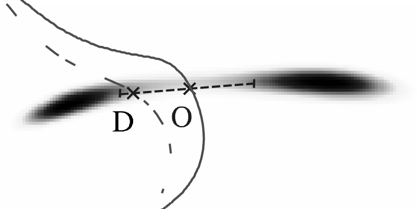
In the case of fold images, the position of the critical line passing in between the 2 images can sometimes be observed as a saddle point in the surface brightness of the images. We can use this information to put a constraint on the lens model by minimizing the distance between the position where the image isophotes cross and the critical line predicted by a model, as shown in Fig. 2.

Figure 2: Merging of two multiple images and determination of the distance between the true critical line (solid line, showing the surface brightness saddle point) and a predicted critical line (dashed line). The dashed segment represents the prior that would be set on the critical line location.

The prior segment for the critical line position can be defined by a centroid $\mathbf{O}$, a position angle and a Gaussian error size on the position $\sigma_{cl}$, hence, the corresponding $\chi^{2}$ can be given as:

$$\chi^{2}_{cl}=\frac{||\mathbf{O}-\mathbf{D}||^{2}}{\sigma_{cl}^{2}}\;,$$ (7)

where $\mathbf{D}$ is the intersection of the predicted critical line and the defined prior segment.

This constraint merely reinforces the weight of the considered system of multiple images in the model.

By focusing on the crossing isophote, it makes of use of more of the imaging information than just the centroids of the multiple images. As such, it is a low-cost constraint in terms of computation time and definitely accelerates the convergence on the best fit region. Of course, since constraints must be independent observations, this constraint must be observable and not computed from the image positions.

At the end of the optimisation, we check that $\chi^{2}_{cl}<1$. If this is not satisfied, then either the critical constraint was wrongly identified or the model has not yet fully converged.

Weak shear signal

Outside the strong lensing region, the weak shear signal can be used to constrain the model on larger angular scales. Considering a catalogue of background galaxies with PSF-corrected shape measurements, one can minimize the difference between the ellipticity of each galaxy and the reduced shear predicted by a mock model at the galaxy location (see e.g.  Marshall et al. 2002, and references therein). We will discuss the weak lensing implementation in a forthcoming paper

2.4 The multiple images’ likelihood

We assume that the noises associated with the measurement of the images position are Gaussian and uncorrelated from one image to another. The noise covariance matrix for all the considered systems of multiple images is therefore diagonal. Hence, the usual definition of the likelihood function applies and becomes, in this case,

$$\mathcal{L}=\mathrm{Pr}(D|x(\boldsymbol{\theta}))=\prod_{i=1}^{N}\frac{1}{\prod_{j}\sigma_{ij}\sqrt{2\pi}}\exp^{-\frac{\chi^{2}_{i}}{2}}\;,$$ (8)

where $N$ is the number of sources, and $n_{i}$ is the number of multiple images for source $i$. The contribution to the overall $\chi^{2}$ from multiple image system $i$ is

$$\chi^{2}_{i}=\sum_{j=1}^{n_{i}}\frac{[x^{j}_{\mathrm{obs}}-x^{j}(\boldsymbol{\theta})]^{2}}{\sigma_{ij}^{2}}\;,$$ (9)

where $x^{j}(\boldsymbol{\theta})$ is the position of image $j$ predicted by the current model, whose parameters are $\boldsymbol{\theta}$ and $\sigma_{ij}$ is the error on the position of image $j$.

The accurate determination of $\sigma_{ij}$ depends on the image S/N ratio. For extended images, a pixellated approach is the only accurate method which takes the S/N ratio of each pixel into account (Dye and Warren 2005; Suyu et al. 2006). However, this method is very time consuming. Therefore, in a first approximation, the image position error can be determined by fitting a 2D Gaussian profile to the image surface brightness. In this case, the fit error contains implicitly the S/N ratio of each pixel. However, this assumes that the background galaxy is compact and its surface brightness profile is smooth so that the brightest point in the source plane match the brightest point in the image plane. In this paper, for simplicity, the image positions are determined by inverting the lens equation for a given source position. Therefore, the images are point-like. We assign them identical $\sigma_{ij}$ so that they have the same weight in the likelihood computation. Of course, this procedure is valid only in simulations where the source positions are known a priori and could not be applied to real cases.

A major issue of the $\chi^{2}$ computation is of how to match the predicted and observed images one by one. Many techniques have been proposed so far to find the roots of the lens equation (see e.g. Dominik 1995). Unfortunately, the matching of the predicted to the observed images one by one becomes problematic when their respective positions do not match closely. This always happens during the first steps of the optimisation. We have found no algorithm that performs this matching automatically.

In contrast, the algorithm implemented in lenstool is a simplex method (Press et al. 1986) of image transport (Schneider et al. 1992). By definition, the observed image is coupled to the predicted image all along the iterative refinement of the predicted position. The $\chi^{2}$ is therefore easy to compute. However, in models producing different configurations of multiple images (e.g. a radial system instead of a tangential system), the method fails and that particular model is then rejected. This usually happens when the model is not yet well determined, and it can slow the convergence of the model significantly.

To get around this complexity, we can compute the $\chi^{2}$ in the source plane (by computing difference of the source position for a given parameter sample $\boldsymbol{\theta}$) instead of the image plane. The source plane $\chi^{2}$ is written as

$$\chi^{2}_{S_{i}}=\sum_{j=1}^{n_{i}}\frac{[x^{j}_{\mathrm{S}}(\boldsymbol{\theta})-<x^{j}_{\mathrm{S}}(\boldsymbol{\theta})>]^{2}}{\mu_{j}^{-2}\sigma_{ij}^{2}}\;,$$ (10)

where $x^{j}_{\mathrm{S}}(\boldsymbol{\theta})$ is the source position of the observed image $j$, $<x^{j}_{\mathrm{S}}(\boldsymbol{\theta})>$ is the barycenter position of all the $n_{i}$ source positions, and $\mu_{j}$ is the magnification for image $j$. Written in this way, there is no need to solve the lensing equation and so calculation of the $\chi^{2}$ is very fast.

The MCMC method we have implemented in lenstool supports both the source and the image plane $\chi^{2}$ methods. However, with the image plane method many models have to be tested and eventually rejected before the Bayesian sampler (see below) focuses on the best fit region. This unnecessarily increases the computation time. In this paper, we first “size up” the best fit region with the source plane method, and then refine the models with the image plane method.

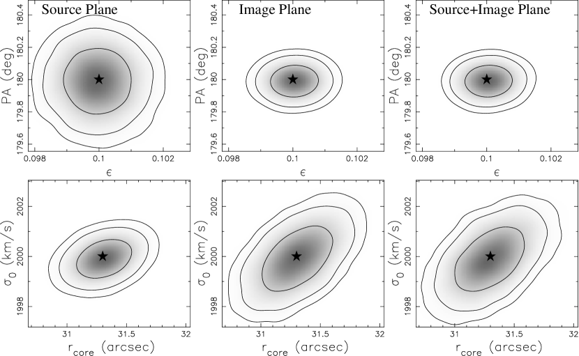
Figure 3 shows that the posterior PDF are similar when computed with the image plane method alone or with the successive source plane+image plane method. However, this latter method is about 8 times faster than the image method alone.

• 

Figure 3: 2D marginalized posterior PDF of a simulated cluster of galaxies. The left, middle and right columns are respectively obtained by computing the likelihood with the source plane method, with the image plane method and successively with the source plane and the image plane methods. In terms of computation time, the combined method source plane – image plane is about 8 times faster than the image plane method alone.

3 A Bayesian Markov Chain Monte Carlo method

We have implemented the Bayesian MCMC package BayeSys (Skilling 2004) to perform the lens model fitting. By model, we mean a multiple-component (and hence multi-scale) mass distribution as described above, with a set of priors for its parameters.

Theoretically, the Bayesian approach is better suited than regression techniques in situations where the data by themselves do not sufficiently constrain the model. In this case, prior knowledge about the parameter Probability Density Function (PDF) helps to reduce the model’s degeneracies. The Bayesian approach is well-suited to strong lens modelling, given the few constraints generally available to optimize a model.

The Bayesian approach provides two levels of inference: parameter space exploration, and model comparison. The first level can be achieved using the unnormalised posterior PDF (equal to the product of the likelihood and the prior); the second requires the calculation of the normalisation of the posterior, known as the evidence. All these quantities are related by Bayes Theorem,

$$\mathrm{Pr}(\boldsymbol{\theta}|D,M)=\frac{\mathrm{Pr}(D|\boldsymbol{\theta},M)\mathrm{Pr}(\boldsymbol{\theta}|M)}{\mathrm{Pr}(D|M)}\;,$$ (11)

where $\mathrm{Pr}(\boldsymbol{\theta}|D,M)$ is the posterior PDF, $\mathrm{Pr}(D|\boldsymbol{\theta},M)$ is the likelihood of getting the observed data $D$ given the parameters $\boldsymbol{\theta}$ of the model $M$, $\mathrm{Pr}(\boldsymbol{\theta}|M)$ is the prior PDF for the parameters, and $\mathrm{Pr}(D|M)$ is the evidence.

The posterior PDF will be the highest for the set of parameters $\boldsymbol{\theta}$ which gives the best fit and is consistent with the prior PDF, regardless of the complexity of the model $M$. Meanwhile, the evidence $\mathrm{Pr}(D|M)$ is the probability of getting the data $D$ given the assumed model $M$. It measures the complexity of model $M$, and, when used as in model selection, it acts as Occam’s razor: “All things being equal, the simplest solution tends to be the best one.” Here, the simplest solution tends to be the model with the smallest number of parameters and with the prior PDF the closest to the posterior PDF. In contrast, the commonly-used reduced $\chi^{2}$ analysis is only a rough approximation to the evidence analysis, although it does provide an absolute estimator of goodness-of-fit (provided the error estimates on the data are accurate).

In information theory, the evidence combines the likelihood and the information $I$, or negative entropy:

$$I=\int\mathrm{Pr}(\boldsymbol{\theta}|D,M)\log(\mathrm{Pr}(\boldsymbol{\theta}|D,M)/\mathrm{Pr}(\boldsymbol{\theta}|M))\mathrm{d}\boldsymbol{\theta}\;.$$ (12)

where the sum is performed over the whole parameter space and $\mathrm{Pr}(\boldsymbol{\theta}|D,M)$ is the posterior PDF and $\mathrm{Pr}(\boldsymbol{\theta}|M)$ is the prior PDF.

The negative entropy measures the information we have obtained in computing the posterior PDF from the input prior PDF. It represents a “distance” between the prior PDF and the posterior PDF. It can also be understood as the volume of the prior PDF over the posterior PDF, which can be very large for high signal to noise data. [In this case the task of parameter space exploration is like searching for a “a needle in a haystack,” and the entropy measures the ratio of the needle’s volume (the posterior PDF) to the haystack’s volume (the prior PDF)].

In general, the information is much bigger than unity because the “distance” between the prior PDF and the posterior PDF is large. For this reason, we use annealed Markov Chains to converge progressively from the prior PDF to the posterior PDF.

Technically, we run 10 interlinked Markov chains at the same time to prevent any Markov chain from falling in a local minimum. The MCMC convergence to the posterior PDF is performed with a variant of the “thermodynamic integration” technique (O Ruanaidh and Fitzgerald 1996) called selective annealing.

“Selective” stands for the following process. At each step, 10 new samples (one per Markov chain) are drawn randomly from the current posterior PDF (which corresponds to the prior PDF at the beginning). These samples are weighted according to their likelihood raised to the power of $\delta_{\lambda}$ (see below) and selected with a variant of the Metropolis-Hasting algorithm (Metropolis et al. 1953; Hastings 1970). Roughly, the samples with the worst likelihood are deleted and the ones with the best likelihood are duplicated so that we always keep $10$ Markov chains running at the same time. Then, bayesys provides 8 exploration algorithms to randomly move the new samples in the parameter space and keep the 10 Markov chains uncorrelated (see Skilling 2004, for more details). This new set of randomly mixed samples is appended to the Markov chains and used as a new seed for the next step.

The bayesys production of new samples is fast but the likelihood computation by lenstool is slow. For each observed image, we must compute the gradient of every potential and sum them to compute the deviation angle and determine the source position. Therefore, the optimization process takes longer with more images and/or more potentials. However, if the $r_{cut}^{\star}$ or $\sigma_{0}^{\star}$ parameters are fixed, the luminosity-scaled subhalo gradients can be computed just once (at the first iteration), thus reducing drastically the computation time.

The “annealing” term of the “selective annealing” technique controls the convergence speed. The slower and smoother the convergence, the more accurate is the evidence and the better-characterised is the posterior. The annealing process is best seen by re-writing Bayes theorem:

$$\mathrm{Pr}(\boldsymbol{\theta}|D,M)=\frac{\mathrm{Pr}(D|\boldsymbol{\theta},M)^{\lambda}\mathrm{Pr}(\boldsymbol{\theta}|M)}{\mathrm{Pr}(D|M)}\;.$$ (13)

Here, $\lambda$ is the cooling factor for the annealing. During a so-called “burn-in” phase, the likelihood influence is raised progressively from $\lambda=0$ to $\lambda=1$ by step of $\delta_{\lambda}\sim\mathrm{Rate}/(\log\mathcal{L}_{max}-\log\bar{\mathcal{L}})$ where $\bar{\mathcal{L}}$ is the mean likelihood value of the 10 samples and Rate is an arbitrary constant set by the user. At the beginning of the optimization, $\delta_{\lambda}$ is small because the likelihood dispersion of the 10 samples is large.

As seen above, the samples are weighted and selected according to their likelihood raised to the power of $\delta_{\lambda}$. Thus, whatever the likelihoods are widely separated, $\delta_{\lambda}$ decreases and the convergence automatically slows in proportion to compensate.

In the small-convergence speed limit, the relative information between the beginning and end of a MCMC step is approximately constant and equals to Rate² (Skilling 2004).

By decreasing Rate, the user decreases the information rate per MCMC step and thus the evidence error (see left panel of Figure 4) but at the price of slower convergence.

Figure 4: Evidence and $\chi^{2}$ evolution in function of the convergence speed parameter “Rate.”

The right panel of Figure 4 shows that, within the error bars, the median $\chi^{2}$ is stable when Rate decreases. A lower Rate implies a slower convergence speed. The chains will contain more samples and hence better explore the parameter space towards the best fit region. This explains the slight decrease of the median $\chi^{2}$ when Rate decreases. Alternatively, the spread of $\chi^{2}$ is similar for all Rate values, indicating that the convergence speed does not affect the parameter space exploration around the median $\chi^{2}$.

From our experience, we have found that a value between 0.1 and 0.5 gives evidence values that are accurate enough for our purposes, while returning the posterior PDF in a reasonable amount of computation time. From Figure 4, we can see that the uncertainty on the logarithm of the evidence is approximately 4 units: this corresponds to an odds ratio of 50 to 1, a sufficiently convincing value. In the rest of this paper, we will use a Rate of 0.1 unless otherwise specified.

3.0.1 MCMC output

Contrary to maximum likelihood methods (like the downhill method used by Kneib et al. 1993), the Bayesian MCMC sampler does not look for the best sample of parameters. Instead, it samples the posterior PDF, drawing more samples where the posterior PDF is higher.

The more samples we collect after the burn-in phase, the better the resolution of the posterior PDF. This is of particular interest given that we use one- and two-dimensional histograms to represent the marginalized posterior PDFs $\mathrm{Pr}(\theta_{i}|M)$ and $\mathrm{Pr}(\theta_{i},\theta_{j}|M)$. The number of histogram bins is limited by the number of samples. To determine the bin sizes, we use the Freedman & Diaconis rule (Freedman and Diaconis 1981). They have shown that in order to get the best fit between a PDF and the corresponding histogram, the bin size should be:

$$\mathrm{Bin\ size}=2\mathrm{IQR}(\theta_{i})N^{-1/3}\;,$$ (14)

where IQR is the interquartile range of the $\theta_{i}$ samples and $N$ is the number of samples.

The produced 2D posterior histograms in the rest of this paper show that the parameters are not independent, and that their PDFs are certainly not Gaussian. Techniques based on the assumption of Gaussian errors, with correlation matrix measured around the best fit, are not accurate and likely underestimate some errors. Therefore, uncertainties must be estimated with care, and eventually asymmetric errors must be adopted in case of large asymmetries observed in the posterior PDF.

To compress the posterior PDFs and provide a convenient way of comparing them, we use the median and the standard deviation estimators. It has been shown (Simard 1996) that the median is the most robust estimator for unimodal asymmetric distributions — which is usually the kind of distribution we have for our parameters — whereas the mean estimator is valid only if the distribution is close to Gaussian. The more samples we have, the less we are affected by outliers.

4 Lens potential parameter degeneracies

In this section, we present and interpret the degeneracies observed in galaxy cluster strong lensing models. Degeneracies will always appear in strong lensing modelling because the lensing only constrains the mass inside an Einstein radius. Unfortunately in parametric models, the parameters involved in the computation of the mass inside the Einstein radius are rarely orthogonal and strongly degenerate.

In the literature, we have found several papers presenting parameters degeneracies (see e.g. Zekser et al. 2006; Rzepecki et al. 2007; Meneghetti et al. 2007, for illustrations of the NFW $r_{s}$—$\rho_{s}$ degeneracy). We are finding similar results, although we are going beyond most of the previous study by exploring many more parameters.

In this section, we use the same potential to simulate and recover the cluster-scale halo, respectively a PIEMD, a NFW and a Sérsic potential. Fitting the data by the true model never happens in practice. However, the presented degeneracies always appear and simple models are required for a proper understanding.

In section 5, we will use different models for the simulation and the recovery in order to compare the limits of each model given the data.

4.1 Description of the simulation

4.1.1 The mass models

We simulate a cluster of galaxies comprising a cluster-scale halo, and 78 galaxy-scale subhalos that perturb the lensing signal. The cluster-scale halo is modelled successively by a PIEMD, a NFW and a Sérsic potential whose input parameters are reported in Table 2. The galaxy-scale subhalos are modelled by PIEMD potentials with vanishing core radius. The cluster is placed at redshift $z=0.2$. Hereafter, we will refer to each model as the PIEMD, the NFW and the Sérsic models.

The galaxy-scale subhalo distribution follows the galaxy distribution in the cluster Abell 2390 in a region of 200 kpc around the cluster centre. This is two times larger than the radius of the outermost images in our simulation. Thus, we account for the shearing effect produced by outer galaxies. The selected galaxies are part of the cluster red-sequence and therefore are assumed to be cluster members.

The galaxy-scale subhalos $r_{cut}$ and $\sigma_{0}$ are scaled with the scaling relations (4). A constant M/L ratio is assumed. We consider the scaling parameters $r_{cut}^{\star}=18$ kpc and $\sigma_{0}^{\star}=200$ km/s as the input values for our simulations. These values correspond to measured values obtained through galaxy-galaxy lensing in Abell 2390 (Natarajan et al. 2006). The apparent K-band magnitude of an $L^{*}$ galaxy at the cluster redshift is $M^{\star}=17.05$ (in AB magnitude) (de Propris et al. 1999). The galaxy magnitudes come from observations of Abell 2390 in the K-band (Jullo et al. 2007), and are used to calculate the true mass parameters in the simulations.

We also include a cD galaxy in the model to produce more systems of multiple images in the cluster centre. The cD galaxy is described by an individual subhalo modelled by a PIEMD potential with vanishing core, and shape parameters matching the light distribution. Its mass profile is characterized by $\sigma_{0}=290.$ km/s, $r_{core}=0$ and $r_{cut}=38.$ kpc. The cluster Einstein radius for a $z=10$ background source is 30.” The enclosed mass at this radius is $M_{eins}=6.7\ 10^{13}\ M_{\odot}$, of which the galaxies’ contribution is about 9%.

• PIEMD	$\epsilon_{\Sigma}$	=	0.3	$r_{core}$ =	40. kpc
  	$PA$	=	127.	$r_{cut}$ =	900. kpc
  				$\sigma_{0}$ =	950. km/s
  NFW	$\epsilon_{\varphi}$	=	0.2	$r_{200}$ =	1800. kpc
  	$PA$	=	127.	$c$ =	6
  Sérsic	$\epsilon_{\varphi}$	=	0.2	$R_{e}$ =	1500. kpc
  	$PA$	=	127.	$\Sigma_{e}$ =	$5\ 10^{7}$ M⊙/kpc2
  				$n$ =	2.8
  $L^{\star}$ galaxy	$r_{cut}^{\star}$	=	18. kpc	$\sigma_{0}^{\star}$ =	200. km/s

Table 2: Input parameters for the 3 simulated cluster-scale components.

4.1.2 Strong lensing constraints

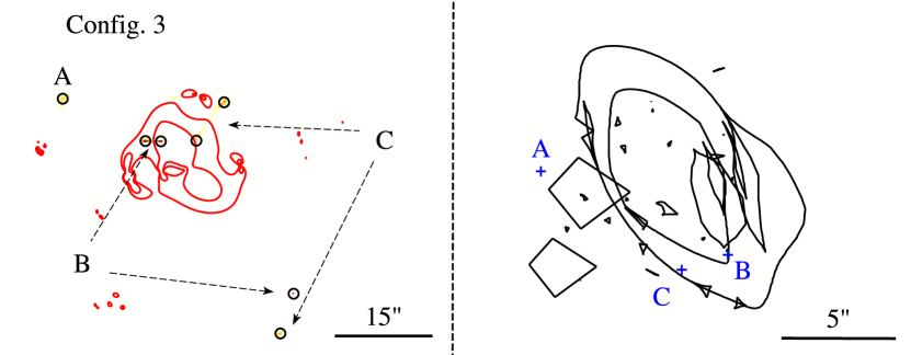
We lens three background sources, $A$, $B$ and $C$, at redshifts $z_{A}=0.6$, $z_{B}=1.0$ and $z_{C}=4.0$, through each simulated cluster. We adjust the $B$ and $C$ source positions in order to produce the three following configurations of multiple images.

Figure 5: Left panel: Image plane for the PIEMD simulated cluster, showing the image positions of the systems $A$, $B$ and $C$ at redshifts $z_{A}=0.6$, $z_{B}=1.0$ and $z_{C}=4.0$ in the configurations 1, 2 and 3. The black circles mark the image positions. The critical curves of systems $B$ and $C$ are shown in red. Right panel: The corresponding source plane. The blue crosses mark the source positions; the caustic curves are plotted in black. The plotted caustics for systems $B$ and $C$ are radial and tangential, tangential and tangential and radial and radial respectively for configurations 1, 2 and 3. North is up and East is left in both panels.

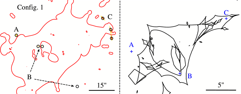
Configuration 1: source $A$ is placed on the North-East side of the cluster, but outside of the multiple image region. It therefore produces a single image. Also on the East side, but inside the radial caustic, source $B$ produces a radial arc system with 3 images. On the West side, source $C$ lies along the West naked cusp of the caustics and so produces a system with 3 tangential images.

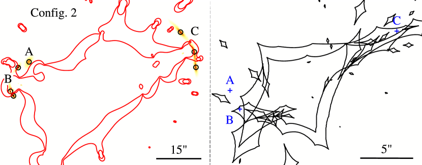
Configuration 2: sources $A$ and $C$ are in the same places as in Config. 1, but source $B$ is placed along the East naked cusp and so produces 3 tangential images. The second configuration therefore constrain mainly the enclosed mass in the outer part of the cluster ($100<r<200$ kpc).

Configuration 3: sources $A$ and $B$ are at the same place as in Config. 1, but source $C$ is placed close to the radial caustics and therefore produces a second radial system of 3 images on the West side of the cluster. The third configuration then preferentially constrains the inner part of the mass profile ($r<100$ kpc).

The source and image positions in the three configurations are presented in Figure 5, along with the critical and caustic curves for sources at redshift $z_{B}=1.0$ and $z_{C}=4.0$. Gaussian noise of FWHM 0.1” was added to the image positions to mimic the observational uncertainties. All the predicted images are used for the parameter recovery unless their lensing magnification is lower than 1. In practice, such images are never observed (too faint or blended in the cD flux).

Config. 1 constrains the cluster central and outer regions, Config. 2 only constrains the outer region and in Config. 3, the 4 radial images strongly constrain the cluster central region on both the East and the West sides.

4.2 PIEMD posterior PDF analysis

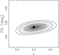
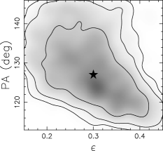
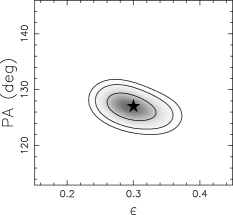
First, we fit the PIEMD model with a PIEMD potential for the cluster-scale halo. For each of the three configurations of multiple images, we recover the cluster-scale halo parameters ($\epsilon$, PA, $r_{core}$, $r_{cut}$ and $\sigma_{0}$), as well as the galaxy-scale subhalos scaling parameters $\sigma_{0}^{\star}$ and $r_{cut}^{\star}$. For each parameter, we assume a uniform prior with 50% errors around its input value. In this case the computed posterior PDF is merely proportional to the likelihood PDF. The cD galaxy subhalo parameters are fixed to their input value in order to avoid annoying additional degeneracies with the cluster-scale halo parameters. We therefore constrain 7 free parameters with 8 constraints. The $\chi^{2}$ is computed in the image plane, although we observed no difference between the source plane $\chi^{2}$ and the image plane $\chi^{2}$.

Figure 6: 2D marginalized posterior PDFs for the parameters of the cluster-scale halo modelled with a PIEMD potential obtained, from left to right, with multiple image configurations 1, 2 and 3 respectively. The 3 contours stand for the 68%, 95% and 99% CL. The input values to the simulation are marked by the stars. The mass of an $L^{\star}$ galaxy is the total mass for a circular profile. The plotted contours in the $r_{cut}^{\star}$–$\sigma_{0}^{\star}$ plot are isodensity contours. The cluster mass $M_{eins}$ is the inferred total enclosed mass (i.e. galaxy subhalos and cluster-scale halo) within the Einstein radius (30”).

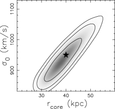
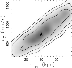
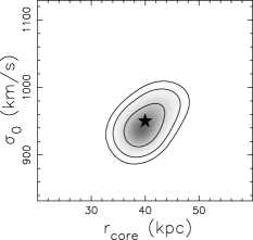
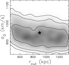
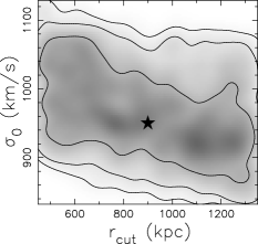
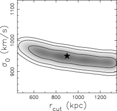
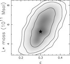
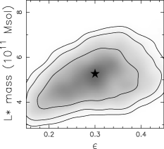
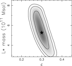
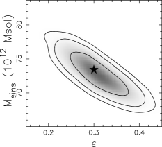
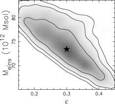
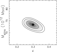
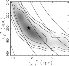
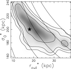
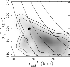
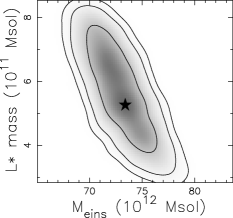
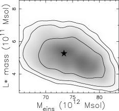
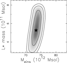
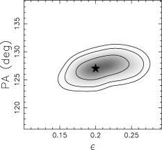
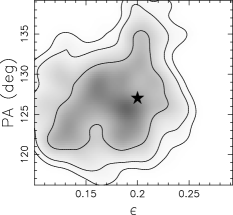
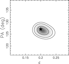
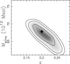
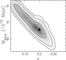
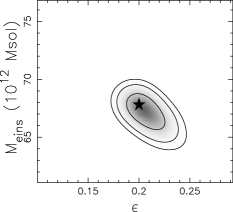
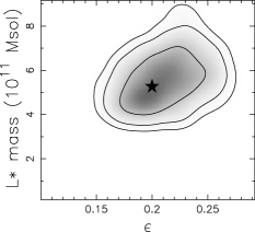
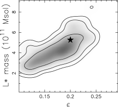
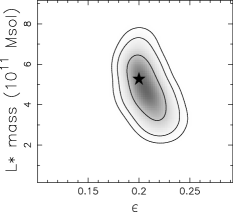
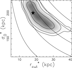
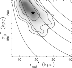
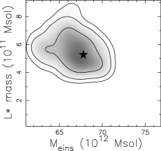
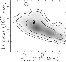
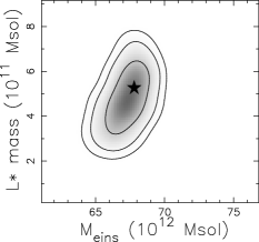
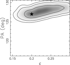
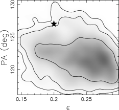
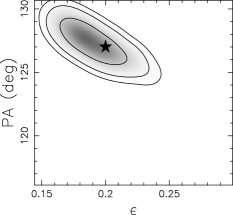
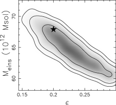
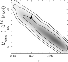
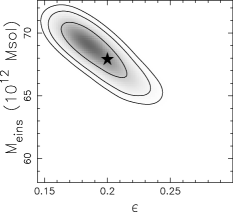
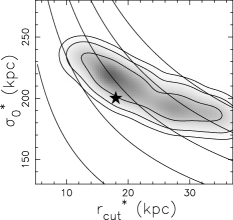
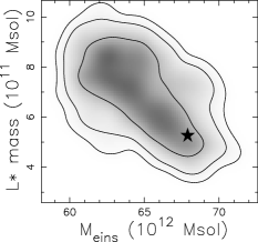
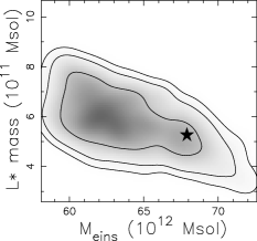
The obtained posterior PDF is marginalized (by making a histogram in two dimensions and ignoring the samples’ other parameters), and plotted in Figure 6. The estimated (median) parameters are given in Table 3. In every configuration, the input values are recovered well, but strong degeneracies appear.

First, we note that the posterior PDF is more compact in Config. 3 than in Config. 1 and 2, in concordance with the number of radial arcs in each configuration. This is in agreement with the results of Miralda-Escude (1995), who showed that the combination of radial arcs and their counter image provides a stringent constraint on the profile shape as well as the enclosed mass.

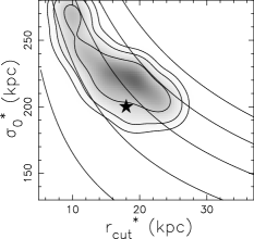
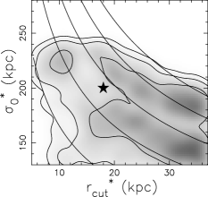
Second, the velocity dispersion tightly correlates with the core radius, and, to a lesser extent, with the cut-off radius. This is a mathematical degeneracy that appears when the mass enclosed by the Einstein radius is maintained constant (or in this case, constrained tightly by the data). Indeed, for a PIEMD potential, the enclosed mass is given by (Limousin et al. 2005):

$$M_{aper}(<R)=\frac{\pi r_{cut}\sigma_{0}^{2}}{G}\left(1-\frac{\sqrt{r_{cut}^{2}+R^{2}}-\sqrt{r_{core}^{2}+R^{2}}}{r_{cut}-r_{core}}\right)\;.$$ (15)

Thus, for a mass enclosed into a large circle of radius $R\sim r_{cut}$, we derive $\sigma_{0}^{2}\propto 1/r_{cut}$. At a smaller radius, assuming $r_{core}\ll r_{cut}$, the 3D density approximates $\rho=\rho_{0}/(1+R^{2}/r_{core}^{2})$ and the corresponding enclosed mass becomes

$$M_{aper}(<R)=\frac{\pi\sigma_{0}^{2}}{G}\left(\sqrt{r_{core}^{2}+R^{2}}-r_{core}\right)\;,$$ (16)

For a constant aperture mass, we then obtain $\sigma_{0}^{2}\propto(\sqrt{r_{core}^{2}+R^{2}}-r_{core})^{-1}$, which is also equivalent to $\sigma_{0}^{2}\propto\frac{1}{R^{2}}(r_{core}+\sqrt{r_{core}^{2}+R^{2}})$, an increasing function of $r_{core}$ resembling the observed degeneracy.

Third, in Config. 3, the cluster-scale cut-off radius is slightly better constrained than in Config. 1 or 2. Since strong lensing cannot probe directly the surface density at the cut-off radius, this result is just a product of the aperture mass definition 15 and the stringent constraints obtained for $r_{core}$ and $\sigma_{0}$.

Fourth, we observe changes in the slopes of the ellipticity–PA, the ellipticity–$L^{\star}$ mass and the $M_{eins}$–$L^{\star}$ mass degeneracies between Config. 1., 2 and 3.

This more effect is due to a subtle interaction between the cluster-scale halo and the galaxy-scale subhalos’ mass distributions during the inference. In particular, in Config. 2, we suggest that when the ellipticity increases, alignment of the cluster with the giant arcs $B$ and $C$ is favoured. However, in Config. 1 and 3, this behaviour is not so clear, probably because of the presence of radial arcs in the central region.

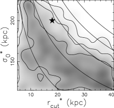
Finally, in every configuration, the scaling relation parameters $r_{cut}^{\star}$ and $\sigma_{0}^{\star}$ are strongly degenerate, with the degeneracy closely following the constant mass contours over-plotted with solid lines. In Table 3, we note that strong lensing cannot predict the $L^{\star}$ cut-off radius to better than 24% accuracy, nor $\sigma_{0}^{\star}$ with better than 6% accuracy.

Although strong degeneracies have been highlighted so far for a cluster-scale halo modelled by a PIEMD potential, the aperture mass error at the Einstein radius is always smaller than 5% and even reaches 0.8% in Config. 3. (see Table 3).

In section 5, we show that the same precision can also be achieved when the input and the fitted models are different.

Table 3: Parameter recovery for a cluster-scale halo modelled by a PIEMD potential, given 3 different strong lensing configurations. The errors are given at 68% CL. The $L^{\star}$ galaxy masses are given for a circular mass component with identical dynamical parameters.

• 	Input	Config.1		Config.2		Config.3
  $\epsilon$	0.3	0.31	$\pm$0.04	0.30	$\pm$0.06	0.29	$\pm$0.02
  $PA$ (deg)	127.	127.2	$\pm$0.9	128.5	$\pm$7.5	127.2	$\pm$0.8
  $r_{core}$ (kpc)	40.	38.8	$\pm$4.7	41.7	$\pm$9.3	39.8	$\pm$1.9
  $\sigma_{0}$ (km/s)	950.	937.3	$\pm$43.9	966.4	$\pm$59.8	946.5	$\pm$16.6
  $r_{cut}$ (kpc)	900.	907.8	$\pm$253.7	894.6	$\pm$264.7	936.5	$\pm$235.7
  $r_{cut}^{\star}$ (kpc)	18.	18.5	$\pm$6.5	19.6	$\pm$6.5	25.9	$\pm$6.3
  $\sigma_{0}^{\star}$ (km/s)	200.	196.9	$\pm$16.8	199.0	$\pm$16.5	180.4	$\pm$12.2
  $M_{L^{\star}}$ ($10^{11}\ M_{\odot}$)	5.26	5.3	$\pm$1.2	5.1	$\pm$0.8	5.7	$\pm$1.1
  $M_{eins}$ ($10^{12}\ M_{\odot}$)	73.4	73.0	$\pm$2.0	74.6	$\pm$3.8	73.5	$\pm$0.6

4.3 NFW posteriors distribution analysis

Now, we fit the NFW model with a NFW potential for the cluster-scale halo. Given the three configurations of multiple images, we perform the recovery of the cluster-scale halo parameters ($\epsilon$, PA, $c$ and $r_{s}$) as well as the galaxy-scale subhalo scaling parameters $\sigma_{0}^{\star}$ and $r_{cut}^{\star}$. Again, we assume uniform priors for the parameters, with a width of 50% centred on the input values; the cD galaxy subhalo parameters are again fixed. We constrain 6 free parameters with 8 constraints.

Figure 7: 2D marginalized posterior PDF of the parameters of the cluster-scale halo modelled with an NFW potential, obtained, from left to right, with multiple-image configuration 1, 2 and 3 respectively. The 3 contours stand for the 68%, 95% and 99% CL . The fiducial values are marked by the stars. The mass of a $L^{\star}$ galaxy is the total mass for a circular profile. The plotted contours in the $r_{cut}^{\star}$–$\sigma_{0}^{\star}$ plot are the isodensity contours. The cluster mass $M_{eins}$ is the total enclosed mass (i.e. galaxy subhalos and cluster-scale halo) in the Einstein radius (30”).

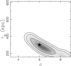
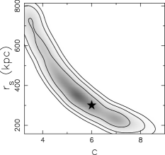
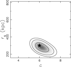
The obtained posterior PDF is marginalized and plotted in Figure 7. The (median) estimated parameters are given in Table 4 as well.

First, similarly to the PIEMD case, we note that the degeneracies are more compact in Config. 3 than in Config. 1 and 2 for which the central region of the cluster is less constrained.

Second, we note a strong degeneracy between $c$ and the $r_{s}$. It can be fitted by a power law $r_{s}\propto c^{\alpha}$ where $\alpha=-1.7$, $-1.5$ and $-1.4$ for Config. 1, 2 and 3 respectively. To confirm the mathematical origin of this degeneracy, we consider the NFW definition of the aperture mass. By solving numerically for $r_{s}$ given $c$ at constant aperture mass, we manage to reproduce the observed degeneracy and measure $\alpha=-1.1$, in relatively good agreement with the measured slopes given the uncertainty on the aperture mass.

Third, the ellipticity, the PA, the $M_{eins}$ and the $L^{\star}$ mass parameters are degenerate in the same manner as in the previous section, when the cluster-scale halo was modelled by a PIEMD potential. This confirms that these degeneracies are independent of the cluster model, and just depend on the lensed image configuration.

Finally, in Table 4, we note that the $L^{\star}$ cut-off radius error is recovered with nearly the same accuracy when the cluster-scale halo is modelled by a NFW potential than when modelled by a PIEMD potential. This suggest that the scaling relation parameters accuracy is model-independent. Similarly, the uncertainty on the enclosed mass measured at the Einstein radius is similar to that found when the cluster-scale halo is modelled by a PIEMD potential.

Table 4: Parameter recovery results for a cluster-scale halo modelled by a NFW potential, given 3 different strong lensing configurations. The errors are given at 68% CL. The $L^{\star}$ masses are given for a circular mass component with identical dynamical parameters.

• 	Input	Config.1		Config.2		Config.3
  $\epsilon$	0.2	0.21	$\pm$0.02	0.18	$\pm$0.03	0.21	$\pm$0.01
  $PA$ (deg)	127.	127.4	$\pm$1.0	126.6	$\pm$4.0	126.6	$\pm$0.6
  $c$	6.	6.5	$\pm$0.9	6.4	$\pm$0.8	5.9	$\pm$0.3
  $Scale\ radius$ (kpc)	300.	269.3	$\pm$54.6	367.9	$\pm$149.9	284.7	$\pm$22.5
  $r_{cut}^{\star}$ (kpc)	18.	21.6	$\pm$4.8	16.3	$\pm$3.9	20.6	$\pm$10.1
  $\sigma_{0}^{\star}$ (km/s)	200.	191.5	$\pm$15.4	205.6	$\pm$13.4	169.6	$\pm$27.8
  $M_{L^{\star}}$ ($10^{11}\ M_{\odot}$)	5.26	5.56	$\pm$1.7	4.2	$\pm$1.1	4.9	$\pm$0.9
  $M_{eins}$ ($10^{12}\ M_{\odot}$)	67.8	66.9	$\pm$1.8	69.5	$\pm$2.9	67.4	$\pm$0.8

4.4 Sérsic posterior distribution analysis

Finally, we fit the Sérsic model with a Sérsic potential for the cluster-scale halo. We perform the recovery of the cluster-scale halo parameters ($\epsilon$, PA, $R_{e}$, $\Sigma_{e}$ and $n$), as well as the galaxy-scale subhalo scaling parameters $\sigma_{0}^{\star}$ and $r_{cut}^{\star}$, given the same three configurations of multiple images as before.

Again, we assume uniform priors for the parameters, with widths of 50% centred on the input values. The cD galaxy subhalo parameters are fixed. We constrain 7 free parameters with 8 constraints.

Figure 8: 2D marginalized posterior PDF of the parameters of the cluster-scale halo modelled with an Sérsic potential obtained from left to right with Config. 1, 2 and 3 of multiple images respectively. The 3 contours stand for the 68%, 95% and 99% CL. The fiducial values are marked by the stars. The mass of a $L^{\star}$ galaxy is the total mass for a circular profile. The plotted contours in the $r_{cut}^{\star}$–$\sigma_{0}^{\star}$ plot are the iso-mass contours. The cluster mass $M_{eins}$ is the total enclosed mass (i.e. galaxy subhalos and cluster-scale halo) in the Einstein radius (30”).

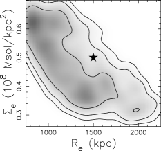
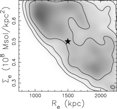
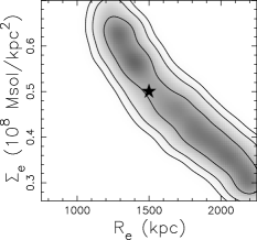
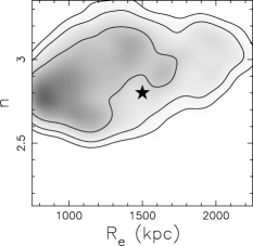
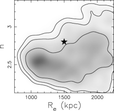
The obtained posterior PDF is marginalized and plotted in Figure 8. The estimated parameters are given in Table 5.

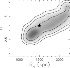
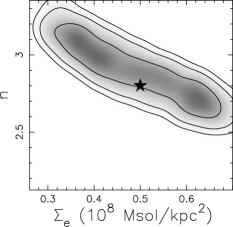
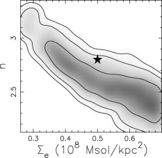
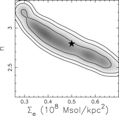
First, we note that for the same lensing configuration, the parameters of a cluster-scale halo modelled by a Sérsic potential are more difficult to constrain than those of a PIEMD or a NFW potential. We understand this to be a result of the effective radius $R_{e}$ and index parameter $n$ mainly impacting the outer region of the mass distribution, which is not probed by strong lensing.

Second, the ellipticity, the PA, the $M_{eins}$ and the $L^{\star}$ mass parameters are degenerate in the same manner as in the previous sections, confirming that these degeneracies are dependent on the lensing configuration alone.

Finally, in Table 5, we note that the $L^{\star}$ cut-off radius is recovered with nearly the same accuracy as in the case where the cluster-scale halo is modelled with the NFW potential. We suggest therefore that the scaling parameters $r_{cut}^{\star}$ and $\sigma_{0}^{\star}$ accuracies cannot be lower than about 20% and 7% respectively. This result is independent of both the model and the lensing configuration.

Table 5: Parameter recovery results for a cluster-scale halo modelled by a Sérsic potential and recovered in 3 different strong lensing configurations. The errors are given at 68% CL. The $L^{\star}$ masses are given for a circular mass component with identical dynamical parameters.

• 	Input	Config.1		Config.2		Config.3
  $\epsilon$	0.2	0.23	$\pm$0.03	0.24	$\pm$0.04	0.19	$\pm$0.01
  $PA$ (deg)	127.	128.0	$\pm$0.8	121.9	$\pm$2.3	127.5	$\pm$1.0
  $R_{e}$ (kpc)	1500.	1195.7	$\pm$345.5	1630.8	$\pm$372.4	1698.5	$\pm$319.3
  $\Sigma_{e}$ ($10^{8}\ M_{\odot}$)	0.5	0.5	$\pm$0.1	0.5	$\pm$0.1	0.5	$\pm$0.1
  $n$	2.8	2.9	$\pm$0.2	2.6	$\pm$0.2	2.8	$\pm$0.2
  $r_{cut}^{\star}$ (kpc)	18.	21.0	$\pm$3.3	16.8	$\pm$4.2	25.4	$\pm$8.2
  $\sigma_{0}^{\star}$ (km/s)	200.	206.6	$\pm$15.5	223.6	$\pm$20.2	178.0	$\pm$29.2
  $M_{L^{\star}}$ ($10^{11}\ M_{\odot}$)	5.26	6.9	$\pm$1.3	5.9	$\pm$0.9	6.1	$\pm$1.2
  $M_{eins}$ ($10^{12}\ M_{\odot}$)	67.9	64.6	$\pm$2.0	65.5	$\pm$3.4	68.8	$\pm$1.3

Figure 9 sums up the results found in this section concerning the accuracy obtained on the mass profile in each configuration for each potential. Although the accuracy depends on the lensing configuration it is usually better than 5% in the region of multiple images with no obvious bias. The accuracy is model independent, and is just the noise on the image positions (0.1 arcsec) translated into the uncertainty on the parameters.

• 

Figure 9: Relative mass profile recovery in the three configurations for the three potentials PIEMD(vertically hatched region), NFW($-45^{\circ}$ hatched region) and Sérsic($45^{\circ}$ hatched region). The arrows below each plot mark the positions of the multiple images used as constraints. The error bars are given at 68% CL.

5 Model inference

In this section, we use the Bayesian evidence to rank models. As an example, we consider the controversial inner slope of the density profile in clusters of galaxies. In 2004, Sand et al. have used a sample of 6 galaxy clusters to show that the slope of the central density profile was shallower than $r^{-1}$ as predicted by CDM simulations. In their modelling they were using axisymmetric potentials. The same year, Bartelmann and Meneghetti reconsider these results and conclude that an NFW profile with a $r^{-1}$ inner slope could not be ruled out by strong lensing once effects of asymmetry and shear were taken into account.

In order to illustrate the model inference with the Bayesian evidence, we assume here that galaxy clusters actually present an inner slope shallower than $r^{-1}$. Then, we show that even when accounting for asymmetry and shear, the Bayesian evidence is still able to rank models and eventually rule them out.

To do so, as an input model, we use the PIEMD model from section 4.2 i.e. the inner slope is shallower than $r^{-1}$. In order to observe the limits of Bayesian inference with the evidence, we simulate 6 models in which we change the size of the cluster-scale halo core radius. We scale the velocity dispersion accordingly so that the enclosed mass at the Einstein radius is maintained.

The 3 background galaxies of the previous section are lensed through each model. We have to slightly move the sources in the source plane so that in every simulation, we always end up with 1 tangential system, 1 radial system and 1 singly imaged system. For models with $r_{core}<30$ kpc, we remove the images predicted at the very centre of the galaxy cluster because their lensing amplification is lower than 1 and in practice they are never observed (either too faint or blended in the cD galaxy flux). In contrast, for models with $r_{core}\geq 30$ kpc, we keep all the predicted images because their lensing amplification is always greater than 1. We add a Gaussian noise of FWHM 0.1” to each image position.

Then, we successively fit a SIE, a NFW and a Sérsic potential to the simulated systems of multiple images and report the computed evidences in Table 6. As a reference, the last column reports the evidence computed when we fit the simulated PIEMD models by themselves. We assume no prior knowledge (in practice, we use uniform distributions and adjust the limits so that the posterior PDF is not bounded). We also consider the scaling relation parameters $r_{cut}^{\star}$ and $\sigma_{0}^{\star}$ as free parameters.

• 

Figure 10: Aperture mass profile errors relative to the input PIEMD mass profile for the fitted potentials SIE (vertically hatched region), NFW ($-45^{\circ}$ hatched region) and Sérsic ($45^{\circ}$ hatched region) as a function of the aperture radius. The hatched width represents the 3$\sigma$ error estimated from the posterior PDF. The arrows mark the positions of the multiple images used as constraints.

Figure 10 shows the aperture mass errors relative to the input PIEMD mass profile for the SIE, the NFW and the Sérsic potentials.

First, we note that excluding the inner region and when $r_{core}\leq 20$ kpc, the input mass profile is well recovered by all the models. Note that in the case $r_{core}=0$ kpc, the SIE aperture mass error is smaller than 10% on the full range of radius. This ascertain the consistency of our SIE and PIEMD models. Conversely, the SIE aperture mass error increases rapidly in the inner region as soon as we increase the core radius. In the inner region, the large errors are due to the intrinsic slope of each model (see Figure 1).

The evidences reported in Table 6 correctly summarize these observations. In particular, the SIE evidence at $r_{core}=0$ kpc is close to the evidences of the other models. According to Jeffreys (1961), the difference between two models is substantial if $1<\Delta\ln E<2.5$, strong if $2.5<\Delta\ln E<5$ and decisive if $\Delta\ln E>5$. Following this criteria, for $r_{core}\leq 20$ kpc, the NFW, the Sérsic and the SIE models are equivalent at fitting the data within the evidence error established in section 3. However, when the core radius increases, the SIE model can be confidently rejected.

Now, excluding the SIE models, we can use the evidences to classify the models in 2 categories : (i) when $r_{core}\leq 20$ kpc, the NFW and the Sérsic models evidences are equivalent to the reference PIEMD evidence within the evidence error. The evidences cannot confidently rank models. (ii) when $r_{core}>20$ kpc, the evidences drop significantly and the NFW and Sérsic models are confidently ruled out. This corresponds to the appearance of bright images inside the core radius (see Figure 10) as expected from flat core models. Here, the Sérsic model evidences are generally better than the NFW model evidences although the Sérsic model contains an additional free parameter. In the $r_{core}=30$ kpc case, the NFW and the Sérsic models evidences are very low because of the stringent constraints imposed by the distribution of multiple images (a triplet of tangential images at $R=81$ kpc and a set of uniformly distributed images below 40 kpc).

Finally, we conclude that the Bayesian evidence can effectively rank strong lensing models even when accounting for asymmetry and shear. However, this result strongly depends of the presence of images in the cluster centre.

As we are submitting this paper, some of us are already using lenstool and the evidence inference to study the inner slope of the dark matter profile with real data. Their results will be published in a forthcoming paper.

Table 6: Comparison of the log(Evidence) produced by the fit of the NFW, SIE and Sérsic potentials to a core radius varying PIEMD potential. The values come from fits performed with sets of multiple images described in the text and a Rate equal to 0.1

• Core radius (kpc)	$E_{NFW}$	$E_{Sersic}$	$E_{SIE}$	$E_{PIEMD}$
  0	-27.	-25.	-28.	-20.
  10	-25.	-23.	-33.	-19.
  20	-27.	-24.	-146.	-19.
  30	-198.	-204.	-1391.	-25.
  40	-81.	-70.	-2795.	-19.
  50	-86.	-73.	-3260.	-22.

6 Conclusion

In this study, we have described how to build a gravitational lensing model of galaxy clusters and a set of constraints with multiply and singly imaged systems. Then, we have presented a new Bayesian method for efficiently exploring its parameter space without falling into local maxima of the likelihood PDF. The Bayesian method also gives an estimate of the errors and includes prior knowledge. We have illustrated the Bayesian posterior PDF analysis by studying the degeneracies in the PIEMD, the NFW and the Sérsic potentials in 3 different configurations of multiple images. We draw the following conclusions.

(i) Strong degeneracies appear in both the PIEMD, the NFW and the Sérsic potentials. The parameters are clearly dependent and compensate in order to produce a constant enclosed mass at the images location. The degeneracies are either due to the mathematical definitions of the potentials ($\sigma_{0}$–$r_{core}$, $\sigma_{0}$–$r_{cut}$ for PIEMD, $c$–$r_{s}$ for NFW, $R_{e}$–$\Sigma_{e}$, $R_{e}$–$n$ and $\Sigma_{e}$–$n$ for Sérsic) or to the configuration of multiple images ($\epsilon$–$PA$, $\epsilon$–$L^{\star}$ galaxy mass, $M_{eins}$–$L^{\star}$ galaxy mass). The latter degeneracies are easily identified by looking at the degeneracies between the shape and the dynamical parameters. They are model independent. In every case, the enclosed mass in the Einstein radius decreases with the model ellipticity.

(ii) Radial systems of multiple images combined to tangential arcs provide unique constraints on the slope of the mass profile. It is therefore important to identify radial (or central) images in the cluster cores.

(iii) The PIEMD cut-off radius, the Sérsic effective radius and the NFW scale radius are poorly constrained by strong lensing only. Hopefully, future parametric methods combining weak and strong lensing will provide tighter constraints.

(iv) Galaxy-scale subhalos degenerate with the cluster-scale halo. The best constraints were obtained in lensing configurations combining radial and tangential multiple images systems. In this case, we barely manage a 20% accuracy on the cut-off radius of subhalos scaled with scaling relations. As shown by (Natarajan et al. 1998, 2006) weak and strong lensing combination can improve this result.

We have also illustrated how to rank models with the Bayesian evidence. We fit a NFW, a Sérsic and a SIE potential to 6 PIEMD simulated clusters with different core radius. We have shown that the NFW and the Sérsic potentials can actually fit systems of multiple images produced by clusters with core radius provided no image lie inside the core radius. For large core radius, central images appear at the very centre of the cluster and provide enough constraints to disentangle PIEMD, NFW or Sérsic based models.

Although strong lensing is a wonderful tool to infer surface densities, it becomes rapidly limited by the models and the observed lensing configuration. For instance, it is not possible to constrain the central density slope without radial images. Actually, the presence of radial images strongly suggests the presence of a flat core.

In a forthcoming paper, we will expand this method to constrain cosmological parameters with strong lensing. With a large number of multiple images with known redshift, one should be able to compare the strong lensing cosmography constraints (similarly to the early work of Golse et al. (2002) and Soucail et al. (2004)) with other methods such as the CMB/WMAP results, or Supernovae or cosmic shear results.

Appendix A Critical lines computation with Marching squares

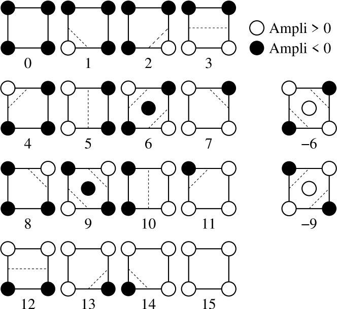
A multiscale marching squares technique has been implemented in lenstool to compute the critical lines. Marching squares is a computer graphics algorithm that generates contour lines for a 2D scalar field. It is similar to the marching cubes algorithm (Lorensen and Cline 1987). The algorithm proceeds through a scalar field taking four neighbour locations at a time (thus forming an imaginary square), then determining the line needed to represent the part of the contour that passes through this square. The individual lines are then fused into the desired contour.

This is done by creating an index to a precalculated array of 16 ($2^{4}=16$) possible line configurations within the square (see Figure 11), by treating each of the 4 scalar values as a bit in an 4-bit integer. If the scalar’s value is higher than the iso-value (i.e. it is inside the contour) then the appropriate bit is set to one, while if it is lower (outside), it is set to zero. The final value after all 4 scalars are checked, is the actual index to the line configuration array.

• 

Figure 11: 16 square configurations. The empty and filled circles are points with positive and negative amplification respectively. The dashed lines are the infered critical lines.

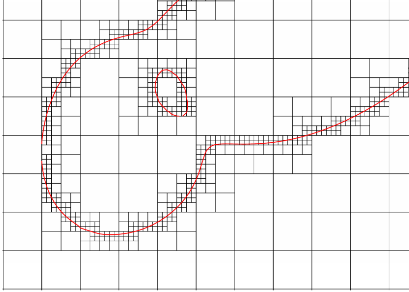
In the critical lines case, the scalar field is not known a-priori. Therefore, we adopt a multiscale algorithm to focus towards the critical lines. The field is split in two recursively until we reach a higher limit for the size of a rectangle. Then, if a critical line is detected in a rectangle, it is split further. The rectangles with no critical line detected are left aside. Once the size of the rectangle has reached a lower limit, a line is kept in memory for this rectangle according to the marching squares configurations. The individual lines are then fused into the critical lines contour.

The previous technique was a line following algorithm called snake. It starts from the center of a clump and picks amplification samples along its way outwards. When an amplification sign change is encountered, it precises the infinite amplification position and circles the clump until it comes back to its starting point along the critical line.

In complex environment, the snake algorithm sometimes gets lost and produces incomplete critical lines. Conversely, the multiscale marching square algorithm never gets lost and identifies all the critical lines in the field. However, it can miss a part of critical line if the higher limit is too large.

• 

Figure 12: Multiscale marching square field splitting. The boxes represent the splitting squares and the red lines, the critical curve contour. The imposed upper and lower limits for the boxes sizes are 10” and 1” respectively. The 1” boxes are not plotted for clarity.

Appendix B Pseudo-elliptical Sérsic potential

As another addition to lenstool, we have incorporated the Sérsic density profile (Sérsic 1968) as an alternative description of the matter density. The motivation for including it is that as the Sérsic profile describes the 2D luminosity profile of elliptical galaxies (Sérsic 1968; Ciotti 1991; Caon et al. 1993), it can be used to separately model the baryonic matter component (which should be traced by the light) and the dark matter (DM) component, given enough lensing constraints. In addition, Merritt et al. (2005, 2006), find that a deprojected Sérsic profile gives a better fit than an NFW profile to the 3D density profile of DM halos from simulations. Elíasdóttir and Möller (2007) found that given that the surface density distribution is indeed given by a Sérsic profile, but fitted by an NFW using lensing constraints, it can lead to unrealistic estimates of the parameters (e.g. the predicted weak lensing signal and the concentration parameter), making the Sérsic profile an interesting alternative for modelling the DM halos themselves. Finally, the special case of the Sérsic index $n=1$, corresponds to an exponential disk, making it useful for modelling spiral galaxies. Spiral lenses are comparatively rare to date, but dedicated efforts are being made to find such lenses, and with the inclusion of the Sérsic profile to Lenstool, it can now be used to study and model such lenses.

The Sérsic 2D density profile has three free parameters ($n,R_{e},\Sigma_{e}$) and is given by:

$$\Sigma_{\mathrm{ser}}=\Sigma_{e}\exp\left[-b_{n}\left(\left(\frac{R}{R_{e}}\right)^{1/n}-1\right)\right]\;,$$ (17)

where $R$ is the projected radius, $n$ is the Sérsic index, $b_{n}$ is a constant chosen such that $R_{e}$ is the radius containing one-half of the projected mass and $\Sigma_{e}$ is the density at $R_{e}$. The Sérsic profile reduces to the de Vaucouleurs profile for $n=4$, and to the exponential disk for $n=1$. The other parameters of the Sérsic profile in lenstool are its position on the sky, its position angle and its ellipticity.

The elliptic version of the Sérsic profile is calculated using the pseudo-elliptical approximation developed by Golse et al. (2002). It is introduced in the expression of the circular Sérsic potential by substituting $R$ by $R_{\epsilon}$, using the following elliptical coordinate system:

$$\left\{\begin{array}[]{l}x_{\epsilon}=\sqrt{(1-\epsilon)}x\\ y_{\epsilon}=\sqrt{(1+\epsilon)}y\\ R_{\epsilon}=\sqrt{x_{\epsilon}^{2}+y_{\epsilon}^{2}}\\ \phi=\arctan(y_{\epsilon}/x_{\epsilon})\;.\end{array}\right.$$ (18)

In this definition, $\epsilon=(a^{2}-b^{2})/(a^{2}+b^{2})$ where $a$ and $b$ are respectively the semi-major and the semi-minor axis of the elliptical potential. From the elliptical lens potential $\varphi_{\epsilon}(r)\equiv\varphi(r_{\epsilon})$, Golse et al. propose generic expressions to compute the elliptical deviation angle $\boldsymbol{\alpha}_{\epsilon}(\mathbf{r})$, the convergence $\kappa_{\epsilon}(\mathbf{r})$, the shear $\gamma_{\epsilon}(\mathbf{r})$ and the projected mass density $\Sigma_{\epsilon}(\mathbf{r})$:

$$\Sigma_{\epsilon}(\mathbf{r})=\Sigma(r_{\epsilon})+\epsilon\cos 2\phi_{\epsilon}(\bar{\Sigma}(r_{\epsilon})-\Sigma(r_{\epsilon}))\;.$$ (19)

The pseudo-elliptical developments are limited to small ellipticities. For instance for the NFW, when $\epsilon>0.25$, the surface iso-densities become increasingly boxy/peanut. Similarly for the Sérsic potential, we have found that when $\epsilon>0.25$, the goodness of fit (defined in Golse et al.) measured at $R_{\epsilon}=R_{e}$ becomes larger than 10%. We also fit the relation between $\epsilon_{\Sigma}$ and $\epsilon$ and found $\epsilon_{\Sigma}=3.55\epsilon-3.42\epsilon^{2}$ with a $\chi^{2}=10^{-5}$.

The ellipticities of the potentials used in this paper and of the projected mass densities $\epsilon_{\Sigma}$ are linearly proportional through multiplicative factors (reported in Table 1).

The range of valid surface density axis ratio $q=b/a$ provided by the pseudo-elliptical approximation for the SIE, the NFW and the Sérsic potentials are $q_{SIE}>0.65$, $q_{NFW}>0.53$ and $q_{Sersic}>0.44$ respectively. From N-body simulations Oguri et al. (2003) found that the most probable projected axis ratio is $q=0.6$. The pseudo-elliptical technique is therefore able to model most of the triaxial halos.

In case of highly elliptical mass distributions, the PIEMD model (Kassiola and Kovner 1993) produces elliptical iso-densities because the ellipticity has been introduced directly in the projected mass distribution and not at the level of the potential.

References

- (1)
- Abdelsalam et al. (1998) Abdelsalam H M, Saha P and Williams L L R 1998 MNRAS 294, 734–+.
- Bardeau et al. (2005) Bardeau S, Kneib J P, Czoske O, Soucail G, Smail I, Ebeling H and Smith G P 2005 A&A 434, 433–448.
- Bartelmann and Meneghetti (2004) Bartelmann M and Meneghetti M 2004 A&A 418, 413–418.
- Blandford and Narayan (1986) Blandford R and Narayan R 1986 ApJ 310, 568–582.
- Bradač et al. (2005) Bradač M, Schneider P, Lombardi M and Erben T 2005 A&A 437, 39–48.
- Brainerd et al. (1996) Brainerd T G, Blandford R D and Smail I 1996 ApJ 466, 623–+.
- Broadhurst et al. (2005) Broadhurst T, Benítez N, Coe D and et al 2005 ApJ 621, 53–88.
- Cabanac et al. (2007) Cabanac R A, Alard C, Dantel-Fort M, Fort B, Gavazzi R, Gomez P, Kneib J P, Le Fèvre O, Mellier Y, Pello R, Soucail G, Sygnet J F and Valls-Gabaud D 2007 A&A 461, 813–821.
- Caon et al. (1993) Caon N, Capaccioli M and D’Onofrio M 1993 MNRAS 265, 1013–+.
- Ciotti (1991) Ciotti L 1991 A&A 249, 99–106.
- Ciotti and Bertin (1999) Ciotti L and Bertin G 1999 A&A 352, 447–451.
- Clowe and Schneider (2001) Clowe D and Schneider P 2001 A&A 379, 384–392.
- Comerford and Natarajan (2007) Comerford J M and Natarajan P 2007 ArXiv Astrophysics e-prints .
- Corless and King (2006) Corless V and King L 2006 ArXiv Astrophysics e-prints .
- de Propris et al. (1999) de Propris R, Stanford S A, Eisenhardt P R, Dickinson M and Elston R 1999 AJ 118, 719–729.
- Diego et al. (2005) Diego J M, Sandvik H B, Protopapas P, Tegmark M, Benítez N and Broadhurst T 2005 MNRAS 362, 1247–1258.
- Dominik (1995) Dominik M 1995 Astronomy and Astrophysics, Supplement 109, 597–+.
- Dye and Warren (2005) Dye S and Warren S J 2005 ApJ 623, 31–41.
- Elíasdóttir and Möller (2007) Elíasdóttir Á and Möller O 2007 Journal of Cosmology and Astro-Particle Physics 7, 6–+.
-
Freedman and Diaconis (1981)
Freedman D and Diaconis P 1981 Probability Theory and
Related Fields 57, 453–476.
http://www.springerlink.com/content/mp364022824748n3 - Gavazzi et al. (2003) Gavazzi R, Fort B, Mellier Y, Pelló R and Dantel-Fort M 2003 A&A 403, 11–27.
- Golse (2002) Golse G 2002 Strong Lensing PhD thesis Université Paul Sabatier, Toulouse III, France.
- Golse and Kneib (2002) Golse G and Kneib J P 2002 A&A 390, 821–827.
- Golse et al. (2002) Golse G, Kneib J P and Soucail G 2002 A&A 387, 788–803.
- Halkola et al. (2006) Halkola A, Seitz S and Pannella M 2006 MNRAS pp. 1133–+.
- Hastings (1970) Hastings W 1970 Biometrika 57, 97–109.
- Ilbert et al. (2006) Ilbert O, Arnouts S, McCracken H J, Bolzonella M, Bertin E, Le Fèvre O, Mellier Y, Zamorani G, Pellò R, Iovino A, Tresse L, Le Brun V, Bottini D, Garilli B, Maccagni D, Picat J P, Scaramella R, Scodeggio M, Vettolani G, Zanichelli A, Adami C, Bardelli S, Cappi A, Charlot S, Ciliegi P, Contini T, Cucciati O, Foucaud S, Franzetti P, Gavignaud I, Guzzo L, Marano B, Marinoni C, Mazure A, Meneux B, Merighi R, Paltani S, Pollo A, Pozzetti L, Radovich M, Zucca E, Bondi M, Bongiorno A, Busarello G, de La Torre S, Gregorini L, Lamareille F, Mathez G, Merluzzi P, Ripepi V, Rizzo D and Vergani D 2006 A&A 457, 841–856.
- Jeffreys (1961) Jeffreys H 1961 Theory of Probability 3 edn Oxford University Press.
- Jørgensen et al. (1996) Jørgensen I, Franx M and Kjaergaard P 1996 MNRAS 280, 167–185.
- Jullo et al. (2007) Jullo E et al. 2007 in prep. .
- Kassiola and Kovner (1993) Kassiola A and Kovner I 1993 ApJ 417, 450–+.
- King and Corless (2007) King L and Corless V 2007 MNRAS 374, L37–L41.
- King et al. (2002) King L J, Clowe D I and Schneider P 2002 A&A 383, 118–124.
- Kneib et al. (2003) Kneib J, Hudelot P, Ellis R S, Treu T, Smith G P, Marshall P, Czoske O, Smail I and Natarajan P 2003 ApJ 598, 804–817.
- Kneib et al. (1996) Kneib J P, Ellis R S, Smail I, Couch W J and Sharples R M 1996 ApJ 471, 643–+.
- Kneib et al. (1993) Kneib J P, Mellier Y, Fort B and Mathez G 1993 A&A 273, 367–+.
- Kochanek (2006) Kochanek C S 2006 in G Meylan, P Jetzer, P North, P Schneider, C. S Kochanek and J Wambsganss, eds, ‘Saas-Fee Advanced Course 33: Gravitational Lensing: Strong, Weak and Micro’ pp. 91–268.
- Koopmans (2005) Koopmans L V E 2005 MNRAS 363, 1136–1144.
- Koopmans et al. (2006) Koopmans L V E, Treu T, Bolton A S, Burles S and Moustakas L A 2006 ApJ 649, 599–615.
- Limousin et al. (2005) Limousin M, Kneib J P and Natarajan P 2005 MNRAS 356, 309–322.
- Limousin et al. (2006) Limousin M, Kneib J P and Natarajan P 2006 ArXiv Astrophysics e-prints .
- Limousin et al. (2007) Limousin M, Richard J, Jullo E, Kneib J P, Fort B, Soucail G, Elíasdóttir A, Natarajan P, Ellis R S, Smail I, Czoske O, Smith G P, Hudelot P, Bardeau S, Ebeling H, Egami E and Knudsen K K 2007 ApJ 668, 643–666.
- Lorensen and Cline (1987) Lorensen W E and Cline H E 1987 in ‘SIGGRAPH’ pp. 163–169.
- Lynds and Petrosian (1986) Lynds R and Petrosian V 1986 in ‘Bulletin of the American Astronomical Society’ pp. 1014–+.
- Marshall et al. (2002) Marshall P J, Hobson M P, Gull S F and Bridle S L 2002 MNRAS 335, 1037–1048.
- Meneghetti et al. (2007) Meneghetti M, Bartelmann M, Jenkins A and Frenk C 2007 MNRAS pp. 781–+.
- Merritt et al. (2006) Merritt D, Graham A W, Moore B, Diemand J and Terzić B 2006 AJ 132, 2685–2700.
- Merritt et al. (2005) Merritt D, Navarro J F, Ludlow A and Jenkins A 2005 ApJ 624, L85–L88.
- Metropolis et al. (1953) Metropolis N, Rosenbluth A, Rosenbluth M, Teller A and Teller E 1953 J. Chemical Physics 21(6), 1087–1092.
- Miralda-Escude (1995) Miralda-Escude J 1995 ApJ 438, 514–526.
- Muñoz et al. (1998) Muñoz J A, Falco E E, Kochanek C S, Lehár J, McLeod B A, Impey C D, Rix H W and Peng C Y 1998 Astrophysics and Space Science 263, 51–54.
- Natarajan et al. (2006) Natarajan P, De Lucia G and Springel V 2006 ArXiv Astrophysics e-prints .
- Natarajan and Kneib (1997) Natarajan P and Kneib J P 1997 MNRAS 287, 833–847.
- Natarajan et al. (1998) Natarajan P, Kneib J P, Smail I and Ellis R S 1998 ApJ 499, 600–+.
- Natarajan et al. (2002) Natarajan P, Loeb A, Kneib J P and Smail I 2002 ApJ 580, L17–L20.
- Navarro et al. (1997) Navarro J F, Frenk C S and White S D M 1997 ApJ 490, 493–+.
- O Ruanaidh and Fitzgerald (1996) O Ruanaidh J J K and Fitzgerald W J 1996 Numerical Bayesian methods applied to signal processing Statistics and Computing Series Springer New York.
- Oguri et al. (2003) Oguri M, Lee J and Suto Y 2003 ApJ 599, 7–23.
- Paczynski (1987) Paczynski B 1987 Nature 325, 572–+.
- Press et al. (1986) Press W H, Flannery B P and Teukolsky S A 1986 Numerical recipes. The art of scientific computing Cambridge: University Press, 1986.
- Richard et al. (2007) Richard J, Kneib J P, Jullo E, Covone G, Limousin M, Ellis R, Stark D, Bundy K, Czoske O, Ebeling H and Soucail G 2007 ArXiv Astrophysics e-prints .
- Rzepecki et al. (2007) Rzepecki J, Lombardi M, Rosati P, Bignamini A and Tozzi P 2007 A&A 471, 743–752.
- Saha and Williams (1997) Saha P and Williams L L R 1997 MNRAS 292, 148–+.
- Sand et al. (2007) Sand D J, Treu T, Ellis R S, Smith G P and Kneib J 2007 ArXiv e-prints 710.
- Sand et al. (2004) Sand D J, Treu T, Smith G P and Ellis R S 2004 ApJ 604, 88–107.
- Schneider et al. (1992) Schneider P, Ehlers J and Falco E E 1992 Gravitational Lenses Gravitational Lenses, XIV, 560 pp. 112 figs.. Springer-Verlag Berlin Heidelberg New York. Also Astronomy and Astrophysics Library.
- Sérsic (1968) Sérsic J L 1968 Atlas de galaxias australes Cordoba, Argentina: Observatorio Astronomico, 1968.
- Shaw et al. (2006) Shaw L D, Weller J, Ostriker J P and Bode P 2006 ApJ 646, 815–833.
- Simard (1996) Simard L 1996 The Internal Kinematics of Intermediate Redshift Galaxies PhD thesis University of Victoria.
Skilling (2004)
Skilling J 2004 BayeSys and MassInf.
http://www.inference.phy.cam.ac.uk/bayesys/ - Smith et al. (2005) Smith G P, Kneib J P, Smail I, Mazzotta P, Ebeling H and Czoske O 2005 MNRAS 359, 417–446.
- Soucail et al. (1987) Soucail G, Fort B, Mellier Y and Picat J P 1987 A&A 172, L14–L16.
- Soucail et al. (2004) Soucail G, Kneib J P and Golse G 2004 A&A 417, L33–L37.
- Soucail et al. (1988) Soucail G, Mellier Y, Fort B, Mathez G and Cailloux M 1988 A&A 191, L19–L21.
- Suyu et al. (2006) Suyu S H, Marshall P J, Hobson M P and Blandford R D 2006 MNRAS 371, 983–998.
- Verdugo et al. (2007) Verdugo T, de Diego J A and Limousin M 2007 ArXiv e-prints 704.
- Walsh et al. (1979) Walsh D, Carswell R F and Weymann R J 1979 Nature 279, 381–384.
- Wambsganss et al. (2005) Wambsganss J, Bode P and Ostriker J P 2005 ApJ 635, L1–L4.
- Zekser et al. (2006) Zekser K C, White R L, Broadhurst T J, Benítez N, Ford H C, Illingworth G D, Blakeslee J P, Postman M, Jee M J and Coe D A 2006 ApJ 640, 639–661.