Socioeconomic Networks with Long-Range Interactions

Abstract

We study a modified version of a model previously proposed by Jackson and Wolinsky to account for communicating information and allocating goods in socioeconomic networks. In the model, the utility function of each node is given by a weighted sum of contributions from all accessible nodes. The weights, parametrized by the variable $\delta$, decrease with distance. We introduce a growth mechanism where new nodes attach to the existing network preferentially by utility. By increasing $\delta$, the network structure evolves from a power-law to an exponential degree distribution, passing through a regime characterised by shorter average path length, lower degree assortativity and higher central point dominance. In the second part of the paper we compare different network structures in terms of the average utility received by each node. We show that power-law networks provide higher average utility than Poisson random networks. This provides a possible justification for the ubiquitousness of scale-free networks in the real world.

I Introduction

The study of socioeconomic networks is a burgeoning field in the physics and economics literature, with major progress having been attained over the last decade Jackson96 ; Bala00 ; Marsili04 ; Cajueiro05 ; Ehrhardt06 ; DeMartino06 . Individuals and firms interact through networks to share information and resources, exchange goods and credit, make new friendships or partnerships etc. The structure of the network through which interactions take place may thus have an important effect on the success of the individual or the productivity of the firm Jackson96 . Furthermore, the network of interactions among socioeconomic agents plays an important role for the stability and efficiency of socioeconomic systems Iori06 . Theories about how interaction networks form are thus essential for a deeper understanding of the development and organization of society as a whole.

The economics literature focuses mainly on equilibrium networks and the network formation mechanisms are based on utility maximization and costs minimization. The aim of most economic papers is to identify, among the set of equilibrium networks, the geometry that optimizes efficiency in the sense of social benefit. Likewise, economists are interested in the stability of equilibrium networks under link deletion, addition or rewiring Jackson96 ; Bala00 . A shortcoming of these models is that the equilibrium networks are often too simple in their geometry (stars, complete networks, interlinked stars, etc.), typically as a consequence of the symmetries that need to be assumed in the payoff functions in order to make the models analytically tractable Jackson06 .

The physics literature, instead, has mainly focused on the characterization of the structure of real networks and proposed dynamic models, mostly based on probabilistic rules, capable of reproducing the observed geometrical structures (Poisson, stretched exponential and scale-free networks) Albert02 ; NewmanSIAM03 ; DorogovtsevBook03 .

In this paper we try to combine the physics and economic approaches, by introducing a stochastic network formation mechanism inspired by economists’ utility maximization models, which naturally extends the well known physicists’ preferential attachment rule Barabasi99 .

One of the most interesting models of socioeconomic network formation was introduced by Jackson and Wolinsky in $1996$ Jackson96 . In their model, the formation and evolution of links is driven by a utility maximization mechanism. The model is based on the assumption that agents may derive benefit not only from the nodes to which they are directly connected (their nearest neighbours), but also from the ones they are connected to indirectly (possibly via long paths). Less distant connections are more valuable than more distant ones, but connections to the nearest neighbours are costly. The utility of node $i$ is defined as:

$$u_{i}=w_{ii}+\sum_{j\neq i}w_{ij}\delta^{d_{ij}}-\sum_{j\in{\mathcal{V}}(i)}c_{ij}$$ (1)

where the contribution to the utility of $i$ from $j$ may depend on the weight $w_{ij}$ of the edge between $i$ and $j$ (or, alternatively, on the fitness of node $j$); $0\leq\delta<1$ captures the idea that the utility gain from indirect connections decreases with distance; $d_{ij}$ is the number of links in the shortest path between $i$ and $j$ ($d_{ij}=\infty$ if there is no path between $i$ and $j$); ${\mathcal{V}}(i)$ is the set of nearest neighbours of $i$; and $c_{ij}$ are the (node specific) costs to establish a directed connection between $i$ and $j$ . Costs can also be differentiated in costs of initially creating or maintaining an edge Bala00 .

The papers by Jackson and Wolinsky Jackson96 , as well as the one by Bala and Goyal Bala00 , are mainly concerned with stability and efficiency of the network resulting from different dynamic updating rules. In particular, Jackson and Wolinsky study pairwise stability when agents can only update a link at a time (either delete it or create it), while Bala and Goyal allow agents to rearrange all their connections at once. The updating is deterministic in both models, and a new configuration is accepted only if it increases the utility of the agent. These two papers show that the star network is both efficient and stable for a wide range of the parameters when $\delta=1$. Nonetheless, a multiplicity of network architectures exist in Bala00 for $0<\delta<1$ which could be a strict Nash equilibria, and to which the system may converge depending of the initial conditions. Feri Feri07 has shown that for sufficiently large networks the star network is stochastically stable for almost all the range of parameters, even for $0<\delta<1$.

Here we focus on the connections model of Jackson and Wolinsky, i.e. the case $w_{ij}=1$, $w_{ii}=0$ and $c_{ij}=c$. In this case, the utility can be written as

$$u_{i}=\sum_{l=1}^{l_{max}^{(i)}}\sum_{\{k|d_{ik}=l\}}\delta^{l}-\sum_{j\in{\mathcal{V}}(i)}c=\sum_{l=1}^{l_{max}^{(i)}}\delta^{l}z_{l}^{(i)}-cz_{1}^{(i)}$$ (2)

where the sum in $l$ is over all shortest paths of length $l$ from node $i$, the sum in $k$ is over all nodes whose shortest path from $i$ is $d_{ik}=l$, $l_{max}^{(i)}$ is the path length of the node the furthest away from node $i$, and $z_{l}^{(i)}$ is the number of $l$th-nearest neighbours of node $i$. The utility of a node is expressed in (2) as a weighted sum of the number of nodes accessible from $i$ on outward ”layers” of increasing distance from $i$. Thus, we start at node $i$ and multiply $\delta$ by the number of nodes that are joined by an edge to $i$–this being the first layer. We then add $\delta^{2}$ times the number of nodes that are joined by an edge to a node in the first layer–this is the second layer. We continue in this way until no new nodes are found. Hence, expression (2) incorporates implicitly the well known breath-first search algorithm KleinbergBook06 . In this paper, we will consider only networks with zero costs. Therefore, equation (2) becomes:

$$u_{i}=\sum_{l=1}^{l_{max}^{(i)}}\delta^{l}z_{l}^{(i)}$$ (3)

In the first part of the paper we focus on a specific network growth mechanism and examine the resulting network topology. If each new node attached deterministically to the existing node with maximal utility, the resulting network would be a star. The randomness generated by a probabilistic attaching rule can be interpreted as costs and barriers to gather information, or bounded rationality, all of which limit the ability to establish links in an optimal way, thus possibly generating more realistic geometries than the star network. It is thus, worthwhile to ask which network topologies are to be found when new nodes arrive steadily and create links with existing nodes in a probabilistic way, proportionally to the utility of existing nodes. In this way, we build on the preferential attachment growth rule of Barabási and Albert Barabasi99 ; Albert02 which can be recovered from equation (3) when $l_{max}^{(i)}=1$. Furthermore, preferential attachment is, arguably, the most extensively studied mechanism of network formation and one that has revealed insights into properties observed in real networks. Therefore, it is important to understand the robustness of the specific rule of linear preferential attachment by node degree, which is one of the aims of this paper.

Often, the specific network growth mechanisms are unknown and only the topology of the equilibrium network can be extracted from data. One obvious question is then how the observed equilibrium networks rank in terms of their efficiency, e.g. Erdős–Rényi versus scale–free networks. We address this question in the second part of the paper and derive analytical results by using the generating function approach Wilf94 . We show that power-law networks are more efficient than Poisson random network when individual utility is defined by (3) thus providing a possible explanation for why scale-free networks are so ubiquitous.

II Growing Networks

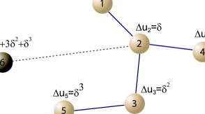
Figure 1: Schematic layout of network growth when $m=m_{0}=1$. The addition of a new node, $6$, implies an increase of the utility of nodes $1$ to $5$ which is simply $\delta^{d}$, where $d$ is the path length from node $6$. The simplicity of this updating mechanism allowed simulations to be run with $N=10^{5}$ when $m=1$.

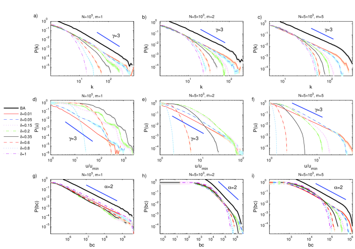
Figure 2: (Color online) Cumulative distribution function of degree (panels a), b) and c)), utility (panels d), e) and f)) and betweenness centrality (panels g), h) and i)) for several values of $\delta\in\left]0,1\right]$, and $m=1,2$ and $5$. We also plot the corresponding distribution of degree and betweenness for the BA model (curves were shifted vertically). Simulations were averaged over $30$ runs in networks with $N=10^{5}$ ($m=1$) or $N=5\times 10^{3}$ ($m=2$ and $5$). Coloured bands around the curves are $95\%$ confidence intervals.

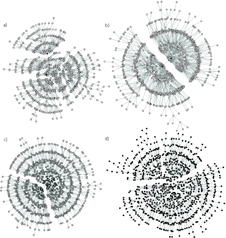
Figure 3: Kamada-Kawai spring layout Kamada89 for $m=1$ and $N=10^{3}$. Panel a) is a sample layout for $\delta=0.01$, b) for $\delta=0.2$, c) for $\delta=0.7$ and d) for $\delta=1$. On each panel, nodes are coloured by their utility on a gray scale from minimal (white) to maximal (black) utility.

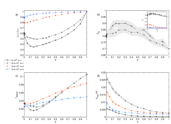
Figure 4: (Color online) Plots of a) average path length, b) central point dominance, c) assortativity coefficient, and d) normalized maximum degree as a function of $\delta$ for the simulation results when $m=1,2$ and $5$. Curves in panel a) were scaled by the values at $\delta=1$ (exponential network). The BA values are indicated by the corresponding full symbols. Simulations were averaged over $30$ runs and coloured bands around the curves are $95\%$ confidence intervals.

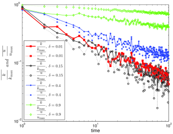
Figure 5: (Color online) Plots of average $k/k_{max}$ and $u/u_{max}$ as a function of the entry time for the first 100 nodes when $N=10^{5}$ and $m=1$. Simulations were averaged over $30$ runs.

In the classic Barabási and Albert model Barabasi99 , a network is grown by adding, at every time step, a new node that attaches to $m$ existing nodes with a probability proportional to their degree, $\Pi(k_{i})=k_{i}/\sum_{j=1}^{N}k_{j}$. At time $t$, the resulting network has size $N_{t}=m_{0}+t$, where $m_{0}\geq m$ is the size of the (fully connected) network at time $t=0$. Preferential attachment models were in fact introduced in the literature already by Yule Yule25 and Simon Simon55 .

The preferential attachment mechanism generates a scale-free probability density of incoming links that leads to the stationary result $p(k)=2m^{2}/k^{\gamma}$, with $\gamma=3$ independently of $m$. The model is also characterized by a clustering coefficient larger than the one found for the Erdős Rényi networks (for $m>1$) and no clear assortative/disassortative behaviour Albert02 .

Several models have been proposed lately to investigate extensions of the preferential attachment mechanism through edge removal and rewiring, inheritance, redirection or copying; node competition, aging and capacity constraints; and accelerated growth of networks to name just a few (see Albert02 ; Dorogovtsev02 ; NewmanSIAM03 ; Durrett07 for reviews).

Of particular relevance to our approach are fitness models Bedogne06 ; Caldarelli02 ; Masi06 ; Servedio04 , where the probability of attaching to a node is proportional to node fitness

$$\Pi(k_{i})\sim\frac{f_{i}k_{i}}{\sum_{j=1}^{N}f_{j}k_{j}}.$$ (4)

Here we extend the preferential attachment rule by introducing a growing mechanism inspired on the work of Jackson and Wolinsky Jackson96 . Our contribution is to propose preferential attachment by node utility. Thus, the probability that a new node $j$ will be connected to an existing node $i$ depends on the utility of $i$, such that

$$\Pi_{i}=\frac{u_{i}}{\sum_{k=1}^{N}u_{k}}$$ (5)

where the utility of node $i$, $u_{i}$, is given by (3). Attachment happens with uniform distribution for $\delta=1$ generating an exponential distribution of node degree . While the model is not defined for $\delta=0$, the preferential attachment rule (5) is invariant up to multiplicative factors in (3), so for $\delta\neq 0$ the qualitative behaviour of the model remains unchanged if we define utility as

$$u_{i}^{{}^{\prime}}=\frac{u_{i}}{\delta}=k_{i}+\sum_{l=2}^{l_{max}^{(i)}}\delta^{l-1}z_{l}^{(i)}$$ (6)

where $k_{i}$ is the degree of node $i$. Thus, as $\delta\rightarrow 0$ our model converges to the Barabási-Albert model and generates a scale-free network.

Our model has resemblances with the fitness models discussed above. However, there is a fundamental discrepancy: we regard utility as a time-dependent measure of node fitness, whereas existing models assume that node fitness does not change with time.

At each time step, a new node $j$ joins the network and the utility of existing nodes changes. When $m=1$, the utility increment to an existing node $i$ at distance $l$ from $j$ is given by $\Delta u_{i}=\delta^{l}$ and therefore, at each time step, the computation of utility for the network can be completed in $O(N)$ time. Figure 1 is a diagram of a possible network configuration with $m=m_{0}=1$ after $t=5$ time steps, showing the change in utility of existing nodes, $\Delta u_{i}=\delta^{l}$. When $m>1$, the increment in the utility of node $i$ depends on the existing network geometry and $\Delta u_{i}\geq\delta^{l}$. Therefore, when $m>1$, we need to re-compute the utility of all existing nodes at every time step, and the computation runs in $O(N^{2})$ time as it involves running a breadth-first-search algorithm from every node. This is the reason why we have ran simulations for $N=10^{5}$ when $m=1$, but only up to $N=5\times 10^{3}$ when $m>1$.

Existing nodes $i$ at a higher distance than a certain $l_{\max}$ from new node $j$ receive a contribution $\Delta u_{i}=\delta^{d(j,i)}<10^{-precison}$ which is less than the number of significant digits that the computer can store (typically $precison=32$ in double precision), and do not need to have their utility updated in the simulations. This maximal distance $l_{\max}$ is defined as

$$10^{-precision}>\delta^{l_{\max}}\Leftrightarrow l_{\max}>-\frac{precision}{\log_{10}\delta}$$ (7)

Our implementation of the algorithm updates the utility of all nodes accessible from the new node $j$ up to distance $l_{\max}=-32/\log_{10}\delta$. The code was implemented in C++ and ran on a Condor framework (high throughput computing) Thain05 for several values of $\delta$. Ensemble averages were taken over $30$ runs.

Expressions (3) and (6) predict the existence of two distinct regimes: a scale-free regime as $\delta\rightarrow 0$ ($\delta\neq 0$) and a random growth regime for which degree distribution is exponential at $\delta=1$. We are interested in exploring how the network evolves from one limit regime to the other as we increase $\delta$.

Figure 2a-c) shows the distribution of degree for $m=1,2$ and $5$. We also plot the corresponding distribution for the BA model (solid curves shifted vertically). For very small $\delta\sim 0.01$, preferential attachment by degree is indistinguishable from preferential attachment by utility and the probability distribution of both quantities decay like $p\left(x\right)\sim x^{-\gamma}$ with $\gamma=3$. The power-law decay in the BA model is known to be a peculiarity of the linear preferential attachment mechanism and is destroyed by small perturbations like, for example, a non-linear attachment rule $\Pi(k_{i})\sim k_{i}^{\alpha}$ Barabasi99 . Here we also observe a depart from the scale-free regime as we increase $\delta$. Furthermore, in the Barabási-Albert model the degree distribution decays as a power-law with exponent $\gamma=3$ independently of $m$. In our model, increasing $m$ has the effect of homogenizing the utility of the nodes (the distance between pairs of nodes decreases with increasing connectivity in the networks). Consequently, deviations from the power-law decay are observed at lower and lower values of $\delta$ as we increase $m$.

Betweenness centrality is plot in Figure 2g-i) as $m$ is varied. Recent results have shown that the distribution of loads (or betweenness) scales with a power law Goh01 ; Barthelemy04 $p(g)\sim g^{-\alpha}$ where $\alpha=2$ for a tree (and hence for $m=1$). This justifies the collapse of the curves of the distribution of betweenness in Figure 2g). As can be observed in Figure 2h) and i), the distribution of betweenness deviates from the power-law behaviour as $m$ is increased.

For intermediate values of $\delta$ and $m=1$ a number of interesting features appear. First of all, we observe that the utility distribution becomes step-like (Figure 2d) suggesting the presence of subsets of nodes that share similar utilities.

This phenomenon can also be inferred from the network layouts in Figure 3 (for networks of $10^{3}$ nodes with $m=1$), which are produced using the Kamada-Kawai spring layout Kamada89 . Essentially, the Kamada-Kawai layout assigns stronger springs to vertices that are closer in the graph-theoretic sense (i.e., by following edges) and therefore places them closer together. In the case $m=1$ (a tree), nodes close to the hubs on the graph layout will also be close in graph terms and therefore we can interpret the layout heuristically: these nodes have similar utility. When $\delta=0.01$ (close to the BA scale-free regime), the layout shows a few utility hubs (the dark vertices) surrounded by clouds of nodes that disperse as we move further away from the hubs; for $\delta=0.2$ denser clouds of nodes cluster around a smaller number of hubs, and can still be observed farther away from the hub; for higher $\delta$ the clouds start dispersing; eventually for $\delta=1$ all nodes have the same utility.

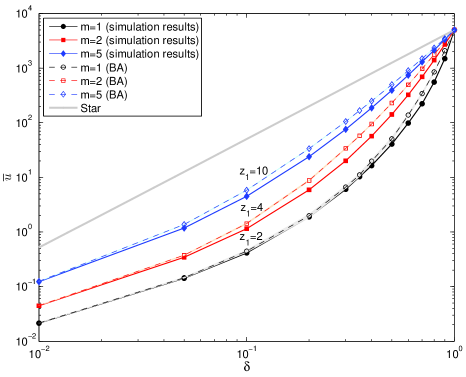
Figure 6: (Color online) Average utility for the simulation results (solid curve and symbols) and the BA model (dashed curve, open symbols) for $m=1$ ($z_{1}=2$), $2$ ($z_{1}=4$) and $5$ ($z_{1}=10$) when $N=5\times 10^{3}$. We also plot the average utility of a star with $N=5\times 10^{3}$ nodes. Simulation results were averaged over $30$ runs. Coloured bands around the curves are $95\%$ confidence intervals.

The rearrangement of the network as $\delta$ increases from zero gives rise to non monotonous behaviour of the average path length $\bar{l}$, degree assortativity $r_{degree}$ NewmanPRE03 , and central point dominance $C_{B}^{\prime}$ FreemanSociometry77 . Both $\bar{l}$ and $r_{degree}$ show a minimum for $\delta\sim 0.15$ ($N=10^{5}$ and $m=1$) and $C_{B}^{\prime}$ has a maximum around the same value. This behaviour can be observed in Figure 4a-c). The average path length $\overline{l}(\delta)$ is measured relative to the path length of a random growing network (i.e. relative to $\overline{l}(1)$). The scale-free regime is characterised by a shorter path length than the random growth regime. Here we observe an even further contraction of the network for values of $\delta$ up to $\sim 0.5$. Note that the average path length of a star network is $l^{\ast}=2$ for $N$ large. When normalizing with $l(1)=20.16$ we get a value of $l^{\ast}\sim 0.1$. While this value is still much smaller than $\overline{l}(0.15)$, the network contraction seems to indicate a move toward a more star-like configuration. To further investigate this point, we compute the the central point dominance measure introduced by Freeman FreemanSociometry77 and plot it in Figure 4b). This measure is defined as the average difference in node centrality (measured by node total betweenness) between the most central point and all the others. The central point dominance takes a value between zero (for a graph where all points have the same centrality) and one (for the wheel or star graph). The maximum of $C_{B}^{\prime}$ for $\delta\sim 0.15$ in Figure 4b) confirms that the network is becoming more star like around these values of $\delta$.

Next, we plot the assortativity of the network in Figure 4c). We implement as measure of assortativity the degree assortativity $r_{degree}$ NewmanPRE03 which takes values from $-1$ to $+1$: negative values for disassortative networks, $0$ if the networks are neither dissasortative or assortative, and $+1$ for fully assortative networks. This value approaches zero for large $N$ in the BA model NewmanPRL02 and is negative for a star. Our model shows a lower assortative mixing than the BA model for values of $\delta$ up to $\sim 0.5$. The decrease in $r_{degree}$ is also consistent with our hypothesis that the network is becoming more star like at $\delta\sim 0.15$. While the network goes through this rearrangement the degree of the most connected node (as a fraction of the total number of links) is nonetheless monotonously decreasing with $\delta$, as shown in Figure 4d). The same behaviour is observed for the utility of the most connected node (not shown here). This reveals that as new nodes are added to the network, they do attach on average closer to the hubs as $\delta$ increases, generating a more compact network, but not directly to them.

To gain further insights into the structural changes that take place as $\delta$ increases from zero, we analyze the role of entry time on node connectivity by computing the ratios $u/u_{max}$ and $k/k_{max}$ for the first $100$ nodes as a function of the time at which they entered the network. The ratios plotted in Figure 5 are averaged over 30 different simulations, for networks with $N=10^{5}$ and $m=1$. The plot shows that for any $\delta$ the initial node is likely to acquire the highest fraction of links and utility. Moreover, for $\delta=0.15$ both the degree and utility ratios decay faster than in the scale-free regime. This reveals that, for $\delta\sim 0.15$, the earlier nodes receive both a higher relative degree and utility than in the scale-free case. In other words, the earlier nodes are stronger hubs than in the scale-free case and thus the network arranges in a more star like configuration around $\delta=0.15$. As $\delta$ increases further, the slope of the utility ratio becomes lower than in the scale-free regime. In this range, the utility differences between old and new nodes are not large enough to create well defined utility or degree hubs.

Figure 5 also highlights the fundamental mechanism of structure formation in our model: the fine relation between degree and utility as $\delta$ is varied. In the scale-free regime, preferential attachment by utility is equivalent to preferential attachment by degree and node degree and utility assume the same value as the network grows. At $\delta\sim 0.15$, we observe a gap between the two scaled quantities, suggesting a discrepancy between degree and utility for the higher order neighbours of the utility hubs. This gap is larger for $\delta=0.15$ than $\delta=0.4$, indicating that around $\delta\sim 0.15$ the growth mechanism is generated by a variable (node utility) which is considerably independent of node degree and thus revealing why this is the region where the network displays more interesting structure. As $\delta$ increases towards $1$, the influence of random network growth becomes more important and this structure generating mechanism disappears.

Finally, we investigate how average node utility compares in networks generated with our preferential utility attachment, the scale-free regime (here generated via the BA preferential attachment mechanism) and a star network. The average utility of a star network is given by:

$$\overline{u}_{\ast}\left(\delta\right)=\delta z_{1}\left(1+\delta\frac{N-2}{2}\right)$$ (8)

where $z_{1}=2(N-1)/N$. For $N$ large, $z_{1}\simeq 2$ and $\overline{u}_{\ast}\left(\delta\right)\sim N\delta^{2}$. In Figure 6 we plot the average utility for networks in our model at different $\delta$ when $N=5\times 10^{3}$ and $z_{1}=2$, $4$ and $10$ and compare that to the corresponding average utility in the BA model and a star with the same $N$. The plot shows that the BA scale-free network has a higher utility than the network generated via our preferential utility mechanism at all values of delta and $z_{1}$. Networks in our model become more star-like for $\delta\sim 0.5$, but this implies an increase in the utility of only a small number of nodes (the early nodes). Therefore, the average utility of nodes in the network is still higher in the BA model than in our model for the same values of $\delta$ due to the scale-free structure of the former. Comparisons with the star network can only be made when $z_{1}=2$ as this is the average degree of the star network when $N$ is large. Figure 6 confirms that the star network has the highest utility for this value of $z_{1}$ among all the networks we study. Nevertheless, the star network can only be achieved if agents are perfectly rational and have access to full information (in which case the attachment mechanism would be deterministic). This is rarely the case in real word situation, thus the comparison with the star is of little practical relevance.

III Analytical Results for Random Networks

An interesting question to ask (for example, from the point of view of the social planner) is how network topologies rank against each other and which network structure maximizes the total, or the average utility (networks that satisfy this condition are said to be efficient in economics). We show that it is possible to derive analytical results for the average utility in Poisson and power-law networks. By comparing average utility in different network topologies with the same size and the same average degree, we show that power-law networks are more efficient than Poisson random networks (even though less efficient than the star). The effect of costs on $\overline{u}\left(\delta\right)$ is a constant term for all networks with the same $N$ and $z_{1}$. Therefore, without loss of generality, we choose $c=0$ in the analysis below.

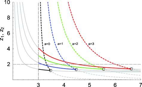
Figure 7: (Color online) Average number of first and second-neighbours ($z_{1}\left(\gamma,a\right)$ and $z_{2}\left(\gamma,a\right)$) in networks with degre distribution given by (15). From left to right, we plot $z_{1}\left(\gamma,a\right)$ (full curves) and $z_{2}\left(\gamma,a\right)$ (dashed curves) for $a=0$ (black), $1$ (blue), $2$ (green) and $3$ (red). The values of $z_{1}\left(\gamma\leq 3,a\right)$ for which $z_{2}\left(\gamma,a\right)$ is not defined are plot in grey, as well as regions of the curves for which $z_{1}\left(\gamma,a\right)>z_{2}\left(\gamma,a\right)$. The circles denote the intersection of the two curves, $z_{1}\left(\gamma,a\right)$ and $z_{2}\left(\gamma,a\right)$, for each value of $a$.

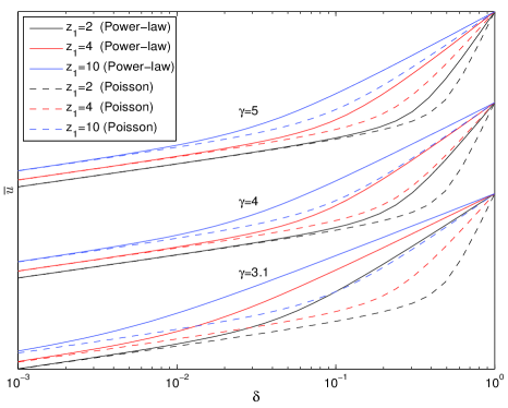
Figure 8: (Color online) Analytical results for average utility in networks with power-law (full curves) and Poisson (dashed curves) degree distributions as a function of $\delta$, $z_{1}$ and $\gamma$ for $N=10^{5}$. Curves have been shifted vertically for different values of $\gamma$ for clarity. Values of $z_{1}$ increase from bottom to top.

If the sum in (3) was to be evaluated up to distance $l_{max}^{(i)}=1$ for every node, expression (9) would simplify to $\overline{u}\left(\delta\right)=\delta z_{1}$, i.e. average utility would be independent of the specific network topology and all networks with the same number of nodes and links would be equally efficient. Thus we need to introduce long range interactions ($l_{max}^{(i)}>1$) to be able to rank networks in terms of their efficiency.

To derive an expression for average utility in generic random networks with $N$ large, we average both sides of (3):

$$\overline{u}\left(\delta\right)=\sum_{l=1}^{\overline{l}}\delta^{l}z_{l}$$ (9)

where $z_{l}$ is the average number of $l$th neighbours of a node. Newman et al. Newman01 ; Newman02 define $\overline{l}$ via the expression

$$1+\sum_{l=1}^{\overline{l}}z_{l}=N$$ (10)

Now that we have expressed average utility in terms of the breadth-first search algorithm, we can derive a closed form of expression (9) if we have access to analytical expressions for $\overline{l}$ and $z_{l}$. This can be accomplished by generating functions, which are particularly useful when determining means, standard deviations and moments of distributions Wilf94 .

The average number of neighbours (average degree) and the average number of second neighbours of a node can be derived from the probability generating function of node degree, $G_{0}\left(x\right)=\sum_{k=0}^{\infty}p_{k}x^{k}$, as long as the degree distribution, $p_{k}$, is specified. The beauty of the generating function formalism is that one can derive $z_{l}$ as a function of $z_{1}$ and $z_{2}$ only Callaway00 ; Newman01 ; Newman02 :

$$z_{l}=\left[\frac{z_{2}}{z_{1}}\right]^{l-1}z_{1}$$ (11)

Replacing equation (11) in equation (9) yields

$$\overline{u}\left(\delta\right)=\delta z_{1}\sum_{l=1}^{\overline{l}}\left(\delta Z\right)^{l-1}=\frac{\delta z_{1}(\left(\delta Z\right)^{\overline{l}}-1)}{\delta Z-1}$$ (12)

where $Z=z_{2}/z_{1}$. For $Z>1$ and $N>z_{1}+1$, which are conditions satisfied by most networks, $\overline{l}$ can be calculated as a function of $N$, $z_{1}$ and $z_{2}$ from (10) and (11) as Newman01 :

$$\overline{l}=\frac{\ln[\left(N-1\right)\left(Z-1\right)/z_{1}+1]}{\ln\left(Z\right)}$$ (13)

In what follows, we investigate the behaviour of (12) for Poisson and power-law random networks.

Poisson random networks are characterized by $z_{1}=pN$ and $z_{2}=z_{1}^{2}$ Newman01 , thus (13) yields $\overline{l_{P}}=\ln(\frac{N(z_{1}-1)+1}{z_{1}})/\ln(z_{1})$. In this case, (12) becomes:

$$\overline{u}_{P}\left(N,\delta,z_{1}\right)=\frac{z_{1}\delta\left(\left(\delta z_{1}\right)^{\ln(N+\frac{1-N}{z_{1}})/\ln(z_{1})}-1\right)}{\delta z_{1}-1}$$ (14)

for $N>z_{1}+1$, $0<\delta\leq 1$ and $z_{1}>1$.

Next, we consider power-law networks with degree distribution of the form:

$$p_{k}\left(\gamma,a\right)=\frac{1}{\zeta\left(\gamma,1+a\right)}(a+k)^{-\gamma}\quad,a\geq 0$$ (15)

where the normalizing factor $\zeta\left(\gamma,a+1\right)=\sum_{k=1}^{\infty}(a+k)^{-\gamma}$ is the Hurwitz zeta function ($\gamma>1$). The generating function for the probability distribution is given by

$$G_{0}\left(x,\gamma,a\right)=\sum_{k=1}^{\infty}p_{k}x^{k}=\frac{x\Phi(x,\gamma,a+1)}{\zeta\left(\gamma,a+1\right)}$$ (16)

where $\Phi(x,\gamma,a)=\sum_{k=0}^{\infty}\frac{x^{k}}{(a+k)^{\gamma}}$ is the Lerch transcendent. For our purposes, only the first two derivatives of $\Phi(x,\gamma,a+1)$ with respect to $x$ are relevant as the average number of first and second-neighbours are given, respectively, by $z_{1}\left(\gamma,a\right)=\left.\frac{\partial G_{0}(x)}{\partial x}\right|_{x=1}$ and $z_{2}\left(\gamma,a\right)=\left.\frac{\partial^{2}G_{0}(x)}{\partial x^{2}}\right|_{x=1}$. Hence

$$z_{1}\left(\gamma,a\right) =\frac{\Phi(1,\gamma-1,a+1)-a\Phi(1,\gamma,a+1)}{\zeta(\gamma,a+1)}\quad,\gamma>2\wedge a\geq 0$$ (17)

$$z_{2}\left(\gamma,a\right) =\frac{\zeta(\gamma-1,a+1)}{\zeta(\gamma,a+1)}z_{1}\left(\gamma-1,a\right)-(a+1)z_{1}\left(\gamma,a\right)\quad,\gamma>3\wedge a\geq 0$$ (18)

Thus

$$Z\left(\gamma,a\right)=\frac{\zeta(\gamma-1,a+1)}{\zeta(\gamma,a+1)}\frac{z_{1}\left(\gamma-1,a\right)}{z_{1}\left(\gamma,a\right)}-a-1\quad,\gamma>3\wedge a\geq 0$$ (19)

Substituting (17) and (19) into (13), we find

$$\overline{l}_{SF}\left(N,\gamma,a\right)=\frac{\ln\left(-\frac{(a+2)(N-1)}{z_{1}(\gamma,a)}+\frac{z_{1}(\gamma-1,a)\zeta(\gamma-1,a+1)(N-1)}{z_{1}(\gamma,a)^{2}\zeta(\gamma,a+1)}+1\right)}{\ln\left(-a+\frac{z_{1}(\gamma-1,a)\zeta(\gamma-1,a+1)}{z_{1}(\gamma,a)\zeta(\gamma,a+1)}-1\right)}\quad,N>z_{1}\left(\gamma,a\right)+1\wedge\gamma>3\wedge a\geq 0\wedge Z\left(\gamma,a\right)>1$$ (20)

and thus average utility is given by

$$\overline{u}_{SF}\left(N,\delta,\gamma,a\right)=\frac{\delta z_{1}\left(\gamma,a\right)\left(\left(\delta Z\left(\gamma,a\right)\right)^{\overline{l}_{SF}\left(N,\gamma,a\right)}-1\right)}{\delta Z\left(\gamma,a\right)-1}\quad,N>z_{1}\left(\gamma,a\right)+1\wedge 0<\delta\leq 1\wedge\gamma>3\wedge a\geq 0\wedge Z\left(\gamma,a\right)>1$$ (21)

where $z_{1}\left(\gamma,a\right)$, $Z\left(\gamma,a\right)$ and $\overline{l_{SF}}\left(N,\gamma,a\right)$ are given by (17), (19) and (20), respectively.

When $a=0$, the distribution of degree, (15), becomes a pure power-law $p_{k}\left(\gamma\right)=\frac{1}{\zeta\left(\gamma\right)}k^{-\gamma}$. In this case, we have $\left.\zeta\left(\gamma,a+1\right)\right|_{a=0}=\zeta\left(\gamma\right)$ and $\left.\Phi(x,\gamma,a+1)\right|_{a=0}=\frac{Li_{\gamma}\left(x\right)}{x}$, therefore (16) becomes

$$G_{0}\left(x,\gamma\right)=\frac{\text{Li}_{\gamma}\left(x\right)}{\zeta\left(\gamma\right)}$$ (22)

This generating function is also obtained for the power-law distribution with exponential cut-off, proposed in Aldana03 ; NewmanPRL05 , $p_{k}\left(\gamma,\kappa\right)=Ck^{-\gamma}e^{-k/\kappa}$, in the limit $\kappa\rightarrow\infty$.

Expression (22) implies

$$\left.z_{1}\left(\gamma\right)\right|_{a=0}=\frac{\zeta\left(\gamma-1\right)}{\zeta\left(\gamma\right)}\quad,\gamma>2$$ (23)

$$\left.z_{2}\left(\gamma\right)\right|_{a=0}=\frac{\zeta\left(\gamma-2\right)-\zeta\left(\gamma-1\right)}{\zeta\left(\gamma\right)}\quad,\gamma>3$$ (24)

Therefore, in pure power-law networks, when $N\rightarrow\infty$, the average number of second-neighbours, $z_{2}\left(\gamma\right)$, is finite only for $\gamma>3$. However, the Riemann zeta function, $\zeta\left(\gamma\right)$, is a decreasing function of $\gamma$ (for $\gamma>3$) and $z_{1}\left(\gamma=3\right)=\pi^{2}/6\zeta(3)\simeq 1.36843$. In other words, the existence of $z_{2}\left(\gamma\right)$ implies $z_{1}\left(\gamma\right)<z_{1}\left(\gamma=3\right)\simeq 1.36843$, which is a non-realistically low value for average degree in real networks. This explains why we have chosen the modified power-law distribution (15).

The generating function (16) encapsulates all the moments of the degree distribution Newman01 . Hence, the expressions for $z_{1}\left(\gamma,a\right)$ and $z_{2}\left(\gamma,a\right)$, (17) and (18), are only exact in the limit $N\rightarrow\infty$. Further, $\overline{l}_{SF}\left(N,\gamma,a\right)$ and $\overline{u}_{SF}\left(N,\delta,\gamma,a\right)$, both of which depend on $z_{2}\left(\gamma,a\right)$, are only defined where $z_{2}\left(\gamma,a\right)$ is finite, i.e. for $\gamma>3$. Therefore, it is essential to understand the behaviour of $z_{1}\left(\gamma,a\right)$ and $z_{2}\left(\gamma,a\right)$ in power-law networks. Figure 7 shows $z_{1}$ (full curves) and $z_{2}$ (dashed curves) within the range $\gamma>3\wedge Z>1$ (where $\overline{l}_{SF}\left(N,\gamma,a\right)$ is defined) for, from left to right, $a=0,1,2$ and $3$.

Having deduced closed-form expressions for average utility in Poisson and power-law networks, we can now compare both networks under the condition that $z_{1}$ is the same. Figure 8 is a plot of average utility versus $\delta$ when $z_{1}=\left\{2,4,10\right\}$ and $N=10^{5}$ for Poisson and power-law networks. The average utility of Poisson networks is completely specified by $N,\delta$ and $z_{1}$, but power-law networks defined by (15) have one extra degree of freedom in $z_{1}\left(\gamma,a\right)$. In this case, we compute $z_{1}$ numerically by solving (17) for $z_{1}\left(\gamma,a\right)=\left\{2,4,10\right\}$ when $\gamma=\left\{3.1,4,5\right\}$. For all cases studied power-law networks are more efficient than Poisson networks.

IV Discussion

The growth mechanism we have proposed is a natural extension of the Barabási-Albert preferential attachment by degree to preferential attachment by node utility. Our analysis shows that for small values of $\delta$, the utility decay parameter, the network retains a scale-free structure that is nonetheless destroyed when $\delta$ increases. We have identified a regime in $\delta$ where the network is characterized by a lower average path length and assortativity coefficient and a higher central point dominance than the scale-free network. In this regime, the distribution of utility is a step-like function and the network has a more star-like structure.

The derivation of analytical expressions for average utility in Poisson and power-law networks reveals that the latter have higher $\overline{u}$ for the range of parameters that is of significance in real-world networks ($z_{1}\geq 2$). This suggests a novel mechanism which may explain the ubiquitous presence of power-law networks, in particular in situations where collaboration, interaction and information sharing among the nodes are of paramount relevance.

Social networks are highly volatile. Friendships can be stable for a long time but occasional encounters may lead to creation of links that are never used again in the future. A dynamical model of network formation, where links not only can be heterogenous, but whose weights can change continuously over time, would be a more appropriate way to describe social interactions. Our assumption that $w_{ij}=1$ for all links is obviously a first order approximation and preferential growth, with no link rearrangements, is a crude description of social network formation. Nonetheless even this simple mechanism can highlight surprising features of the models (like in our case a smaller network diameter for intermediate values of $\delta$) and as such it is worth to investigate in more general contests than the original BA model.

We have also assumed that the connection costs in our model are zero. This assumption is justified by the fact that if costs are node independent they do not play any role in the growing model. Similarly, costs do not play a significative role if we restrict the comparison of average utility in section III to networks with the same size and the same average degree. Nonetheless in a more realistic model, where links can be rearranged over time, costs would also play an important role in determining the shape of the network.

Further analysis taking into account both these effects is currently under development.

- (1) M. O. Jackson and A. Wolinsky, Journal of Economic Theory 71, 44 (1996).
- (2) V. Bala and S. Goyal, Econometrica 68, 1181 (2000).
- (3) M. Marsili, F. Vega-Redondo, and F. Slanina, Proceedings of the National Academy of Sciences U.S.A. 101, 1439 (2004).
- (4) D. O. Cajueiro, Physical Review E 72, 047104 (2005).
- (5) G. C. M. A. Ehrhardt, M. Marsili, and F. Vega-Redondo, Physical Review E 74, 036106 (2006).
- (6) A. D. Martino and M. Marsili, Journal of Physics A: Mathematical and General 39, R465 (2006).
- (7) G. Iori, S. Jafarey, and F. G. Padilla, Journal of Economic Behaviour and Organization 61, 525 (2006).
- (8) M. O. Jackson, The economics of social networks, in Advances in Economics and Econometrics, Theory and Applications: Ninth World Congress of the Econometric Society, edited by W. N. Richard Blundell and T. Persson, volume I, Cambridge University Press, 2006.
- (9) R. Albert and A.-L. Barabási, Reviews of Modern Physics 74, 47 (2002).
- (10) M. Newman, SIAM Review 45, 167 (2003).
- (11) S. N. Dorogovtsev and J. F. F. Mendes, Evolution of Networks: From Biological Nets to the Internet and WWW, Oxford University Press, 2003.
- (12) A.-L. Barabási and R. Albert, Science 286, 509 (1999).
- (13) F. Feri, Journal of Economic Theory (2007, forthcoming).
- (14) J. Kleinberg and E. Tardos, Algorithm Design, Addison Wesley, 2006.
- (15) H. S. Wilf, Generatingfunctionology, Academic Press, 1994.
- (16) T. Kamada and S. Kawai, Information Processing Letters 31, 7 (1989).
- (17) S. N. Dorogovtsev and J. F. F. Mendes, Advances in Physics 51, 1079 (2002).
- (18) C. Bedogne and G. J. Rodgers, Physical Review E 74, 046115 (2006).
- (19) G. Caldarelli, A. Capocci, P. D. L. Rios, and M. A. Munõz, Physical Review Letters 89, 258702 (2002).
- (20) G. D. Masi, G. Iori, and G. Caldarelli, 74, 066112 (2006).
- (21) V. D. P. Servedio, G. Caldarelli, and P. Buttà, Physical Review E 70, 056126 (2004).
- (22) D. Thain, T. Tannenbaum, and M. Livny, Concurrency and Computation: Practice and Experience 17, 323 (2005).
- (23) K.-I. Goh, B. Kahng, and D. Kim, Physical Review Letters 87, 278701 (2001).
- (24) M. Barthélemy, Eur. Phys. J. B 38, 163 (2004).
- (25) M. E. J. Newman, Physical Review E 67, 026126 (2003).
- (26) L. C. Freeman, Sociometry 40, 35 (1977).
- (27) M. E. J. Newman, Phys. Rev. Lett. 89, 208701 (2002).
- (28) M. E. J. Newman, S. H. Strogatz, and D. J. Watts, Physical Review E 64, 026118 (2001).
- (29) M. Newman, D. J. Watts, and S. H. Strogatz, Proceedings of the National Academy of Sciences U.S.A. 99, 2566 (2002).
- (30) D. S. Callaway, M. E. J. Newman, S. H. Strogatz, and D. J. Watts, Physical Review Letters 85, 5468 (2000).
- (31) M. Aldana, Physica D 185, 45 (2003).
- (32) M. E. J. Newman, Physical Review Letters 95, 108701 (2005).
- (33) G. U. Yule Phil. Trans. R. Soc. Lond. B 213, 21 (1925).
- (34) H. A. Simon Biometrika 42, 425 (1955) .
- (35) R. Durrett Random graph dynamics, Cambridge University Press, 2007