Semi-Lorentz invariance, unitarity, and critical exponents of symplectic fermion models

Abstract

We study a model of $N$-component complex fermions with a kinetic term that is second order in derivatives. This symplectic fermion model has an $Sp(2N)$ symmetry, which for any $N$ contains an $SO(3)$ subgroup that can be identified with rotational spin of spin-${1\over 2}$ particles. Since the spin-${1\over 2}$ representation is not promoted to a representation of the Lorentz group, the model is not fully Lorentz invariant, although it has a relativistic dispersion relation. The hamiltonian is pseudo-hermitian, $H^{\dagger}=CHC$, which implies it has a unitary time evolution. Renormalization-group analysis shows the model has a low-energy fixed point that is a fermionic version of the Wilson-Fisher fixed points. The critical exponents are computed to two-loop order. Possible applications to condensed matter physics in $3$ space-time dimensions are discussed.

I Introduction

A basic result in the quantum field theory of fundamental particles in $4$ space-time dimensions is that requiring Lorentz invariance for spin-$\frac{1}{2}$ particles necessarily leads to the free Dirac lagrangian. Here “spin-$\frac{1}{2}$” refers to the 3-dimensional rotational subgroup of the Lorentz group. The Lie algebra of the Lorentz group is $SU(2)\otimes SU(2)$, where one linear combination of the two $SU(2)$ symmetries is identified as angular momentum; thus spin representations are promoted to Lorentz representations in a straightforward manner.

This paper in part deals with the following basic question. Suppose one wishes to describe the quantum field theory of spin-$\frac{1}{2}$ particles in a physical context where the dispersion relation happens to be Lorentz invariant, but unlike in fundamental particle physics the full Lorentz invariance is not evidently required. In particular, we have in mind systems in condensed matter physics where the relativistic dispersion relation arises as a consequence of special properties of the system, and what plays the role of the speed of light is some material-dependent velocity. For instance, the effective mass of electronic quasi-particles may go zero because one is near a quantum critical point or more simply because of band structure as in 2-dimensional graphene Geim ; Kim , and massless particles, like photons, usually require a relativistic dispersion relation. Under these circumstances, the question is whether such a quantum field theory must necessarily be that of a Dirac fermion. In the case of graphene, the fermionic quasi-particles do turn out to be described by the massless Dirac equation. The reason for this is not an intrinsic Lorentz invariance, but rather that the continuum limit of a tight binding model on a hexagonal lattice gives a hamiltonian that is first order in derivatives, and near the Fermi points the particles are massless.

In this paper we will study an alternative to the Dirac theory. The model is built out of an $N$-component complex fermionic field with a non-Dirac, two-derivative action with a Lorentz-invariant dispersion relation. This model has a symplectic $Sp(2N)$ symmetry. If this symmetry is viewed as an internal symmetry, then the fields are Lorentz scalars and the theory is Lorentz invariant but with the “wrong” statistics. However, since the Lie group $Sp(2N)$ has an $SO(3)$ subgroup, we can identify the latter with rotational spin. Therefore our model can naturally describe spin-$\frac{1}{2}$ particles. The fermionic statistics is then in accordance with the spin-statistics connection, which requires spin-$\frac{1}{2}$ particles to be described by fermionic fields. However since the rotational spin-$\frac{1}{2}$ is not promoted to a representation of the Lorentz group as in the Dirac theory, our model is strictly speaking not Lorentz invariant; hence the terminology “semi-Lorentz” invariant.

The most serious potential problem of this theory concerns its unitarity, and this is addressed in the present paper. We show that the hamiltonian is pseudo-hermitian,

$$H^{\dagger}=CHC\,,$$ (1)

where $C$ is a unitary operator satisfying $C^{2}=1$. This generalization of hermiticity was considered long ago by Pauli Pauli , and more recently by Mostafazadeh Mostafazadeh as a way of explaining the real spectrum and addressing the unitarity issue in ${\cal P}{\cal T}$ symmetric quantum mechanics Bender1 ; Bender2 . The important point is that by suitably defining a $C$-dependent inner product, pseudo-hermiticity of $H$ is sufficient to ensure a unitary (i.e., norm-preserving) time evolution. This is explained in section II. One should also point out that taking a non-relativistic limit in the kinetic term one obtains a perfectly unitary second-quantized description of interacting fermions.

The identification of the $SO(3)$ Lie sub-algebra of $Sp(2N)$ with rotational spin is described in section III. There we also study the discrete space-time symmetries of time-reversal and parity, and show how the spin generators transform properly under them.

Another possible signature of non-unitarity comes from studying finite-size or finite-temperature effects. We show in section IV that whereas imposing periodic boundary conditions leads to a negative coefficient in the free energy, correctly imposing anti-periodic boundary conditions, as is normally appropriate for fermions, leads to a positive coefficient. (In two dimensions this coefficient is related to the Virasoro central charge.)

Symplectic fermions are interesting for potential applications to critical phenomena. First of all, in $D=3$, since the group of spacial rotations is simply $U(1)$, there are less constraints coming from Lorentz invariance. More importantly, unlike Dirac fermions, four-fermion interactions in $D=3$ drive the theory to some novel low-energy fixed points that are fermionic versions of the Wilson-Fisher WilsonFisher fixed points. The reason is simple: in three dimensions a symplectic fermion $\chi$ has classical (or mean field) scaling dimension $1/2$, whereas Dirac fermions $\psi$ have dimension 1; therefore $\chi^{4}$ is a dimension-2 operator and is relevant in $D=3$, whereas $\psi^{4}$ is irrelevant. This was the original motivation for the work spinon , where it was attempted to interpret these fixed points at $N=2$ as examples of deconfined quantum criticality Senthil . Although it remains unclear whether our fermionic critical point can correctly describe deconfined quantum criticality as defined in Senthil , the resolution of the unitarity problem as presented in this paper is sufficient motivation to analyze the critical exponents further. In sections V and VI we extend the analysis of spinon to two-loop order. In particular, we show that some of the critical exponents can be obtained by analytically continuing known results for the $O(M)$ Wilson-Fisher fixed point to $M=-2N$ . We also calculate the critical exponents for composite bilinear operators, which to our knowledge have not been studied for the $O(M)$ fixed points .

The correspondence of our model with $O(M)$ for negative $M$ is merely formal and not expected to be valid for all physical properties. First of all, the symmetries of the models are different. It should also be clear from the fact that in applications to condensed matter physics, our model has a Fermi surface, etc. Some concrete distinctions in the finite-size effects are made in section IV.

In section VII we speculate on some possible applications to $2+1$ dimensional quantum criticality in condensed matter physics. In the broadest terms, at the fixed point our model can be viewed as a quantum critical theory of spinons, where the symplectic fermions are fundamental spinon fields. For $N=2$ components, we discuss possible applications to quantum anti-ferromagnetism, where the magnetic order parameter ${\vec{n}}$ is a composite operator in terms of spinons ${\vec{n}}=\chi^{\dagger}\vec{\sigma}\,\chi$. This compositeness is the same as in deconfined quantum criticality Senthil , however our model is different since it has no $U(1)$ gauge field. We show that two-point correlation exponents ($\eta$) are rather large compared to the bosonic Wilson-Fisher fixed point, and this is mainly due to the compositeness of ${\vec{n}}$. By treating both cases, we show this is true irrespective of whether the particles are bosons or fermions.

Section VIII contains a summary of our main findings and some conclusions.

II Pseudo-hermiticity and unitarity of complex scalar fermions

Let $\chi$ denote an $N$-component complex field and consider the following action in $D=d+1$ dimensional Minkowski space:

$$S_{\chi}=\int d^{d}{\bf x}\,dt\left[\partial^{\mu}{\overline{\chi}}\partial_{\mu}\chi-m^{2}\,{\overline{\chi}}\chi-4\pi^{2}g\,({\overline{\chi}}\chi)^{2}\right],$$ (2)

where ${\overline{\chi}}\chi=\sum_{\alpha=1}^{N}{\overline{\chi}}^{\alpha}\chi^{\alpha}$, and $\partial^{\mu}\partial_{\mu}=\partial_{t}^{2}-\partial_{\bf x}^{2}$. If $\chi$ is taken to be a Lorentz scalar, then the model is Lorentz invariant. The above action has an explicit internal $U(N)$ symmetry. In the next section we show that, if $\chi$ is a fermion, then there is actually a hidden $Sp(2N)$ symmetry.

We wish to quantize this model with $\chi$ taken to be a fermionic (Grassman) field. The conjugate-momentum fields are $\pi_{\chi}=-\partial_{t}{\overline{\chi}}$ and $\pi_{\overline{\chi}}=\partial_{t}\chi$. They obey the canonical anti-commutation relations

$$\{{\overline{\chi}}^{\alpha}({\bf x},t),\partial_{t}\chi^{\beta}({\bf x}^{\prime},t)\}=-\{\chi^{\alpha}({\bf x},t),\partial_{t}{\overline{\chi}}^{\beta}({\bf x}^{\prime},t)\}=i\delta^{\alpha\beta}\delta^{(d)}({\bf x}-{\bf x}^{\prime})\,.$$ (3)

The hamiltonian for this system is

$$H=\int d^{d}{\bf x}\left[\partial_{t}{\overline{\chi}}\partial_{t}\chi+\partial_{\bf x}{\overline{\chi}}\partial_{\bf x}\chi+m^{2}\,{\overline{\chi}}\chi+4\pi^{2}g\,({\overline{\chi}}\chi)^{2}\right].$$ (4)

Note that because of the fermion statistics the interaction term vanishes for $N=1$.

Consider first the free theory with $g=0$. Suppressing the component indices, the fields have the following mode expansions consistent with the equations of motion:

$$\chi(x) = \int\frac{d^{d}{\bf k}}{(2\pi)^{d/2}\sqrt{2\omega_{\bf k}}}\left(b_{{\bf k},-}^{\dagger}\,e^{-ik\cdot x}+b_{{\bf k},+}\,e^{ik\cdot x}\right),$$

$${\overline{\chi}}(x) = \int\frac{d^{d}{\bf k}}{(2\pi)^{d/2}\sqrt{2\omega_{\bf k}}}\left(-b_{{\bf k},-}\,e^{ik\cdot x}+b_{{\bf k},+}^{\dagger}\,e^{-ik\cdot x}\right),$$ (5)

where $\omega_{\bf k}=\sqrt{{\bf k}^{2}+m^{2}}$ and $k\cdot x=\omega_{\bf k}\,t-{\bf k}\cdot{\bf x}$. The extra minus sign in the $b_{-}$ term in ${\overline{\chi}}$ is chosen so that the anti-commutation relations (3) lead to the standard non-vanishing canonical relations

$$\{b_{{\bf k}+},b^{\dagger}_{{\bf k}^{\prime}+}\}=\{b_{{\bf k}-},b^{\dagger}_{{\bf k}^{\prime}-}\}=\delta^{(d)}({\bf k}-{\bf k}^{\prime})\,,$$ (6)

where it is understood that the field operators belong to the same field component. Of course, the extra sign would be unnecessary if $\chi$ was a bosonic field.

With the above definitions the fields have the required properties under causality (see for instance Weinberg ), namely $\{\chi^{\alpha}(x),\chi^{\beta}(y)\}=\{{\overline{\chi}}^{\alpha}(x),{\overline{\chi}}^{\beta}(y)\}=0$ and

$$\{\chi^{\alpha}(x),{\overline{\chi}}^{\beta}(y)\}=\delta^{\alpha\beta}\left[\Delta_{+}(x-y)-\Delta_{+}(y-x)\right],$$ (7)

where

$$\Delta_{+}(x)=\int\frac{d^{d}{\bf k}}{(2\pi)^{d}\,2\omega_{\bf k}}\,e^{i{\bf k}\cdot{\bf x}}\,.$$ (8)

Since $\Delta_{+}(x)$ depends only on $x^{2}$ and is well-defined for space-like separation ($x^{2}<0$), it follows that $\chi(x)$ and ${\overline{\chi}}(y)$ anti-commute for space-like separated points $x$ and $y$. This implies that the hamiltonian densities ${\cal H}(x)$ and ${\cal H}(y)$ also commute at space-like separation. We will return to the spin-statistics connection below.

In terms of the momentum-space modes, the free hamiltonian is

$$H=\int d^{d}{\bf k}~{}\omega_{\bf k}\left(b^{\dagger}_{{\bf k}+}b_{{\bf k}+}-b_{{\bf k}-}b^{\dagger}_{{\bf k}-}\right)=\int d^{d}{\bf k}~{}\omega_{\bf k}\left(b^{\dagger}_{{\bf k}+}b_{{\bf k}+}+b^{\dagger}_{{\bf k}-}b_{{\bf k}-}\right)+\mbox{const.}$$ (9)

We can discard the infinite constant in the above equation, which is equivalent to normal-ordering the hamiltonian. Let us define the vacuum $|0\rangle$ as the state being annihilated by $b_{\pm}$. As a result, all states have positive energy. The one-particle states are doubly degenerate:

$$H\,b^{\dagger}_{{\bf k},\pm}|0\rangle=H|{\bf k},\pm\rangle=\omega_{\bf k}|{\bf k},\pm\rangle\,.$$ (10)

For $N=1$ the theory is manifestly invariant under a $U(1)$ symmetry. The corresponding conserved current satisfying $\partial^{\mu}J_{\mu}=0$ is $J_{\mu}=i[(\partial_{\mu}{\overline{\chi}})\chi-{\overline{\chi}}\,\partial_{\mu}\chi]$. The conserved charge $Q=\int d^{d}{\bf x}\,J_{t}({\bf x})$ can be expressed as

$$Q=\int d^{d}{\bf k}~{}\omega_{\bf k}\left(b^{\dagger}_{{\bf k}+}b_{{\bf k}+}+b_{{\bf k}-}b^{\dagger}_{{\bf k}-}\right).$$ (11)

With these conventions, the operators $b^{\dagger}_{+}$ and $b_{-}$ have charge $Q=1$, whereas $b^{\dagger}_{-}$ and $b_{+}$ have charge $Q=-1$.

The usual spin-statistics connection (see for instance Weinberg ) is based on causality as described above, along with the requirement that the hamiltonian must be constructed out of $\chi$ and its hermitian adjoint in order for it to be hermitian. The latter is violated here: because of the extra minus sign in the mode expansion of ${\overline{\chi}}$ for the fermionic case, one sees that unlike for the bosonic case, ${\overline{\chi}}$ is not the hermitian adjoint of $\chi$. Let us introduce a unitary operator $C$ satisfying $C^{\dagger}C=1$ and $C=C^{\dagger}$, which is defined by the properties $Cb_{\pm}C=\pm b_{\pm}$ and $Cb_{\pm}^{\dagger}C=\pm b_{\pm}^{\dagger}$. Then the relation between ${\overline{\chi}}$ and $\chi$ can be expressed as

$${\overline{\chi}}=C\chi^{\dagger}C\,.$$ (12)

Since $({\overline{\chi}}\chi)^{\dagger}=C{\overline{\chi}}\chi C$, the hamiltonian satisfies the “intertwined” hermiticity condition

$$H^{\dagger}=CHC\,.$$ (13)

The above is also true in the interacting theory since $[({\overline{\chi}}\chi)^{2}]^{\dagger}=C({\overline{\chi}}\chi)^{2}C$. (Note that for the free theory in momentum space, $C$ actually commutes with $H$ as can be seen from eq. (9), and hence the above equation is trivially satisfied; however, this is no longer the case in the interacting theory.)

Hamiltonians satisfying eq. (13) were considered long ago by Pauli Pauli and more recently by Mostafazadeh Mostafazadeh in connection with ${\cal P}{\cal T}$ symmetric quantum mechanics Bender1 ; Bender2 . We will follow the previously introduced terminology and refer to such hamiltonians as $C$-pseudo-hermitian. Quantum mechanics based on pseudo-hermitian operators has some very desirable properties, which parallel the standard ones. First of all, as we now explain, a pseudo-hermitian hamiltonian can still define a unitary quantum mechanics if one defines the inner product appropriately. Specifically, consider a new inner product defined as

$$\langle\psi^{\prime}|\psi\rangle_{c}\equiv\langle\psi^{\prime}|C|\psi\rangle\,.$$ (14)

Then probability is conserved with respect to this modified inner product, i.e., the norms of states are preserved under time evolution:

$$\langle\psi^{\prime}(t)|\psi(t)\rangle_{c}=\langle\psi^{\prime}|e^{iH^{\dagger}t}Ce^{-iHt}|\psi\rangle=\langle\psi^{\prime}|Ce^{iHt}C^{2}e^{-iHt}|\psi\rangle=\langle\psi^{\prime}|\psi\rangle_{c}\,.$$ (15)

Pseudo-hermiticity also ensures that the eigenvalues of $H$ are real. To see this, let $|\psi_{E}\rangle$ denote an eigenstate of $H$ with eigenvalue $E$. Then

$$(E-E^{*})\,\langle\psi_{E}|\psi_{E}\rangle_{c}=\langle\psi_{E}|(CH-H^{\dagger}C)|\psi_{E}\rangle=0\,.$$ (16)

Therefore eigenstates of $H$ with non-zero C-norm necessarily have real energies. Other properties are proven in Mostafazadeh .

In the sequel it will be convenient to define the pseudo-hermitian adjoint $A^{\dagger_{c}}$ of any operator $A$ as the proper hermitian adjoint with respect to the C-inner product:

$$\langle\psi^{\prime}|A|\psi\rangle_{c}^{*}\equiv\langle\psi|A^{\dagger_{c}}|\psi^{\prime}\rangle_{c}\,,$$ (17)

which implies

$$A^{\dagger_{c}}=CA^{\dagger}C\,.$$ (18)

The pseudo-hermiticity condition on the hamiltonian then simply reads $H^{\dagger_{c}}=H$. One can easily establish that this pseudo-hermitian adjoint satisfies the usual rules, e.g.

$$(AB)^{\dagger_{c}} = B^{\dagger_{c}}A^{\dagger_{c}}\,,$$

$$(aA+bB)^{\dagger_{c}} = a^{*}A^{\dagger_{c}}+b^{*}B^{\dagger_{c}}\,,$$ (19)

where $A,B$ are operators and $a,b$ are complex numbers.

III $Sp(2N)$ symmetry and rotational spin

The action (2) has an explicit $U(N)$ symmetry irrespective of whether $\chi$ is bosonic or fermionic. If $\chi$ is bosonic, then the action expressed in terms of real fields has an $O(2N)$ symmetry. On the other hand, if $\chi$ is a fermionic field, then the symmetry is $Sp(2N)$. Even for $N=1$, the $Sp(2)$ symmetry of the fermionic theory is larger than the $U(1)$ symmetry of the bosonic theory. To manifest this symmetry explicitly, let us express each component $\chi^{\alpha}$ as

$$\chi^{\alpha}={1\over\sqrt{2}}\,(\eta_{1}^{\alpha}+i\eta_{2}^{\alpha})\,,\qquad{\overline{\chi}}^{\alpha}=\frac{-i}{\sqrt{2}}\,(\eta_{1}^{\alpha}-i\eta_{2}^{\alpha})\,.$$ (20)

We now introduce the $2\times 2$ anti-symmetric matrix $\epsilon=\Big{(}\begin{array}[]{rc}0{}&1\\[-5.69046pt] -1{}&0\end{array}\Big{)}$ and the $2N\times 2N$ matrix $\epsilon_{N}=\epsilon\,\otimes 1_{N}$. Arranging the real fields $\eta_{i}^{\alpha}$ into a $2N$ vector $\eta=(\eta_{1}^{1},\eta_{2}^{1},\eta^{2}_{1},\eta^{2}_{2},\dots,\eta_{1}^{N},\eta_{2}^{N})$, one has

$${\overline{\chi}}\chi={1\over 2}\,\eta^{T}\epsilon_{N}\eta\,.$$ (21)

This bilinear form has the symmetry $\eta\to M\eta$, where $M^{T}\epsilon_{N}M=\epsilon_{N}$. This is the defining relation for $M$ to be an element of the group $Sp(2N)$.

We will need the Lie algebra of $Sp(2N)$. Let $M=e^{X}$, in which case the above relation implies $X^{T}\epsilon_{N}=-\epsilon_{N}X$. A linearly independent basis for $X$ is then $\{1\otimes A,\sigma_{x}\otimes t_{x},\sigma_{y}\otimes t_{y},\sigma_{z}\otimes t_{z}\}$, where $A$ is an $N\times N$ anti-symmetric matrix, $\sigma_{i}$ are the Pauli matrices, and $t_{i}$ are $N\times N$ symmetric matrices Georgi . For any $N$ the algebra $Sp(2N)$ has an $SO(3)$ sub-algebra generated by $\sigma_{i}\otimes 1_{N}$, which can in principle be identified with spin. It also has an $SO(N)$ sub-algebra generated by the matrices $A$, and an $SU(N)$ sub-algebra generated by $1\otimes A$ and $\sigma_{z}\otimes t_{z}$, where $t_{z}$ is traceless. The Lie algebra $Sp(2)$ is equivalent to $SO(3)\cong SU(2)$. Note that the $N=2$ case therefore has two different $SO(3)$ sub-algebras that could potentially be identified with spin.

III.1 Canonical quantization and pseudo-hermiticity

For simplicity, let us specialize to the free theory with $N=1$ component (the generalization to $N\neq 1$ is straightforward). Then the action takes the form

$$S=\int d^{d}{\bf x}\,dt\left(\partial^{\mu}\eta_{1}\partial_{\mu}\eta_{2}-m^{2}\eta_{1}\eta_{2}\right).$$ (22)

The canonical momenta are $\pi_{1}=\partial_{t}\eta_{2}$ and $\pi_{2}=-\partial_{t}\eta_{1}$, which leads to the equal-time anti-commutation relations

$$\{\eta_{1}({\bf x},t),\partial_{t}\eta_{2}({\bf x}^{\prime},t)\}=-\{\eta_{2}({\bf x},t),\partial_{t}\eta_{1}({\bf x}^{\prime},t)\}=i\delta^{(d)}({\bf x}-{\bf x}^{\prime})\,.$$ (23)

The pseudo-hermiticity of the hamiltonian exactly parallels the discussion in section II. If one expands the fields as

$$\eta_{1}(x) = \int\frac{d^{d}{\bf k}}{(2\pi)^{d/2}\sqrt{2\omega_{\bf k}}}\left(a_{{\bf k}+}^{\dagger}\,e^{-ik\cdot x}+a_{{\bf k}-}\,e^{ik\cdot x}\right),$$

$$\eta_{2}(x) = \int\frac{d^{d}{\bf k}}{(2\pi)^{d/2}\sqrt{2\omega_{\bf k}}}\left(-a_{{\bf k}-}^{\dagger}\,e^{-ik\cdot x}+a_{{\bf k}+}\,e^{ik\cdot x}\right),$$ (24)

then eq. (23) implies

$$\{a_{{\bf k}-},a_{{\bf k}^{\prime}-}^{\dagger}\}=\{a_{{\bf k}+},a_{{\bf k}^{\prime}+}^{\dagger}\}=\delta^{(d)}({\bf k}-{\bf k}^{\prime})$$ (25)

In terms of these modes, the hamiltonian is

$$H=\int d^{d}{\bf k}\,\omega_{\bf k}\left(a_{{\bf k}+}^{\dagger}a_{{\bf k}+}-a_{{\bf k}-}a_{{\bf k}-}^{\dagger}\right).$$ (26)

The relation between $\eta_{2}$ and $\eta_{1}$ is $\eta_{2}=C\eta_{1}^{\dagger}C$, where $C$ flips the sign of $a_{-}$ and $a_{-}^{\dagger}$, i.e. $Ca_{\pm}C=\pm a_{\pm}$ and $Ca^{\dagger}_{\pm}C=\pm a^{\dagger}_{\pm}$. The hamiltonian is pseudo-hermitian, $H^{\dagger}=CHC$, in both the free and interacting theory. Thus, for the reasons explained in section II, it defines a unitary time evolution.

III.2 $Sp(2N)$ conserved charges

For $N=1$ the $Sp(2)$ symmetry is

$$\eta=\left(\matrix{\eta_{1}\cr\eta_{2}\cr}\right)\to e^{X}\eta\,,$$ (27)

where $X=\vec{\alpha}\cdot\vec{\sigma}$ with arbitrary parameters $\alpha_{i}$. The conserved currents following from Noether’s construction read

$$J^{z}_{\mu}=-\frac{i}{2}\left(\eta_{1}\partial_{\mu}\eta_{2}+\eta_{2}\partial_{\mu}\eta_{1}\right),\qquad J^{+}_{\mu}=-i\eta_{1}\partial_{\mu}\eta_{1}\,,\qquad J^{-}_{\mu}=i\eta_{2}\partial_{\mu}\eta_{2}\,.$$ (28)

Using the equations of motion and fermion statistics ($\eta_{i}^{2}=0$) one readily verifies that $\partial^{\mu}\vec{J}_{\mu}=0$. The conserved charges are then defined as usual as $\vec{S}=\int d^{d}x\,\vec{J}_{t}$. In terms of the creation and annihilation operators, they take the form

$$S_{z}={1\over 2}\int\!d^{d}{\bf k}\,\big{(}a_{{\bf k}+}^{\dagger}a_{{\bf k}+}-a_{{\bf k}-}^{\dagger}a_{{\bf k}-}\big{)}\,,\qquad S^{+}=\int\!d^{d}{\bf k}\,a_{{\bf k}+}^{\dagger}a_{{\bf k}-}\,,\qquad S^{-}=\int\!d^{d}{\bf k}\,a_{{\bf k}-}^{\dagger}a_{{\bf k}+}\,.$$ (29)

As expected, these charges satisfy the $Sp(2)\cong SO(3)$ algebra $[S_{z},S^{\pm}]=\pm S^{\pm}$, $[S^{+},S^{-}]=2S_{z}$ with the identification $S^{\pm}=S_{x}\pm iS_{y}$.

Using the pseudo-hermiticity of the hamiltonian, one finds that the above conserved charges have the pseudo-hermiticity properties $(S_{z})^{\dagger_{c}}=S_{z}$, $(S^{\pm})^{\dagger_{c}}=-S^{\mp}$. This implies that pseudo-hermitian conjugation of the $Sp(2)$ generators is an inner-automorphism of the algebra:

$$\big{(}\vec{S}\big{)}^{\dagger_{c}}=e^{i\pi S_{z}}\,\vec{S}\,e^{-i\pi S_{z}}\,.$$ (30)

III.3 Identifying the spin

The spin-statistics connection requires that particles with half-integer spin under rotations be quantized as fermions. Since the Lie algebra $Sp(2N)$ has an $SO(3)$ sub-algebra generated by $\vec{\sigma}\otimes 1_{N}$, it is natural to try and identify this $SO(3)$ sub-algebra with spin (i.e., spacial rotations).

Again for simplicity let us consider $N=1$ component symplectic fermions. The one-particle states $|{\bf k},\pm\rangle=a^{\dagger}_{{\bf k}\pm}|0\rangle$ of energy $\omega_{\bf k}$ have spin $S_{z}\,|{\bf k},\pm\rangle=\pm{1\over 2}\,|{\bf k},\pm\rangle$, so that $a^{\dagger}_{+}$ and $a^{\dagger}_{-}$ create spin-up and spin-down particles, respectively. A further check of this identification comes from considerations of time-reversal symmetry, to which we now turn.

III.4 Time reversal and parity

Let ${\cal T}$ denote the time-reversal operator. Since ${\cal T}$ is anti-linear, it can be written as ${\cal T}=UK$, where $U$ is unitary and $K$ complex conjugates $c$-numbers: $Kz=z^{*}K$. Consider spin-$\frac{1}{2}$ particles, where spin is represented by the Pauli matrices $\vec{\sigma}$. Since spin is odd under time reversal, ${\cal T}\vec{\sigma}\,{\cal T}^{-1}=-\vec{\sigma}$, which implies $U\vec{\sigma}^{*}U^{\dagger}=-\vec{\sigma}$. The well-known solution to this equation is $U=\sigma_{y}$. Since time reversal also flips the sign of momentum, we are led to define

$${\cal T}a_{{\bf k},\pm}{\cal T}^{-1}=\pm i\,a_{-{\bf k},\mp}\,,\qquad{\cal T}a^{\dagger}_{{\bf k},\pm}{\cal T}^{-1}=\mp i\,a^{\dagger}_{-{\bf k},\mp}\,.$$ (31)

As is well known, due to the anti-unitarity, ${\cal T}^{2}=-1$ on one-particle states of spin $\frac{1}{2}$.

Using the above transformations in eq. (29), one sees that the $Sp(2)$ generators have the correct transformation properties to be identified as rotational spin:

$${\cal T}\vec{S}\,{\cal T}^{-1}=-\vec{S}\,.$$ (32)

From the form of eq. (26) it follows that the hamiltonian is invariant under time-reversal, i.e. ${\cal T}H\,{\cal T}^{-1}=H$.

On the modes, parity simply flips the sign of momenta, i.e. ${\cal P}a_{{\bf k},\pm}{\cal P}=a_{-{\bf k},\pm}$, and similarly for $a^{\dagger}_{\pm}$. The hamiltonian is thus also invariant under parity.

IV Free energy and finite size effects

Finite-size effects are another probe of the unitarity of a theory. Let us therefore consider our model embedded in the geometry of $d$-dimensional flat space with periodic time described by a circle of circumference $\beta$, i.e., $R^{d}\otimes S^{1}$. We will use the language of quantum statistical mechanics and identify $\beta=1/T$ with $T$ being the temperature. The $d$-dimensional volume of $R^{d}$ will be denoted as $V$.

In Euclidean space the action is

$$S_{\chi}=\int d^{D}x\left[\partial{\overline{\chi}}\partial\chi+m^{2}{\overline{\chi}}\chi+4\pi^{2}g\,({\overline{\chi}}\chi)^{2}\right],$$ (33)

where $D=d+1$ is the Euclidean space-time dimension, $\partial^{2}=\sum_{i=1}^{D}\partial_{i}^{2}$, and as before $\chi$ is an $N$-component complex fermion field. In order to make certain arguments in the sequel, let us introduce an auxiliary field $u(x)$ and consider the action

$$S_{\chi,u}=\int d^{D}x\left[\partial{\overline{\chi}}\partial\chi+(m^{2}+2\pi\sqrt{g}\,u)\,{\overline{\chi}}\chi-\frac{u^{2}}{4}\right],$$ (34)

from which the original action $S_{\chi}$ is recovered when the field $u$ is eliminated using its equations of motion. Since $\chi$ now appears quadratically, one can perform the functional integral over it to obtain

$$Z=\int{\cal D}{\overline{\chi}}{\cal D}\chi{\cal D}u\,e^{-S_{\chi,u}}\equiv\int{\cal D}u\,e^{-S_{\rm eff}},$$ (35)

where

$$S_{\rm eff}=-N\,{\rm Tr}\log[-\partial^{2}+m^{2}+2\pi\sqrt{g}\,u(x)]-\int d^{D}x\,\frac{u^{2}}{4}\,,$$ (36)

and we have used the identity $\log\det A={\rm Tr}\log A$. Note that if $\chi$ were taken to be a complex bosonic field, then the functional integral would give $1/\det A$ rather than $\det A$, which amounts to the replacement $N\to-N$ in $S_{\rm eff}$. This suggests that some physical quantities in the symplectic fermion model can be obtaining by flipping the sign of $N$ in its bosonic counterpart. However, we now demonstrate that this not correct for all physical quantities; in particular, such a replacement does not hold for the free energy when one takes into account the proper boundary conditions.

For the remainder of this section we will consider the non-interacting theory ($g=0$). In order to be able to perform the integrals and to compare with some known results, we also set the mass $m$ to zero. In the free theory the field $u$ decouples, and the functional integral over $u$ just changes the overall normalization of the partition function $Z$. Discarding this overall factor one obtains $Z=\exp\left[N\,{\rm Tr}\log(-\partial^{2})\right]$. The free energy density ${\cal F}=-T\log Z/V$ is then simply ${\cal F}=-\frac{N\,T}{V}\,{\rm Tr}\log(-\partial^{2})$. With the Euclidean time compactified on a circle of circumference $\beta$, the time component of the momentum is quantized, $k_{0}=(2\pi\nu/\beta)$, where $\nu$ is a Matsubara frequency. The functional trace is then

$${\rm Tr}\log(-\partial^{2})=V\sum_{\nu}\int\frac{d^{d}{\bf k}}{(2\pi)^{d}}\,\log\left[{\bf k}^{2}+(2\pi\nu/\beta)^{2}\right].$$ (37)

In the Euclidean functional integral approach to finite temperature, one is required to impose periodic boundary conditions for bosons and anti-periodic boundary conditions for fermions. In order to illustrate an important point, let us first consider $\chi$ to be periodic, i.e. $\nu$ an integer. It is a well-known identity that

$$\sum_{\nu\in Z}\log\left[{\bf k}^{2}+(2\pi\nu/\beta)^{2}\right]=\beta\omega_{\bf k}+2\log(1-e^{-\beta\omega_{\bf k}})\,,$$ (38)

where $\omega_{\bf k}=\sqrt{{\bf k}^{2}}$ for $m=0$. The first term above gives a temperature-independent contribution to the free energy, which we can discard by defining ${\cal F}$ such that it vanishes at $T=0$. The result is

$${\cal F}=-2NT\int\frac{d^{d}{\bf k}}{(2\pi)^{d}}\log(1-e^{-\beta\omega_{\bf k}})\,.$$ (39)

In analogy with black-body formulas in four dimensions, let us define a coefficient $c_{D}$ through

$${\cal F}=-c_{D}\,\frac{\Gamma(D/2)\,\zeta(D)}{\pi^{D/2}}\,T^{D}\,,$$ (40)

where $\zeta$ is Riemann’s zeta function. The above normalization is such that $c_{D}=1$ for a single free massless boson. Performing the integral in eq. (39) one obtains

$$c_{D}=-2N\qquad\mbox{(periodic b.c.)}$$ (41)

in any dimension $D$. The negative value of $c_{D}$ is normally a sign of non-unitarity. In two dimensions, for unitary theories with zero ground-state energy, $c_{2}$ is the Virasoro central charge $c_{\rm vir}$ of the conformal field theory BPZ , and $c_{\rm vir}=-2$ is the usual result for a single symplectic fermion symplecticCFT . (For a precise, general relation between $c_{2}$ and $c_{\rm vir}$ see the end of this section.) Note also that $c_{D}=-2N$ is simply the $N\to-N$ result for $N$ free complex massless bosons. This is to be expected, since we have computed it using the periodic boundary conditions appropriate to bosons.

The result (41) is incompatible with the spectrum of particles computed in section II. Clearly this is due to having taken the wrong boundary conditions for the fields. For anti-periodic boundary conditions, $\nu$ is half-integer, and one has

$$\sum_{\nu\in Z+1/2}\log\left[{\bf k}^{2}+(2\pi\nu/\beta)^{2}\right]=\beta\omega_{\bf k}+2\log(1+e^{-\beta\omega_{\bf k}})$$ (42)

instead of (38), leading to

$${\cal F}=-2NT\int\frac{d^{d}{\bf k}}{(2\pi)^{d}}\log(1+e^{-\beta\omega_{\bf k}})\,.$$ (43)

It is clear from the above expression and basic results in quantum statistical mechanics that this result corresponds to $2N$ free fermionic particles with one-particle energies $\omega_{\bf k}$, consistent with the quantization in section II. Performing the integral one finds

$$c_{D}=2N\left(1-{1\over 2^{D-1}}\right)\qquad\mbox{(anti-periodic b.c.)}$$ (44)

in $D$ dimensions. The thermal central charge $c_{D}$ is now positive and consistent with a unitary theory; in fact, it is the same as for $2N$ real Dirac fermions.

A few additional remarks clarifying the well-studied $2D$ case are in order. Consider the first-order action

$$S_{b/c}=\int d^{2}x\left(b\,\partial_{\overline{z}}c+\overline{b}\,\partial_{z}\overline{c}\right),$$ (45)

where $z$ and ${\overline{z}}$ are Euclidean light-cone coordinates. Let us define Lorentz “spin” with respect to Euclidean rotations, such that for a holomorphic field $\psi_{s}(z)$ of spin $s$

$$\psi_{s}(e^{2i\pi}z)=e^{2i\pi s}\,\psi_{s}(z)\,.$$ (46)

With this convention, usual Dirac fermions have spin $s=\pm\frac{1}{2}$. Note that parameterizing $s=\vartheta/(2\pi)$ implies that the spin $s$ is defined modulo $\vartheta=2\pi$. Let us assign the following spins to the $b$ and $c$ fields:

$${\rm spin}(b,c)=\left(s+\frac{1}{2},-s+\frac{1}{2}\right),\qquad{\rm spin}(\overline{b},\overline{c})=\left(s-\frac{1}{2},-s-\frac{1}{2}\right).$$ (47)

Then the Virasoro central charge is known to be $c_{2}=1-12s^{2}$ FMS . Identifying

$$b=\partial_{z}\chi^{\dagger}\,,\qquad\partial_{\overline{z}}c=\partial_{\overline{z}}\chi\,,\qquad\overline{b}=\partial_{\overline{z}}\chi^{\dagger}\,,\qquad\partial_{z}\overline{c}=\partial_{z}\chi\,,$$ (48)

then the above first-order action is equivalent to our symplectic fermion action with ${\overline{\chi}}\to\chi^{\dagger}$. The above identifications are consistent with ${\rm spin}(\chi)=-{\rm spin}(\chi^{\dagger})=\frac{1}{2}-s$ (with $\vartheta$ defined modulo $2\pi$ as above). The usual correspondence between symplectic fermions and first-order actions is based on letting $\chi$, $\chi^{\dagger}$ have spin 0, which implies $s=\frac{1}{2}$ and $c_{2}=-2$ symplecticCFT . However another choice is ${\rm spin}(\chi)=-{\rm spin}(\chi^{\dagger})=\frac{1}{2}$, which gives $s=0$ and $c_{2}=1$, as we found above in the $2D$ case.

Another check in two dimensions goes as follows. The thermal central charge $c_{2}$ in this section is known to be related to the Virasoro central charge $c_{\rm vir}$ by the formula $c_{\rm eff}=c_{\rm vir}-24\Delta_{\rm min}$, where $\Delta_{\rm min}$ is the minimal conformal scaling dimension. In the twisted (Ramond) sector of the symplectic fermion, the ground state is known to correspond to the twist field with dimension $\Delta_{\rm min}=-1/8$ Saleur . Since twist fields modify boundary conditions from periodic to anti-periodic, a consistency check is that the value $c_{2}=1$ in eq. (44) for $N=1$ should correspond to $c_{\rm eff}$ with $c_{\rm vir}=-2$ and $\Delta_{\rm min}=-1/8$, and indeed it does.

V Renormalization group and critical exponents

We study the interacting critical point of the symplectic fermion theory described by the Euclidean action in eq. (33), using a position-space approach based on the operator product expansion (OPE). In the following section we will present an alternative derivation of the critical exponents (extended to two-loop order) using a technique based on Feynman diagrams familiar from quantum field theories for elementary particles.

Consider a general Euclidean action of the form

$$S=S_{0}+4\pi^{2}g\int d^{D}x\,{\cal O}(x)\,,$$ (49)

where $S_{0}$ is conformally invariant, $g$ is a coupling, and ${\cal O}$ a perturbing operator. For our model, $S_{0}$ is the massless free action and ${\cal O}=({\overline{\chi}}\chi)^{2}$. To streamline the discussion, let $[\![X]\!]$ denote the scaling dimension of $X$ in energy units, including the non-anomalous classical contribution which depends on $D$. An action $S$ necessarily has $[\![S]\!]=0$. Using $[\![d^{D}{\bf x}]\!]=-D$, the classical dimensions of the fundamental couplings and fields are determined to be $[\![\chi]\!]=(D-2)/2$, $[\![m]\!]=1$, and $[\![g]\!]=4-D\equiv\varepsilon$. Let us therefore define the quantum corrections to the scaling dimensions $\gamma_{\chi}$ and $\gamma_{m}$ as

$$[\![\chi]\!]\equiv\frac{D-2}{2}+\gamma_{\chi}\,,\qquad[\![m]\!]\equiv 1+\gamma_{m}\,.$$ (50)

At the critical point, $\gamma_{\chi}$ determines the two-point function of the $\chi$ fields via

$$\langle\chi^{\dagger}({\bf x})\,\chi(0)\rangle\sim{1\over|{\bf x}|^{D-2+2{\gamma_{\chi}}}}\,.$$ (51)

The anomalous dimension $\gamma_{m}$ can be used to define a correlation-length exponent $\nu$. At the critical point, the correlation length diverges as $m\to 0$, i.e. $\xi\sim m^{-2\nu}$. Using the fact that $[\![\xi]\!]=-1$, one has $-2\nu=[\![\xi]\!]/[\![m]\!]$, which implies

$$\nu={1\over 2(1+{\gamma_{m}})}\,.$$ (52)

The lowest-order contributions to the $\beta$-function and the critical exponents are easily calculated in position space. At first order in the $\varepsilon$-expansion, the OPE coefficients can be computed in four dimensions. Consider first the $\beta$-function. Since ${\cal O}$ is a marginal operator in $D=4$ (classically $[\![{\cal O}]\!]=4$), the OPE gives

$${\cal O}(x)\,{\cal O}(y)=\frac{C}{4\pi^{4}|x-y|^{4}}\,{\cal O}(y)+\dots$$ (53)

for some coefficient $C$. Consider now the correlation function $\langle X\rangle$ for arbitrary $X$ to second order in $g$:

$$\langle X\rangle=\langle X\rangle_{0}-4\pi^{2}g\int d^{4}x\,\langle X\,{\cal O}(x)\rangle_{0}+{1\over 2}\,(4\pi^{2}g)^{2}\int d^{4}x\int d^{4}y\,\langle X\,{\cal O}(x)\,{\cal O}(y)\rangle_{0}+\dots\,,$$ (54)

where the subscript ₀ indicates that the correlation function is computed with respect to the free action $S_{0}$. Using the OPE (53) in the above expression along with $\int_{a}d^{4}x/x^{4}=-2\pi^{2}\log a$, where $a$ is an ultraviolet cut-off, one finds

$$\langle X\rangle=\langle X\rangle_{0}-4\pi^{2}(g+Cg^{2}\log a)\int d^{4}x\,\langle X\,{\cal O}(x)\rangle+\dots\,.$$ (55)

The ultraviolet divergence is removed by letting $g\to g(a)=g-Cg^{2}\log a$. This leads to

$$\beta(g)=-\frac{dg}{d\log a}=-\varepsilon g+Cg^{2}+\dots\,,$$ (56)

where the leading term comes from the classical dimension of $g$. (Our convention for the sign of the beta-function is as in high-energy physics, where increasing $a$ corresponds to a flow toward low energy.)

The above calculation easily generalizes to actions of the form

$$S=S_{0}+4\pi^{2}\sum_{a}g_{a}\int d^{D}x\,{\cal O}_{a}(x)\,,$$ (57)

which typically arise in anisotropic versions of our model. If the perturbing operators satisfy the OPE

$${\cal O}_{a}(x)\,{\cal O}_{b}(y)=\sum_{c}\frac{C^{ab}_{c}}{4\pi^{4}|x-y|^{4}}\,{\cal O}_{c}(y)+\dots\,,$$ (58)

then the corresponding $\beta$-functions are

$$\beta_{a}(g)=-\varepsilon g_{a}+\sum_{b,c}C^{bc}_{a}\,g_{b}g_{c}+\dots\,.$$ (59)

Let us return now to our model. Using the OPE results

$${\overline{\chi}}_{i}(x)\,\chi_{j}(0)=-\chi_{i}(x)\,{\overline{\chi}}_{j}(0)\sim-\frac{\delta_{ij}}{4\pi^{2}|x|^{2}}$$ (60)

valid in four dimensions to evaluate (53) for ${\cal O}=({\overline{\chi}}\chi)^{2}$, one finds $C=4-N$ which leads to

$$\beta(g)=-\varepsilon g+(4-N)g^{2}+\dots\,.$$ (61)

The model thus has a low-energy fixed point at $g_{*}\approx\varepsilon/(4-N)$.

Consider next the anomalous dimension of the symplectic fermion fields and of composite operators built out of these fields. Let $\Phi(x)$ denote a field having the following OPE with the perturbation:

$${\cal O}(y)\,\Phi(x)=\frac{B}{8\pi^{4}|x-y|^{4}}\,\Phi(y)+\dots$$ (62)

for some coefficient $B$. Then to first order in $g$

$$\langle\Phi(0)\rangle = \langle\Phi(0)\rangle_{0}-4\pi^{2}g\int d^{4}y\,\langle{\cal O}(y)\,\Phi(0)\rangle_{0}+\dots$$ (63)

$$= \left(1+Bg\log a\right)\langle\Phi(0)\rangle_{0}+\dots\approx a^{Bg}\,\langle\Phi(0)\rangle_{0}\,.$$

This implies an anomalous contribution $\gamma_{\Phi}$ to $[\![\Phi]\!]$ given by $\gamma_{\Phi}=Bg+\dots$. For the operator $\Phi={\overline{\chi}}\chi$, the OPE result (60) implies $B=1-N$. Finally, using $2[\![m]\!]+[\![{\overline{\chi}}\chi]\!]=D$, one has

$${\gamma_{m}}=-{1\over 2}\,\gamma_{{\overline{\chi}}\chi}=\frac{N-1}{2}\,g+\dots\,.$$ (64)

In the sequel it will also be of interest to consider other fermion bilinears of the form

$$n_{\tau}(x)={\overline{\chi}}\,\tau\,\chi\,,$$ (65)

where $\tau$ is a traceless matrix. This operator does not mix with ${\overline{\chi}}\chi$ in the OPE (62) and has an independent anomalous dimension $\gamma_{n}$. Repeating the above computation, one finds that because of the tracelessness of $\tau$ there is no contribution to this order proportional to $N$, i.e., $B=1$, and this leads to

$$\gamma_{n}=g+\dots\,.$$ (66)

To the order we have computed so far, our results for the $\beta$-function and the anomalous dimension $\gamma_{m}$ are the same as for the $O(M)$ Wilson-Fisher fixed point with the substitution $M=-2N$. This evidently follows from the auxiliary-field construction in section IV: bosons versus fermions differ by the overall sign of the logarithm of the determinant, which amounts to $N\to-N$ in the effective action $S_{\rm eff}$ in eq. (36). The factor of 2 in $M=-2N$ comes from the fact that $\chi$ is a complex field, whereas the $O(M)$ model is formulated in terms of $M$ real fields. Though one may worry that this equivalence with exponents of $O(-2N)$ may be spoiled at higher orders for certain operators whose correlation functions cannot be computed from $S_{\rm eff}$, we verify in the next section that the equivalence persists to two-loop order. We thus expect it to hold to all orders in perturbation theory .

VI Two-loop results

The simple position-space method of the last section does not extend straightforwardly to higher orders. Here we describe an alternative calculation of the $\beta$-function and the anomalous dimensions using Feynman graphs.

We consider the action (2) of an $N$-component symplectic fermion $\chi$ in Minkowski space and express it in terms of bare parameters $m_{0}$ and $g_{0}$ and unrenormalized fields $\chi_{0}^{\alpha}$:

$$S_{\chi}=\int\!d^{D}x\left[\partial_{\mu}\overline{\chi}_{0}\,\partial^{\mu}\chi_{0}-m_{0}^{2}\,\overline{\chi}_{0}\chi_{0}-4\pi^{2}g_{0}\big{(}\overline{\chi}_{0}\chi_{0}\big{)}^{2}\right].$$ (67)

The momentum-space Feynman rule for the four-fermion vertex with incoming fermions $\chi^{\alpha}$, $\chi^{\beta}$ and outgoing fermions $\overline{\chi}^{\alpha}$, $\overline{\chi}^{\beta}$ is $(-8\pi^{2}ig_{0})$ if $\alpha\neq\beta$, while it vanishes for $\alpha=\beta$ due to the anti-commuting nature of the fields. The momentum-space propagator for the fermion $\chi^{\alpha}$ is diagonal in component indices and given by the ordinary Feynman propagator for a scalar field, $i/(p^{2}-m_{0}^{2}+i0)$. The mass term is kept in our calculations as an infrared regulator.

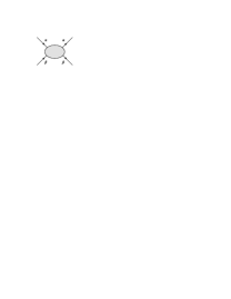
Figure 1: Four-fermion vertex function relevant to the calculation of the $\beta$-function.

The mass dimensions of the field and coupling are $[\![\chi_{0}]\!]=(D-2)/2$ and $[\![g_{0}]\!]=4-D$. We work in dimensional regularization and define the renormalized coupling $g(\mu)$ through $g_{0}=\overline{\mu}^{4-D}Z_{g}(\mu)\,g(\mu)$, where $\overline{\mu}^{2}\equiv\mu^{2}\,e^{\gamma_{E}}/(4\pi)$. The scale $\mu$ acts as an ultraviolet regulator in momentum space. Our renormalization factors will be defined using the modified minimal subtraction ($\overline{\rm MS}$) scheme in $D=4-\varepsilon$ space-time dimensions.

VI.1 Calculation of the $\beta$-function

Standard field-theory arguments can be used to show that the $\beta$-function of our model is given by

$$\beta(g,D)=\frac{dg(\mu)}{d\ln\mu}=\beta(g)+(D-4)\,g\,,$$ (68)

where

$$\beta(g)=g^{2}\,\frac{dZ_{g}^{(1)}}{dg}$$ (69)

is independent of $D$. The quantity $Z_{g}^{(1)}$ denotes the coefficient of the $1/\varepsilon$ pole in the Laurent expansion of the renormalization factor near $\varepsilon=0$. Throughout, we denote $g\equiv g(\mu)$ unless otherwise noted.

The $\beta$-function is obtained from the four-fermion vertex function with ingoing and outgoing component indices $\alpha\neq\beta$, shown in Figure 1. For simplicity we set the external momenta to zero. The tree-level contribution to the vertex function is given by the elementary vertex shown in Figure 2. At one-loop order there is a single loop topology but three different contractions of indices, depicted in Figure 3, which yield a multiplicity factor of $(4-N)$. At two-loop order there are three loop topologies, whose multiplicities can be obtained by analyzing the various possible contractions. The relevant diagrams and their group-theory factors are depicted in Figure 4. The two-loop scalar integrals required for our calculation can be obtained from Caffo:1998du .

Figure 2: Tree-level contribution to the vertex function.

Figure 3: One-loop contributions to the vertex function. The three graphs give rise to the same loop topology, shown on the right. The group-theory factors of the individual diagrams are $-(N-2)$, 1, 1, where the minus sign of the first graph results from the closed fermion loop.

Adding up the results for the various diagrams we obtain the bare vertex function. We then multiply this result by $Z_{\chi}^{2}$ to account for wave-function renormalization, and substitute $m_{0}^{2}=Z_{m^{2}}\,m^{2}$ and $g_{0}=\mu^{4-D}Z_{g}\,g$ to implement mass and coupling-constant renormalization. The renormalization factors $Z_{\chi}$ and $Z_{m^{2}}$ are determined from the calculation of the fermion self-energy in the next subsection. By requiring that the renormalized vertex function be finite, we extract

$$Z_{g}=1+\frac{4-N}{\varepsilon}\,g+\left[\frac{(4-N)^{2}}{\varepsilon^{2}}+\frac{3(3N-7)}{4\varepsilon}\right]g^{2}+O(g^{3})\,.$$ (70)

From eq. (69) we then obtain for the $\beta$-function

$$\beta(g)=(4-N)\,g^{2}+\frac{3(3N-7)}{2}\,g^{3}+O(g^{4})\,.$$ (71)

Figure 4: Two-loop topologies for the vertex function. Each topology receives contributions from several diagrams. The combined group-theory factors are listed below each graph.

The $D$-dimensional $\beta$-function in (68) has a non-trivial fixed point at positive coupling given by the solution to the equation $\beta(g_{*})/g_{*}=4-D=\varepsilon$. At second order in the $\varepsilon$-expansion, we find

$$g_{*}=\frac{\varepsilon}{4-N}+\frac{3(7-3N)}{2(4-N)^{3}}\,\varepsilon^{2}+O(\varepsilon^{3})\,.$$ (72)

VI.2 Calculation of the self-energy

Next we need the anomalous dimension of the fermion mass and field. They follow from a two-loop calculation of the self-energy $\Sigma(p^{2},m_{0}^{2})$ in the vicinity of the mass shell ($p^{2}=m^{2}$). Here $m_{0}$ and $m$ are the bare and renormalized mass parameters, respectively. The relevant relations are

$$m^{2}=m_{0}^{2}+\Sigma(m^{2},m_{0}^{2})\,,\qquad Z_{\chi}^{-1}=1-\Sigma^{\prime}(m^{2},m_{0}^{2})\,,$$ (73)

where the prime denotes a derivative with respect to the first argument, $p^{2}$. Inserting here $m_{0}^{2}=Z_{m^{2}}m^{2}$, one finds for the renormalization factors

$$Z_{m^{2}}=1-\frac{\Sigma(m^{2},Z_{m^{2}}m^{2})}{m^{2}}\,,\qquad Z_{\chi}^{-1}=1-\Sigma^{\prime}(m^{2},Z_{m^{2}}m^{2})\,.$$ (74)

At one-loop order there is a single tadpole graph to evaluate, while at two-loop order we have a double tadpole diagram and the sunrise diagram, see Figure 5. After accounting for coupling-constant renormalization using eq. (70), we obtain

$$Z_{m^{2}} = 1+\frac{1-N}{\varepsilon}\,g+(1-N)\left(\frac{5-2N}{2\varepsilon^{2}}-\frac{5}{8\varepsilon}\right)g^{2}+O(g^{3})\,,$$

$$Z_{\chi} = 1-\frac{1-N}{8\varepsilon}\,g^{2}+O(g^{3})\,.$$ (75)

The anomalous dimensions of the mass and field are given by

$$\gamma_{m^{2}}=-g\,\frac{dZ_{m^{2}}^{(1)}}{dg}\,,\qquad\gamma_{\chi}=-\frac{g}{2}\,\frac{dZ_{\chi}^{(1)}}{dg}\,,$$ (76)

where in the second relation we take into account that $\chi_{0}=\sqrt{Z_{\chi}}\,\chi$. We find

$$\gamma_{m^{2}}=2\gamma_{m} = (N-1)\,g\,\bigg{(}1-\frac{5}{4}\,g\bigg{)}+O(g^{3})\,,$$

$$\gamma_{\chi} = \frac{(1-N)}{8}\,g^{2}+O(g^{3})\,.$$ (77)

The anomalous dimension of the field starts at two-loop order. Instead of the anomalous dimension of $m^{2}$ one could compute the anomalous dimension of the fermion bilinear $\overline{\chi}\chi$, which is given by $\gamma_{\overline{\chi}\chi}=-\gamma_{m^{2}}$.

Figure 5: One- and two-loop diagrams contributing to the fermion self-energy.

Evaluating our expressions at the fixed-point value of the coupling yields

$$\gamma_{m} = \frac{(N-1)}{2(4-N)}\,\varepsilon\left[1+\frac{22-13N}{4(4-N)^{2}}\,\varepsilon\right]+O(\varepsilon^{3})\,,$$

$$\gamma_{\chi} = \frac{(1-N)}{8(4-N)^{2}}\,\varepsilon^{2}+O(\varepsilon^{3})\,.$$ (78)

As a crosscheck of our results, we note that the two-loop expressions for the $\beta$-function and anomalous dimensions obtained in eqs. (71) and (VI.2) go over to the corresponding results of $O(M)$ scalar field theory (see e.g. Zinn ) if we identify $M=-2N$. Likewise, the fixed-point of the fermionic $\beta$-function in eq. (72) is related to the Wilson-Fisher fixed point WilsonFisher by the same replacement rule. In some sense, our symplectic fermion theory may thus be considered as an analytic continuation of scalar $O(M)$ field theory to negative $M$. However, as emphasized in section IV, this simple correspondence is not expected to hold for all physical quantities.

VI.3 Renormalization of the composite bilinear $n_{\tau}$

The diagrams contributing to the renormalization of the composite operator $n_{\tau}=\overline{\chi}\,\tau\,\chi$ defined in eq. (65) can be obtained by inserting this operator into the one- and two-loop graphs for the fermion self-energy shown in Figure 5. In the evaluation of these graphs it is important to use that the matrix $\tau$ is traceless. Writing the bare current as $(n_{\tau})_{0}=Z_{n}n_{\tau}$, we obtain

$$Z_{n}=1-\frac{g}{\varepsilon}+\left(-\frac{3-N}{2\varepsilon^{2}}+\frac{5-N}{8\varepsilon}\right)g^{2}+O(g^{3})\,.$$ (79)

The anomalous dimension of the current is thus

$$\gamma_{n}=g-\frac{5-N}{4}\,g^{2}+O(g^{3})\,.$$ (80)

At the fixed point, this yields

$$\gamma_{n}=\frac{\varepsilon}{4-N}+\frac{(2-N)(11+N)}{4(4-N)^{3}}\,\varepsilon^{2}+O(\varepsilon^{3})\,.$$ (81)

This result will become important for the discussion in the following section.

VII Possible applications

In this section, we speculate on possible applications of the above results. The most interesting context is quantum criticality in $d=2$ spacial dimensions (i.e., $D=3$). In the broadest terms, since the particles have spin ${1\over 2}$, our model can describe a quantum critical theory of spinons.

Whereas the Mermin-Wagner theorem rules out continuous phase transitions at finite temperature in $d=2$, zero temperature quantum phase transitions continue to be of great interest. The best studied example is the quantum phase transition in $2d$ Heisenberg magnets, which is in the universality class of the $O(3)$ Wilson-Fisher fixed point Halperin ; Ye . One feature of our model is that it can describe quantum critical points wherein the magnetic order parameter ${\vec{n}}$ is a composite operator in terms of the more fundamental fermion fields. This could in principle have applications to quantum phase transitions in the anti-ferromagnetic phase of Hubbard-like models, where the magnetic order parameter is a bilinear in the electron fields. As stated in the introduction, if such electrons were described by the Dirac theory, the four-fermion interactions are irrelevant and do not generally lead to a low-energy interacting fixed point. That this is different in the case of symplectic fermions was the primary motivation for our work.

Let us first review the definitions of the exponents for the usual Wilson-Fisher fixed point. The order parameter is an $M$-component real vector ${\vec{n}}$ with action

$$S_{\rm WF}=\int d^{D}x\left[\partial{\vec{n}}\cdot\partial{\vec{n}}+m^{2}\,{\vec{n}}\cdot{\vec{n}}+\lambda\,({\vec{n}}\cdot{\vec{n}})^{2}\right].$$ (82)

Some of the exponents are defined with respect to perturbations away from the critical point. Namely, consider

$$S=S_{*}+\int d^{D}x\left(t\,{\cal O}_{\varepsilon}+\vec{B}\cdot{\vec{n}}\right),$$ (83)

where $S_{*}$ is the critical theory, ${\cal O}_{\varepsilon}$ is the “energy operator”, and $\vec{B}$ a magnetic field. For applications to classical statistical mechanics in $3D$ one identifies ${\cal O}_{\varepsilon}={\vec{n}}\cdot{\vec{n}}$ and $t=T-T_{c}$, so that $t\propto m^{2}$. The usual definition of the correlation-length exponent $\nu_{\epsilon}$ via $\xi\sim t^{-\nu_{\varepsilon}}$ then leads to

$$\nu_{\varepsilon}={1\over[\![t]\!]}={1\over D-[\![{\cal O}_{\varepsilon}]\!]}\,.$$ (84)

The second fundamental exponent is related to the scaling dimension of ${\vec{n}}$. It is conventional to parameterize this with $\eta$ in the form

$$[\![{\vec{n}}]\!]=\frac{D-2}{2}+\frac{\eta}{2}\,,$$ (85)

so that the two-point function at the critical point scales as

$$\langle{\vec{n}}(x)\cdot{\vec{n}}(0)\rangle\sim{1\over|x|^{D-2+\eta}}\,.$$ (86)

The convention for the leading contribution to $[\![{\vec{n}}]\!]$ comes from the action (82), which implies that classically ${\vec{n}}$ has dimension $(D-2)/2$. The parameter $\eta$ is then given as $\eta=2\gamma_{\vec{n}}$, where $\gamma_{\vec{n}}$ is the quantum anomalous correction to the scaling dimension of ${\vec{n}}$.

The third exponent characterize the one-point function of ${\vec{n}}$ via

$$\langle{\vec{n}}\rangle\sim t^{\beta}~{}\sim B^{1/\delta},$$ (87)

which leads to

$$\beta=\frac{[\![{\vec{n}}]\!]}{[\![t]\!]}=\frac{\nu_{\varepsilon}}{2}\,(D-2+\eta)\,.$$ (88)

Treating $\vec{B}$ as a coupling gives $[\![B]\!]+[\![{\vec{n}}]\!]=D$, from which it follows that

$$\delta=\frac{[\![B]\!]}{[\![{\vec{n}}]\!]}=\frac{D+2-\eta}{D-2+\eta}\,.$$ (89)

For the remainder of this section we consider the special case where $N=2$. In discussions of deconfined quantum criticality Senthil , for the case of $O(3)$ symmetry, the 3-vector ${\vec{n}}$ is represented as a bilinear in “spinon fields” $\chi$, i.e. ${\vec{n}}=\chi^{\dagger}\vec{\sigma}\,\chi$, where here $\chi$ is an $N=2$ component complex field and $\vec{\sigma}$ are the Pauli matrices. Note that $\vec{n}$ is an example of an operator $n_{\tau}$ defined in (65). For $N=2$, the above representation of ${\vec{n}}$ is consistent irrespective of whether $\chi$ is a boson or fermion, so we will treat both cases in parallel. If ${\vec{n}}$ is a rotational 3-vector, then $\chi$ is a spin-${1\over 2}$ doublet. This identification of spin is different than in section III, and is instead based on the $SU(2)$ sub-algebra generated by $\{1\otimes A,\sigma_{z}\otimes t_{z}\}$, where $t_{z}$ is traceless and symmetric (see section III for notations).

Simple considerations based on the renormalization group point to a possibly special role played by the $N=2$ fermion theory. Suppose a model formulated in terms of an $O(3)$ ${\vec{n}}$ field is asymptotically free in the ultraviolet region. Then the coefficient of the free energy $c_{D}$ described in section IV equals $3$ for any $D$. On the other hand, free $\chi$ fields give $c_{3}=3N/2$ by formula (44) in $3D$. which is the same as for the $O(3)$ ${\vec{n}}$ theory when $N=2$. Therefore, the free energies match up properly in the ultraviolet for an $O(3)$ ${\vec{n}}$ field and an $N=2$ symplectic fermion.

The model proposed in Senthil is based on the $CP^{1}$ representation of the non-linear $O(3)$ sigma model, which involves an auxiliary $U(1)$ gauge field. The $CP^{1}$ model is then modified by relaxing the non-linear constraint ${\vec{n}}\cdot{\vec{n}}=\chi^{\dagger}\chi=1$ and making the gauge field dynamical by adding a Maxwell term, effectively turning the model into an abelian Higgs model. One appealing feature of this model is that because of the equivalence of $CP^{1}$ and $O(3)$ non-linear sigma models (at least classically), without the Maxwell term one has an explicit map between the non-linear ${\vec{n}}$ field and $\chi$-field actions. Though this model is a natural candidate for a deconfined quantum critical point, unfortunately the fixed point is difficult to study perturbatively, so it has not been possible to accurately compare exponents with the simulations reported in Motrunich ; Sandvik .

Let us broaden the notion of deconfined quantum criticality to simply refer to a quantum critical point for an $O(3)$ vector order-parameter ${\vec{n}}$, where ${\vec{n}}$ is composite in terms of spinon fields $\chi$. The fields $\chi$ are interpreted as the fundamental underlying degrees of freedom, and the critical theory $S_{*}$ in eq. (83) is the critical theory for $\chi$. The critical exponents $\nu$, $\eta$, $\beta$, and $\delta$ defined above are then related to scaling dimensions of composite operators in the $S_{*}$ theory.

The anomalous dimension of ${\vec{n}}$ in the epsilon expansion follows from the results in section VI and will be denoted $\gamma_{\vec{n}}$ in what follows. Let us first consider the case where $\chi$ is a bosonic field. As explained above, the exponents for bosonic verses fermionic theories are simply related by $N\to-N$. Specializing eq. (81) to $N=-2$ in $3D$ ($\varepsilon=1$) one finds $\gamma_{\vec{n}}\approx 0.21$ for bosonic $\chi$. This is quite large compared to the analogous result $\gamma_{\vec{n}}\approx 0.02$ for the $O(3)$ Wilson-Fisher fixed point. (The latter is well-known; as explained in section V, it corresponds to $\gamma_{\chi}$ at $N=-3/2$.) For $\chi$ a fermion, interestingly the $O(\varepsilon^{2})$ correction to the leading one-loop result vanishes for $N=2$, so that $\gamma_{\vec{n}}=1/2$. We can give an alternative estimate of $\gamma_{\vec{n}}$ by simply substituting $g_{*}=11/16$ from eq. (72) into (80) without expanding in $\varepsilon$. This gives $\gamma_{\vec{n}}\approx 0.33$ for fermionic $\chi$. For both the bosonic and fermionic cases, the largeness of $\gamma_{\vec{n}}$ compared with the usual $O(3)$ fixed point is due to the compositeness of ${\vec{n}}$. If we naturally identify ${\cal O}_{\varepsilon}$ with ${\overline{\chi}}\chi$, then the correlation-length exponent $\nu_{\varepsilon}$ is given by eqs. (52) and (VI.2) evaluated with $N=\pm 2$. This leads to

$$\nu_{\varepsilon}\approx 0.75~{}~{}({\rm{bosonic}})\,,\qquad\nu_{\varepsilon}\approx 0.42~{}~{}({\rm fermionic})\,.$$ (90)

There are at least two difficulties encountered if we attempt to compare with existing numerical simulations, such as those in Motrunich ; Sandvik . The main one is that the simulations are performed with an action for the ${\vec{n}}$ field or for local lattice spin variables $\vec{S}_{i}$ with a Heisenberg-like hamiltonian, rather than with fundamental spinon degrees of freedom $\chi$, and we do not have a direct map between the two descriptions. In particular, in a theory with fundamental $\chi$ fields and the compositeness relation ${\vec{n}}=\chi^{\dagger}\vec{\sigma}\,\chi$, since $\chi$ has classical dimension $(D-2)/2$, one has

$$[\![{\vec{n}}]\!]=D-2+\gamma_{\vec{n}}\,.$$ (91)

Comparing with eq. (85) one finds $\eta=D-2+2\gamma_{\vec{n}}$ rather than the usual relation $\eta=2\gamma_{\vec{n}}$. In other words, $\eta$ now contains a purely classical contribution of $D-2$, and this was used to argue that the $\eta$ exponent was large in Senthil . On the other hand, simulations based on ${\vec{n}}$-field actions effectively force the classical contribution to $[\![{\vec{n}}]\!]$ to be $(D-2)/2$ as in the Wilson-Fisher theory, suggesting that simulations measure $\eta=2\gamma_{\vec{n}}$. In the fermionic theory, support for this idea comes from the fact that the two lowest orders of the $\varepsilon$ expansion give $\gamma_{\vec{n}}=1/2$ in $D=3$.

The other difficulty is that, unlike for temperature phase transitions where $t=T-T_{c}$, in the context of zero temperature quantum critical points it is not obvious what plays the role of the parameter $t$, or equivalently, the energy operator ${\cal O}_{\varepsilon}$ that determines the correlation-length exponent. In this context, $t$ is a parameter in the hamiltonian that is tuned to the critical point. The most natural choice is ${\cal O}_{\varepsilon}={\overline{\chi}}\chi$ which implies $t=m^{2}$ and leads to eq. (90). However, another possibility could be $t=m$, which would lead to twice the values in eq. (90), corresponding to $\nu_{\varepsilon}=1/(1+{\gamma_{m}})$.

The above difficulties prevent us from establishing a definite connection with the simulations in Motrunich ; Sandvik . In fact, the exponents for deconfined quantum criticality are currently controversial, since the two above works disagree strongly on the value of the exponent $\eta$. However, we point out that if one identifies $\eta=2\gamma_{\vec{n}}$, then our computed exponents are not inconsistent with some of the exponents in Motrunich ; Sandvik , although the comparison is not conclusive. More specifically, the work Motrunich reports $\eta\approx 0.6$–0.7 and $\nu=0.8$–1.0. On the other hand, for a different model Sandvik , it was found that $\eta=0.26\pm 0.03$ and $\nu=0.78\pm 0.03$. Both simulations are consistent with $\nu_{\varepsilon}$ in eq. (90) for a bosonic spinon and $t=m^{2}$. However, they are also consistent with a fermionic spinon with $t=m$. Our formulas give $\eta\approx 0.67$ and $\eta\approx 0.42$ for fermions and bosons, respectively.

VIII Conclusions

To summarize, we proposed that spin-${1\over 2}$ particles can be described by a symplectic fermion quantum field theory as an alternative to the Dirac theory if one demands only rotational invariance rather than the full Lorentz invariance. The resulting lagrangian has a form resembling that of a scalar field but with the “wrong” statistics. A hidden $Sp(2N)$ symmetry allows identification of spin via an $SO(3)$ subgroup for any $N$, so that the statistics of the field is consistent with the spin-statistics connection for spin-${1\over 2}$ particles. The hamiltonian is pseudo-hermitian, and this is sufficient to guarantee a unitary time evolution. The usual spin-statistics theorem for this kind of field theory is circumvented, because the proof of the latter does not allow for a pseudo-hermitian hamiltonian.

We have analyzed the renormalization-group properties and critical exponents of the symplectic fermion model up to two-loop order. The anomalous dimensions and $\beta$-function of the $Sp(2N)$ model are related to those of the $O(M)$ Wilson-Fisher model by setting $M=-2N$. This correspondence between $O(M)$ and $Sp(2N)$ models does not hold for all physical properties however. In addition to the usual exponents, we have also computed exponents for fields that are bilinear in the fundamental spinon fields.

The potentially most interesting possible applications of our theory are to quantum critical spinons in $d=2$ spacial dimensions. We have computed the critical exponents for “magnetic” order parameters that are quadratic in the spinon fields, as in models of deconfined quantum criticality. Comparison with existing numerical simulations is to some extent favorable, but not yet conclusive.

Acknowledgments

One of us (A.L.) would like to thank C. Henley, A. Ludwig, F. Nogeira, N. Read, S. Sachdev, A. Sandvik, T. Senthil, and J. Sethna for useful discussions. This research was supported in part by the National Science Foundation under Grant PHY-0355005.

References

- (1) K. S. Novoselov, A. K. Geim, S. V. Morozov, D. Jiang, M. I. Katsnelson, I.V Grigorieva, S. V. Dubonos and A. A. Firsov, Nature 438 (2005) 197 [cond-mat/0509330].
- (2) Y. Zhang, Y.-W. Tan, H. L. Stormer and P. Kim, Nature 438 (2005) 201.
- (3) W. Pauli, Rev. Mod. Phys. 15 (1943) 175.
- (4) A. Mostafazadeh, J. Math. Phys. 43 (2002) 205.
-
(5)
C. M. Bender and S. Boettcher,
Phys. Rev. Lett. 80 (1998) 5243
[physics/9712001];
C. M. Bender, F. Cooper, P. N. Meisinger and V. M. Savage, Phys. Lett. A259 (1999) 224 [quant-ph/9907008];
C. M. Bender, D. C. Brody and H. F. Jones, Phys. Rev. Lett. 89 (2002) 270401 [quant-ph/0208076]. - (6) C. M. Bender, Making sense of non-Hermitian Hamiltonians, preprint hep-th/0703096.
-
(7)
K. G. Wilson and M. E. Fisher,
Phys. Rev. Lett. 28 (1972) 240;
K. G. Wilson and J. Kogut, Phys. Rep. 12 (1974) 75. - (8) A. LeClair, Quantum critical spin liquids and conformal field theory in dimensions, preprint cond-mat/0610639.
- (9) T. Senthil, L. Balents, S. Sachdev, A. Vishwanath and M. P. A. Fisher, Phys. Rev. B70 (2004) 144407 [cond-mat/0312617].
- (10) A. LeClair, 3D Ising and other models from symplectic fermions, preprint cond-mat/0610817.
- (11) S. Weinberg, Quantum Theory of Fields I, Cambridge University Press, 1995.
- (12) H. Georgi, Lie Algebras in Particle Physics, Frontiers in Physics, vol. 54, 1982.
- (13) A. A. Belavin, A. M. Polyakov and A. B. Zamolodchikov, Nucl. Phys. B241 (1984) 333.
- (14) H. G. Kausch, Curiosities at , preprint hep-th/9510149.
- (15) D. Friedan, E. Martinec and S. Shenker, Nucl. Phys. B271 (1986) 93.
- (16) H. Saleur, Nucl. Phys. B382 (1992) 486 [hep-th/9111007].
- (17) M. Caffo, H. Czyz, S. Laporta and E. Remiddi, Nuovo Cim. A 111, 365 (1998) [hep-th/9805118].
- (18) J. Zinn-Justin, Quantum Field Theory and Critical Phenomena, 2nd ed., Oxford Univ. Press, 1993.
- (19) S. Chakravarty, B. I. Halperin and D. R. Nelson, Phys. Rev. B39 (1989) 2344.
- (20) A. V. Chubukov, S. Sachdev and J. Ye, Phys. Rev. B49 (1994) 11919 [cond-mat/9304046].
- (21) O. I. Motrunich and A. Vishwanath, Phys. Rev. B70 (2004) 075104 [cond-mat/0311222].
- (22) A. W. Sandvik, preprint cond-mat/0611343.