Relativistic Multiple Scattering Theory and the Relativistic Impulse Approximation

Abstract

It is shown that a relativistic multiple scattering theory for hadron-nucleus scattering can be consistently formulated in four-dimensions in the context of meson exchange. We give a multiple scattering series for the optical potential and discuss the differences between the relativistic and non-relativistic versions. We develop the relativistic multiple scattering series by separating out the one boson exchange term from the rest of the Feynman series. However this particular separation is not absolutely necessary and we discuss how to include other terms. We then show how to make a three-dimensional reduction for hadron-nucleus scattering calculations and we find that the relative energy prescription used in the elastic scattering equation should be consistent with the one used in the free two-body $t$-matrix involved in the optical potential. We also discuss what assumptions are involved in making a Dirac Relativistic Impulse Approximation (RIA).

1 Introduction

The Relativistic Impulse Approximation (RIA) is one of the most successful tools in describing hadron-nucleus scattering observables. At the beginning it was prompted by the success of Dirac phenomenology [1] in describing proton-nucleus scattering where a parameterized optical potential was used in a Dirac equation. Soon after this, guided by the non-relativistic $t\rho$ approximation of the optical potential, a relativistic generalization (RIA) was made [2]. Over the years other authors [3, 4] have also successfully used the RIA with various prescriptions for the $t$-matrix and the target density. In the case of meson-nucleus scattering, the RIA optical potential was successfully used in the Kemmer-Duffin-Patiau equation [5]. Recently, a Dirac-RIA was used in analyzing neutron densities [6] and nuclear densities arising from chiral models [7]. which shows that the RIA is also useful in the studies of the bulk properties of nuclear matter.

The RIA is a very useful tool in medium energy nuclear physics. It is based upon the existence of a multiple scattering theory which obviously must have some resemblance to non-relativistic multiple scattering theory. In the non-relativistic theory, there is no ambiguity in what equation is to be used as the scattering equation. There is only one equation available, namely the Schrodinger equation. For the NN amplitudes, there are several possible choices. Some are pure phenomenological fits and some are calculated from potential models.

In the relativistic case, even the use of Dirac equation in nucleon-nucleus scattering is questionable. At best, the use of the Dirac equation can be a good approximation. When the Dirac equation is used in describing the passage of the projectile nucleon through the nucleus, the tacit assumption is that the nucleus is infinitely heavy, but in reality it is not. There are also ambiguities in choosing the NN amplitude to be used in the RIA optical potential, since there are in principle infinitely many relativistic two-body quasi-potential equations that can be used in producing NN amplitudes. In order to address these issues, it is important to develop a relativistic multiple scattering theory (RMST). As far as we are aware, there has been only one attempt to develop an RMST which was done by Maung and Gross [8, 9]. In their approach they start from the sum of all meson exchange diagrams between the projectile and target nucleus. By considering the cancellation between the box and crossed-box diagrams, they concluded that the projectile-target propagator should be a three-dimensional propagator with the target on mass-shell when the target is in the ground state. In order to avoid spurious singularities, Maung and Gross chose the propagator with the projectile nucleon on mass-shell when the target is in the excited state. They developed an RMST and argued that the NN amplitude that should be used in the RIA optical potential should be calculated from a covariant 3-dimensional equation with one particle on-mass-shell.

We revisit the formulation of an RMST using a meson exchange model. Since the cancellation of the box and crossed-box diagrams does not work satisfactorily when spin and isospin are included, we develop an RMST which is independent of this cancellation. The paper is organized as follows. We briefly review the non-relativistic multiple scattering formalism of Watson [10]. We then develop an RMST for the optical potential from a meson exchange model in four-dimensions. Also we discuss what is involved in making the Relativistic Impulse Approximation. Finally we discuss the validity of using the Dirac equation for proton-nucleus scattering and examine the alternatives. This paper makes reference only to pion exchange, but in principle any number of different boson exchanges, such as $\sigma$, $\rho$, $\omega$ etc. could be included. One only has to replace the pion exchange with these other bosons. In this paper we emphasize the multiple scattering formalism and not the calculation of nucleon-nucleon amplitudes, and hence we do not make any specification of meson-nucleon couplings or form factors to be used. In the literature numerous authors over the years have used different relativistic equations and meson-nucleon couplings and various types of form factors have been employed in nucleon-nucleon phenomenology.

2 Review of non-relativistic theory

This section contains a review of non-relativistic theory following references [4, 9, 11, 12, 13, 14], which provide an introduction to the topics of non-relativistic [11, 12, 13] and relativistic [4, 9, 11, 14] multiple scattering theory. This review is included so that the reader can more easily understand the new relativistic multiple scattering theory introduced later in the paper. The full $pA$ hamiltonian is given by

$$H=H_{0}+V=h_{0}+H_{A}+V$$ (1)

where $h_{0}$ is the kinetic energy operator of the projectile and $H_{A}$ is the full $A$-body hamiltonian of the target. $H_{A}$ contains all the target nuclear structure information with

$$H_{A}=\sum\limits_{i=1}^{A}h_{i}+\sum\limits_{i<j}^{A}v_{ij}$$ (2)

This target Hamiltonian is just the sum of the target nucleon kinetic energies plus the sum of their pair interactions [11]. The residual interaction $V$ is given by the sum of the interactions between the projectile and target particles,

$$V=\sum\limits_{i=1}^{A}v_{0i}$$ (3)

where $v_{0i}$ denotes the interaction between the projectile, labeled particle “0” and the target nucleon labeled with index “$i$”. We also write the $T$-matrix,

$$T \equiv \sum\limits_{i=1}^{A}T_{0i}$$ (4)

This and equation (3) are shown using diagrams defined in Figure 1 and defined in this way, the diagrams themselves can then be easily iterated, as shown later.

Figure 1: Diagrams of the definitions $V\equiv\sum\limits_{i=1}^{A}v_{0i}$ (top) and $T\equiv\sum\limits_{i=1}^{A}T_{0i}$ (bottom) for a target containing 3 particles.

The eigenstates (i.e. nuclear bound states) of the nuclear target Hamiltonian $H_{A}$ satisfy

$$H_{A}|\phi_{n}^{A}\rangle=E_{n}|\phi_{n}^{A}\rangle$$ (5)

From the beginning the A-body problem is separated from the rest and we assume that there is some means of obtaining the solution of this A-body bound state problem. The projectile scattering eigenstates satisfy

$$h_{0}|{\bf k}\rangle=E_{k}|{\bf k}\rangle$$ (6)

The eigenstates of the full unperturbed $pA$ Hamiltonian $H_{0}=h_{0}+H_{A}$ satisfy

$$H_{0}|\Phi\rangle=E|\Phi\rangle$$ (7)

where the energy $E$ is total kinetic energie of the projectile and target plus the eigenenergies of the target. In the lab frame the target kinetic energy is zero. The initial and final states are

$$|\Phi_{i}\rangle=|\phi_{i}\rangle|{\bf k}_{i}\rangle\;,\hskip 42.67912pt|\Phi_{f}\rangle=|\phi_{f}\rangle|{\bf k}_{f}\rangle$$ (8)

The transition amplitude between different intial and final states of the same energy is

$$T_{fi}\equiv\langle\Phi_{f}|T|\Phi_{i}\rangle$$ (9)

with the $T$ matrix operator given by the Lippman-Schwinger equation (LSE),

$$T=V+VG_{0}T$$ (10)

where the free propagator of the $pA$ system is

$$G_{0}=\frac{1}{E-H_{0}+i\eta}=\frac{1}{E-h_{0}-H_{A}+i\eta}$$ (11)

The diagrammatic representation of the LSE is shown in Figure 2. Note that there are three energies involved in the evaluation of $\langle{\bf k}_{f}|T(E)|{\bf k}_{i}\rangle$, where the energy $E$ in $T(E)$ is the energy appearing in $G_{0}$ above and in equation (7). There is also the initial energy of the projectile $E_{i}$ and the final energy $E_{f}$ of the scattered projectile and any emitted particles. If the three energies are all different the process is described as completely off-energy-shell [12] and we have the completely off-energy-shell $T$-matrix $\langle{\bf k}_{f}|T(E)|{\bf k}_{i}\rangle$ [12]. We can also define two half off-energy-shell $T$-matrices as $\langle{\bf k}_{f}|T(E_{i})|{\bf k}_{i}\rangle$ or $\langle{\bf k}_{f}|T(E_{f})|{\bf k}_{i}\rangle$ when $E=E_{i}$ or $E=E_{f}$. These three amplitudes become equal in the completely on-energy-shell situation where $E=E_{i}=E_{f}$ [12].

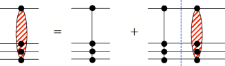
Figure 2: Diagram of the Lippman-Schwinger equation, $T=V+VG_{0}T$, for nucleon-nucleus scattering. The propagator $G_{0}=\frac{1}{E-h_{0}-H_{A}+i\eta}$ is shown by the vertical dashed line, which goes through all of the nucleons in the target because the propagator contains the full nuclear hamiltonian $H_{A}$.

2.1 First order multiple scattering

Substituting (3) into (10) gives what we call the Lippman-Schwinger expansion,

$$T=\sum\limits_{i=1}^{A}v_{0i}+\sum\limits_{i=1}^{A}v_{0i}G_{0}T$$ (12)

with the $i^{\rm th}$ term

$$T_{0i} \equiv v_{0i}+v_{0i}G_{0}T=v_{0i}+v_{0i}G_{0}\sum\limits_{j}T_{0j}$$ (13)

which, upon iteration gives [11]

$$T_{0i}\equiv v_{0i}+v_{0i}G_{0}\sum\limits_{j}v_{0j}+\cdots$$ (14)

Suppose the target is a nucleus with three nucleons. Then this expression is

$$T_{0i} \equiv v_{0i}+v_{0i}G_{0}(v_{01}+v_{02}+v_{03})+\cdots$$ (15)

where the first term represents a single interaction between the projectile and the $i$-th target nucleon. The collection of second terms represent a double interaction between the projectile and the $i$-th target nucleon. This consists of a single interaction between the projectile and the $i$-th target nucleon, followed by propagation represented by $G_{0}$ and then another single interactions between the projectile and each of the target nucleons. Figures 3 and 4 show the series for a proton scattering from a nucleus with three nucleons. One can see that the diagram definitions in Figure 1 allows for the diagrams themselves to be iterated as in Figures 3 and 4.

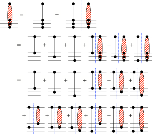
Figure 3: Diagram of the Lippman-Schwinger equation and its expansion,
$T=V+VG_{0}T=\sum\limits_{i=1}^{A}v_{0i}+\sum\limits_{i=1}^{A}v_{0i}G_{0}T=\sum\limits_{i=1}^{A}v_{0i}+\sum\limits_{i=1}^{A}v_{0i}G_{0}\sum\limits_{j}T_{0j}$

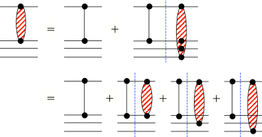
Figure 4: Diagram of the $i^{\rm th}$ term of the Lippman-Schwinger equation and its expansion, $T_{0i}=v_{0i}+v_{0i}G_{0}T=v_{0i}+v_{0i}G_{0}\sum\limits_{j}T_{0j}$

Each higher order term in (14) contains terms where the interaction occurs multiple times on the same target nucleon. These can be separated off by writing

$$T_{0i} = v_{0i}+v_{0i}G_{0}v_{0i}+v_{0i}G_{0}v_{0i}G_{0}v_{0i}\cdots+v_{0i}G_{0}\sum\limits_{j\neq i}v_{0j}+\cdots$$ (16)

$$= t_{0i}+v_{0i}G_{0}\sum\limits_{j\neq i}v_{0j}+\cdots$$ (17)

with (see Figure 5)

$$t_{0i} \equiv v_{0i}+v_{0i}G_{0}t_{0i}=v_{0i}+v_{0i}G_{0}v_{0i}+v_{0i}G_{0}v_{0i}G_{0}v_{0i}+\cdots$$ (18)

Figure 5: Diagram of the single scattering term, $t_{0i}\equiv v_{0i}+v_{0i}G_{0}t_{0i}=v_{0i}+v_{0i}G_{0}v_{0i}+v_{0i}G_{0}v_{0i}G_{0}v_{0i}+\cdots$

Write equation (13) as

$$T_{0i} \equiv v_{0i}+v_{0i}G_{0}T=v_{0i}+v_{0i}G_{0}\sum\limits_{j}T_{0j}$$ (19)

$$= v_{0i}+v_{0i}G_{0}T_{0i}+v_{0i}G_{0}\sum\limits_{j\neq i}T_{0j}$$ (20)

Rearrange as

$$(1-v_{0i}G_{0})T_{0i} = v_{0i}+v_{0i}G_{0}\sum\limits_{j\neq i}T_{0j}$$ (21)

giving

$$T_{0i} = (1-v_{0i}G_{0})^{-1}v_{0i}+(1-v_{0i}G_{0})^{-1}v_{0i}G_{0}\sum\limits_{j\neq i}T_{0j}$$ (22)

Using the binomial series $\frac{1}{1-x}=1+x+x^{2}+\cdots$ gives

$$(1-v_{0i}G_{0})^{-1}v_{0i} = v_{0i}+v_{0i}G_{0}v_{0i}+v_{0i}G_{0}v_{0i}G_{0}v_{0i}+\cdots=t_{0i}$$ (23)

to finally give the Watson multiple scattering series [10, 11, 12]

$$T_{0i} = t_{0i}+t_{0i}G_{0}\sum\limits_{j\neq i}T_{0j}$$ (24)

The advantage of this series is that it is an expression for the full $T$ matrix involving scattering amplitudes $t_{oi}$ rather than potentials $v_{oi}$, with each $t_{oi}$ containing an infinite number of the $v_{oi}$ terms.

2.2 Single scattering approximation (SSA)

The single scattering approximation is

$$T_{0i}\approx t_{0i}$$ (25)

so that (12) becomes

$$T\equiv\sum\limits_{i=1}^{A}T_{0i}\approx\sum\limits_{i=1}^{A}t_{0i}=t_{01}+t_{02}+t_{03}+\cdots$$ (26)

The single scattering approximation is shown in Figure 6, and “may be valid for weak scattering or for dilute systems. This works for electron scattering” [12]. Tandy [11] mentions that the SSA “makes a great deal of sense, since the projectile, once it comes close to a given target particle may multiply interact with that particle, but once it is ejected will, with a high degree of probability, “miss” all the other target particles.”

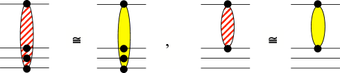
Figure 6: Diagram of the single scattering approximation $T\approx\sum\limits_{i=1}^{A}t_{0i}$ (left diagram) or the $i^{\rm th}$ term $T_{0i}\approx t_{0i}$ (right diagram).

2.3 Impulse approximation (IA)

Tandy explains the SSA as follows [11]. “The required amplitude described by $t_{0i}$ does not correspond to the solution of a (free) nucleon-nucleon scattering problem. Because of the presence of $H_{A}$ in the Green’s function operator $G_{0}$ of equation (18), the motion of nucleon $i$ is governed not only by its interaction $v_{0i}$ with the projectile, but also by its interaction with the other constituents of the target. A further approximation can be envisaged in which $H_{A}$ is assumed to simply set an energy scale so that the solution of equation (18) might be replaced by the solution of a free nucleon-nucleon scattering problem. With this interpretation of $t_{0i}$, equation (26) is referred to as the impulse approximation.” Thus there are two pieces to the single scattering IA The first piece consists of the SSA but with the replacement [12]

$$t_{0i}\approx t_{0i}^{\rm free}$$ (27)

and the second piece consists of using the free Green function

$$G_{0}\equiv\frac{1}{E-h_{0}-H_{A}}\;\;\approx\;\;G_{0}^{\rm free}\equiv\frac{1}{E-h_{0}-h_{i}}$$ (28)

This essentially means that the target nucleus is treated as though it is not bound.

2.4 Optical potential and Watson series

For elastic scattering it is useful to use an optical potential which reduces the orginal many-body elastic scattering problem to a one-body problem. All the complicated many-body problems are now included in the optical potential. Therefore for practical calculations approximations have to be made to determine the optical potential to be used in the scattering equation. We follow Feshbach [11, 15, 16] and define a ground state projector P and an operator Q which projects onto the complementary space of the excited target states including inelastic break-up states [11, 15, 16] so that

$$P+Q=1$$ (29)

where the projector of the target ground state is

$$P\equiv|\phi_{0}\rangle\langle\phi_{0}|$$ (30)

with $|\phi_{0}\rangle$ denoting the target nuclear ground state, giving

$$P|\phi_{\alpha}\rangle=|\phi_{0}\rangle\langle\phi_{0}|\phi_{\alpha}\rangle=|\phi_{0}\rangle\delta_{\alpha 0}=|\phi_{0}\rangle$$ (31)

Now for elastic scattering the initial and final states are the ground state [11], namely

$$|\phi_{i}\rangle_{\rm elastic}=|\phi_{f}\rangle_{\rm elastic}=|\phi_{0}\rangle$$ (32)

so that

$$T_{fi\;\rm elastic}\equiv\langle\Phi_{f}|T|\Phi_{i}\rangle_{\rm elastic}=\langle{\bf k}_{f}|\langle\phi_{f}|T|\phi_{i}\rangle|{\bf k}_{i}\rangle = \langle{\bf k}_{f}|\langle\phi_{0}|T|\phi_{0}\rangle|{\bf k}_{i}\rangle$$ (33)

$$= \langle\Phi_{f}|PTP|\Phi_{i}\rangle$$ (34)

Thus for elastic scattering

$$T_{\rm elastic}\equiv PTP$$ (35)

In analogy with the LSE (10), define the optical potential as [11]

$$PTP\equiv PUP+PUPG_{0}PTP$$ (36)

or

$$T \equiv U+UPG_{0}T$$ (37)

$$U = V+VG_{0}QU$$ (38)

This will help us obtain the microscopic content of the optical potential. Equations (37) and (38) are completely equivalent to the Lippman-Schwinger equation (10). This is easily seen by writing $U=(1-VG_{0}Q)^{-1}V$ and substitute into (37). Multiply the new (37) by $1-VG_{0}Q$ and (10) results. Because $P^{2}=P$ and $Q^{2}=Q$ and $P$, $Q$ both commute with $G_{0}$, then instead of (37) and (38) we can define $U$ differently and write

$$T \equiv U+UPG_{0}PT$$ (39)

$$U = V+VQG_{0}QU$$ (40)

These equations are also completely equivalent to the Lippman-Schwinger equation (10). We shall use the above two equations, instead of (37) and (38) from now on. Following definition (12) we now define

$$U\equiv\sum\limits_{i=1}^{A}U_{0i}$$ (41)

and similar to equation (13), we have

$$U_{0i} = v_{0i}+v_{0i}QG_{0}QU=v_{0i}+v_{0i}QG_{0}Q\sum\limits_{j}U_{0j}$$ (42)

Now define [10, 17] an operator $\tau_{i}$

$$\tau_{0i} \equiv v_{0i}+v_{0i}QG_{0}Q\tau_{0i}$$ (43)

which is analogous to (18). Therefore we get the Watson multiple scattering series for the optical potential [10, 11, 17]

$$U_{0i} = \tau_{0i}+\tau_{0i}QG_{0}Q\sum\limits_{j\neq i}^{A}U_{0j}$$ (44)

analogous to (24). Summing gives

$$U = \sum\limits_{i=1}^{A}\tau_{0i}+\sum\limits_{i=1}^{A}\tau_{0i}QG_{0}Q\sum\limits_{j\neq i}^{A}U_{0j}=\sum\limits_{i=1}^{A}\tau_{0i}+\sum\limits_{i=1}^{A}\tau_{0i}QG_{0}Q\sum\limits_{j\neq i}^{A}\tau_{0j}+\cdots$$ (45)

One may ask why we went to all this trouble to develop an optical theory. Why don’t we just calculate the ground state $T$-matrix element $\langle 0|T|0\rangle$? We could calculate matrix elements using either the Lippman-Schwinger expansion in equation (12) or the Watson series in equation (24). The trouble is that both equations involve $G_{0}$, which we have seen involves a sum over all excited states, which makes the LSE very difficult to solve. However with $T$ expressed in terms of $U$ in equation (39), we see that it contains the term $PG_{0}P$ which means that it only includes intermediate states with the target in the ground state. The single scattering approximation or the first order optical potential is obtained by keeping the first term only. The successive terms can be interpreted as the double scattering term, triple scattering terms etc. and hence the name multiple scattering. The first order Watson optical potential is [9]

$$U = \sum\limits_{i=1}^{A}\tau_{0i}$$ (46)

but $\tau$ is not the free two-body $t^{\rm free}$ matrix because of the presence of the many body propagator $QG_{0}Q$ in (43), where all intermediate states are in excited states. For practical calculations a free two-body $t$-matrix is more easily available. The free two-body $t$ matrix is defined

$$t^{\rm free}_{0i}\equiv v_{0i}+v_{0i}gt^{\rm free}_{0i}$$ (47)

where $g$ is the free two body propagator. The relation between $t^{\rm free}$ and the Watson operator $\tau$ is

$$\tau_{0i}=t^{\rm free}_{0i}+t^{\rm free}_{0i}(QG_{0}Q-g)\tau_{0i}$$ (48)

For high projectile energies one usually approximates $\tau$ by $t^{\rm free}$ (impulse approximation) and obtains the first order Watson impulse approximation optical potential

$$U^{1\rm st}_{\rm impulse} = \sum\limits_{i=1}^{A}t^{\rm free}_{0i}$$ (49)

The Watson optical potential in terms of the free two body $t$ matrix is usually written

$$U = \sum\limits_{i=1}^{A}t_{0i}^{\rm free}+\sum\limits_{i=1}^{A}t_{0i}^{\rm free}(QG_{0}Q-g)U_{0i}+\sum\limits_{i=1}^{A}\sum\limits_{j\neq i}^{A}t_{0i}^{\rm free}QG_{0}QU_{0j}$$ (50)

$$= \sum\limits_{i=1}^{A}t_{0i}^{\rm free}+\sum\limits_{i=1}^{A}t_{0i}^{\rm free}(QG_{0}Q-g)t^{\rm free}_{0i}+\sum\limits_{i=1}^{A}t_{0i}^{\rm free}QG_{0}Q\sum\limits_{j\neq i}^{A}t^{\rm free}_{0j}+\cdots$$ (51)

up to second order. Obviously the first term is the single scattering term, the second term is the single scattering propagator correction term and the third term is the double scattering term etc. The first term alone gives the single scattering or the first-order Impulse Approximation (IA) optical potential operator. It is important to note that it is not the same as approximating the Watson $\tau$ with free $t$-matrix at the single scattering level. As can be seen from the above equation there also is a propagator correction term at the single scattering level although it is second order in $t$. Actually the propagator correction term exists to all orders for each level of scattering, i.e. for single scattering, double scattering etc. The propagator correction term can be interpreted as the medium correction term since it corrects the use of free propagator instead of the propagator with the excited intermediate target state. For high projectile energies the differences between $\tau$ and $t^{\rm free}$ become negligible. The last term represents the multiple scattering. For non-relativistic calculations $t^{\rm free}$ can be obtained from (47) by using a choice of $v$ such as the Reid potential.

3 Relativistic multiple scattering

Now we discuss a formulation of an RMST in the context of meson exchange. That is, the interaction between the projectile and the A-body target nucleus will be mediated by meson exchange. We start from the fact that the $t$-matrix for the relativistic projectile-target scattering is given by the Bethe-Salpeter equation where the kernel is the sum of all two-body (projectile and the A-body target nucleus) irreducible diagrams. The derivation of a multiple scattering series from a field theoretical Lagrangian is a very difficult and open problem. We want to develop a multiple scattering theory from the meson exchange point of view and want to see what approximations are involved in the RIA. Therefore in all the diagrams, all self energy and vertex corrections are included as renormalized masses and vertices with form factors. The kernel of the equation is denoted by $V$ and diagrams up to the fourth order in the meson-nucleon coupling are shown in Figure 7.

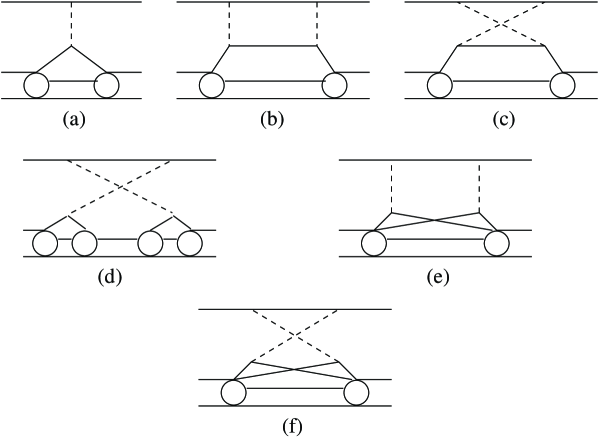
Figure 7: Diagrams in the kernel of the nucleon-nucleus Bethe-Salpeter equation up to the fourth order in the coupling. The projectile is represented by a single line and the target is represented by a double line.

The Bethe-Salpeter equation for the scattering is

$$T=V+VG_{0}T$$ (52)

where $G_{0}$ is the four-dimensional two-body propagator of the projectile-target system. The first term in $V$ shown in Figure 7a is the sum of one boson exchange interactions between the projectile and the target nucleons. We label these by $\sum\limits_{i}K_{0i}$. The second and the third diagrams shown in Figure 7b and 7c are the two meson exchange diagrams between the projectile and the $i^{\rm th}$ target nucleon and we will denote them by $\sum\limits_{i}K_{ii}^{(1)}$ and $\sum\limits_{i}K_{ii}^{(2)}$. In a similar manner we will denote third and higher order diagrams involving multi-meson exchange between the projectile and a single target nucleon by $\sum\limits_{i}K_{iii}^{(m)}$, $\sum\limits_{i}K_{iiii}^{(m)}$ etc. The box diagrams are labeled with $m=1$ and the cross box diagrams are labeled with $m=2$. Next we notice that there exist irreducible multi-meson exchange diagrams between the projectile and the target nucleus shown in Figures 7d, 7e and 7f. Since our aim is to write a multiple scattering theory similar to the non-relativistic theory, we need to classify the diagrams in some way so that the kernel $V$ can be indexed by the nucleon index. For example, we can label the diagram in Figure 7d by $\sum_{ij}L_{ij}$ and Figure 7e and 7f by $\sum_{i,j\neq i}M_{ij}^{(1)}$ and $\sum_{i,j\neq i}M_{ij}^{(2)}$ etc. Now it is obvious that every diagram can be written in the form $\sum\limits_{i}F_{i}$. From experience with the non-relativistic theory, we know that at a later point, we would like do the resummation of the Born series in terms of a free $t$-matrix and in the relativistic case, it might be a $t$-matrix calculated from some One Boson Exchange (OBE) model. Thus we can separate $K_{0i}$ from the rest of the terms in the kernel, as in

$$V=\sum\limits_{i=0}^{A}V_{0i}=\sum\limits_{i=0}^{A}(K_{0i}+\Lambda_{0i})$$ (53)

with

$$\Lambda_{0i}\equiv\sum\limits_{i}\sum\limits_{m}K_{ii}^{(m)}+\sum\limits_{i}\sum\limits_{m}K_{iii}^{(m)}+\sum\limits_{i,j}L_{ij}+\sum\limits_{i,j\neq i}\sum\limits_{m}M_{ij}^{(m)}+\cdots$$ (54)

We have separated $K_{0i}$ from the rest of the terms, but we could have chosen to either keep all terms or separate a particular subset of terms of interest. We will continue to study the separation of the OBE term $K_{0i}$ in order to illustrate the technique.

Note that in $V$ we have separated $K_{0i}$ from the other terms which we call $\Lambda_{0i}$. The $K_{0i}$ term is the OBE term and $K_{ii},~{}K_{iii}$ etc. are two-meson, three meson exchange terms respectively. Depending on the phenomenological model, these contributions are sometimes modeled as $\sigma$ exchange and other heavy meson exchanges. The rest of the terms in $\Lambda_{0i}$ are diagrams where there can be more than one target nucleon involved. The cross meson exchange diagram shown in Figure 7d is where the projectile exchanges two mesons with the target nucleus and in the intermediate state the target is in some A-body excited state. In the non-relativistic theory there is no such thing as a cross meson exchange, but in some crude way this type of diagram can be related to the nuclear correlation function in the non-relativistic theory.

3.1 Relativistic optical potential

We now define the projector to the target ground state $P$ and to the excited states $Q$. Assume that the A-body target bound state problem can be solved in some way by employing methods such as the QHD [18] model. The labeling scheme is exactly like the non-relativistic case. Therefore we can write the Bethe-Salpeter equation as a coupled equation and define the optical potential U as in the non-relativistic case,

$$T = U+UPG_{0}PT$$ (55)

$$U = V+VQG_{0}QU$$ (56)

Now we are in a position to make a multiple scattering series for the optical potential $U$. We first write

$$U=\sum\limits_{i=1}^{A}U_{0i}=\sum\limits_{i=1}^{A}(K_{0i}+\Lambda_{0i})+\sum\limits_{i=1}^{A}(K_{0i}+\Lambda_{0i})QG_{0}Q\sum\limits_{i=j}^{A}U_{0j}$$ (57)

Here we see great flexibility in formulating a multiple scattering theory. The main aim in formulating a multiple scattering theory for the optical potential is to rewrite the series written in terms of fundamental interactions into a series in terms of some scattering amplitudes. We have the flexibility in the sense that when we rewrite the series in terms of $t$-matrices, we can choose what we want for the $t$-matrix in the multiple scattering series of the optical potential. We have mentioned above that the $\Lambda_{0i}$ part contains diagrams with two or more meson exchange between the projectile and the target. At this point we can choose to include or not to include $\Lambda_{0i}$ or some part of $\Lambda_{0i}$ in the kernel of the $t$-matrix in the multiple scattering series of the optical potential. Since we want to formulate an RMST optical potential, whose first order single scattering term is given by the one boson exchange free $t$-matrix, we will neglect the $\Lambda_{0i}$ terms. If we do not include the $\Lambda_{0i}$ terms in the $t$-matrix, then following (43), we can define

$${\hat{\tau}}_{0i}\equiv{K}_{0i}+{K}_{0i}{QG_{0}Q}{\hat{\tau}}_{0i}$$ (58)

and we get a multiple scattering series for the optical potential as

$$U = \sum\limits_{i=1}^{A}{\hat{\tau}}_{0i}+\sum\limits_{i=1}^{A}{\hat{\tau}}_{0i}QG_{0}Q\sum\limits_{j\neq i}^{A}U_{0j}+\sum\limits_{i=1}^{A}{f}_{0i}+\sum\limits_{i=1}^{A}{f}_{0i}QG_{0}Q\sum\limits_{j\neq i}^{A}U_{0j}$$ (59)

$$= \sum\limits_{i=1}^{A}({\hat{\tau}}_{0i}+{f}_{0i})+\sum\limits_{i=1}^{A}({\hat{\tau}}_{0i}+{f}_{0i})QG_{0}Q\sum\limits_{j\neq i}^{A}U_{0j}$$ (60)

where $f_{0i}$ is defined as

$$f_{0i} \equiv \Lambda_{0i}+K_{0i}QG_{0}Qf_{0i}$$ (61)

$$= \Lambda_{0i}+K_{0i}QG_{0}Q\Lambda_{0i}+K_{0i}QG_{0}QK_{0i}QG_{0}Q\Lambda_{0i}+\cdots$$

$$= \Lambda_{0i}+{\hat{\tau}}_{0i}QG_{0}Q\Lambda_{0i}$$

The series given by equation (59) is the relativistic multiple scattering series for the optical potential in the Bethe-Salpeter formalism. Compare to the non-relativistic Watson optical potential in equation (45). The first term in (59) is the single scattering term. The second term will produce, after iteration, the double scattering term etc. We have found that there are diagrams in which the projectile is interacting with two or more target nucleons via meson exchange. These terms are represented by the terms with $f_{0i}$ in the second line of equation (59). It is possible to include the $\Lambda_{0i}$ terms in the kernel of the pseudo two-body operator $\hat{\tau}$, but doing so will not give us any advantages in approximating $\hat{\tau}$ by some suitable free two-body Bethe-Salpeter amplitude at a later stage. We have to remember that the main aim in formulating a multiple scattering series is to replace the infinite series written in terms of fundamental interactions (such as OBE) by a series in some two-body amplitude (such as free Bethe-Salpeter $t$-matrix) which itself contains the fundamental interaction to infinite order.

The multiple scattering series given by equation (59) is formulated in four dimensions and we have not yet made any approximation nor dimensional reduction of any of the equations involved. We have separated off the OBE term in order to illustrate how one might go about isolating particular terms of interest. However this separation does not involve any approximation because equations (58) - (61) remain equivalent to the Bethe-Salpeter equation (52) together will all terms contained in (53). One could have separated off other terms in a similar manner. Or one might not separate off anything and keep the entire series, in which case none of the $f_{0i}$ terms would be present, and the ${\hat{\tau}}_{0i}$ term in (58) would instead read

$${\hat{\tau}}_{0i}\equiv{V}_{0i}+{V}_{0i}{QG_{0}Q}{\hat{\tau}}_{0i}$$ (62)

just as in the non-relativistic case (43). However, again we continue to isolate the OBE terms in order to illustrate the technique. It is of interest to know the size of contribution of the crossed box diagram to the scattering amplitude in the Bethe-Salpeter equation. Although no one has done this within the context of the Bethe-Salpeter equation, Fleicher and Tjon [19] have analysed the relative sizes of the box diagram and the crossed box diagram for on-shell k-matrix-elements at 100 MeV. They found that the on-shell matrix elements for the crossed box are about 4 to 20 times weaker than their direct box counterparts. They also noted that there exist some partial cancellations between the box and the crossed box diagrams.

3.2 Relativistic impulse approximation

Just as in the non-relativistic case, we now have a multiple scattering series for the optical potential. The series is written in terms of a pseudo two-body amplitude ${\hat{\tau}}_{0i}$ which has the effects of many-body interaction in the kernel and propagator. Because solving ${\hat{\tau}}_{0i}$ involves all possible excited states of the target, it is probably as hard as solving the original problem and for any practical calculations we need to approximate this by the free two-body amplitude. Before we make any approximation, we first examine the content of this single scattering approximation to the optical potential. The single scattering optical potential is obtained by folding the $\hat{\tau}$ amplitude with the target ground state, i.e. $\langle\phi_{0}|\sum\limits_{i}{\hat{\tau}}_{0i}|\phi_{0}\rangle$ and the equation for ${\hat{\tau}}_{0i}$ is shown diagrammatically in Figure 8. As in the non-relativistic case we do not want to calculate ${\hat{\tau}}_{0i}$ but want to replace it in the multiple scattering series with a free two-body operator. The free two-body $t$ matrix is defined the same way as (47), namely

$$\hat{t}^{\rm\,free}_{0i}\equiv\hat{K}_{0i}+\hat{K}_{0i}\hat{g}\hat{t}^{\rm\,free}_{0i}$$ (63)

where $g$ is the free two body propagator, and the relation between $\hat{t}^{\rm\,free}$ and $\hat{\tau}$ is therefore

$$\hat{\tau}_{0i}=\hat{t}^{\rm\,free}_{0i}+\hat{t}^{\rm\,free}_{0i}(QG_{0}Q-\hat{g})\hat{\tau}_{0i}$$ (64)

analogous to (48).

Note that we are introducing an approximation here because we are assuming that $\hat{t}^{\rm\,free}_{0i}$ involves only the OBE term $K_{0i}$ shown in Figure 7a. One might argue that this should also include the cross box term in Figure 7d, in which case one would repeat the above calculations, but separate off both the box (OBE) and cross box. All the equations above would then have $K_{0i}$ being defined as box (OBE) plus cross box, and the cross box term would be removed from $\Lambda_{0i}$. Nevertheless, for the sake of clarity, we continue with separating only the OBE term.

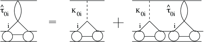
Figure 8: The equation for the pseudo two-body operator ${\hat{\tau}}_{0i}$ which is the relativistic analogue of the Watson $\tau_{0i}$ operator in the non-relativistic theory.

Now we compare $\langle\phi_{0}|{\hat{\tau}}|\phi_{0}\rangle$ and $\langle\phi_{0}|{\hat{t}^{\rm\,free}}|\phi_{0}\rangle$. Of course the difference between ${\hat{\tau}}_{0i}$ and ${\hat{t}^{\rm\,free}}_{0i}$ is the nuclear medium modification of the interaction. But for intermediate and high energies where the impulse approximation is good, the difference is not significant. One contribution arising from medium modification is the shift in the energy of the terms in the kernel due to the motion of the $A-1$ cluster. The second difference is in the iterated intermediate states where $\langle\phi_{0}|{\hat{\tau}}|\phi_{0}\rangle$ includes excited target intermediate states because of the propagator $QG_{0}Q$ in $\hat{\tau}$. In order to see what is involved in approximating $\langle\phi_{0}|{\hat{\tau}}|\phi_{0}\rangle$ by $\langle\phi_{0}|{\hat{t}^{\rm\,free}}|\phi_{0}\rangle$ we rewrite the optical potential in terms of $\hat{t}^{\rm\,free}$,

$$U = \sum\limits_{i=1}^{A}{\hat{t}^{\rm\,free}}_{0i}+\sum\limits_{i=1}^{A}{\hat{t}^{\rm\,free}}_{0i}(QG_{0}Q-{\hat{g}}){\hat{t}^{\rm\,free}}_{0i}+\cdots$$ (65)

$$+\sum\limits_{i=1}^{A}{\hat{t}^{\rm\,free}}_{0i}QG_{0}Q\sum\limits_{j\neq i}^{A}{\hat{t}^{\rm\,free}}_{0j}+\cdots$$

$$+\sum\limits_{i=1}^{A}{f}_{0i}+\sum\limits_{i=1}^{A}{f}_{0i}QG_{0}Q\sum\limits_{j\neq i}^{A}{\hat{t}^{\rm\,free}}_{0j}+\cdots$$

Compare to the non-relativistic expression (51). In equation (65) the first term in the series $\sum\limits_{i=1}^{A}{\hat{t}^{\rm\,free}}_{0i}$ when sandwiched between the target ground states will give the first-order single scattering optical potential in the impulse approximation. The second term in the series is the propagator correction term. In the non-relativistic theories, the name Impulse Approximation comes from the fact that in medium and higher energies $\langle\phi_{0}|t_{0i}QG_{0}Qt_{0i}|\phi_{0}\rangle$ can be approximated well by $\langle\phi_{0}|t_{0i}gt_{0i}|\phi_{0}\rangle$ where $g$ is the free two-body propagator. Obviously this will be a good approximation if $\langle\phi_{0}|t_{0i}QG_{0}Qt_{0i}|\phi_{0}\rangle$ is dominated by single nucleon knockout terms shown in Figure 9.

Figure 9: For medium energies one nucleon knockout terms such as this dominate and the difference between $\tau_{0i}QG_{0}Q\tau_{0i}$ and $t_{0i}QG_{0}Qt_{0i}$ is small.

The second line in the above series (65) are the double, triple, etc. scattering terms. Non-relativistically the first term plus the double scattering term constitute the second-order optical potential in the impulse approximation.

Diagrams 7e , 7f and other similar diagrams can be understood as three-body and multi-nucleon force terms in the nonrelativistic theory. Although it is possible to include them formerly in our two-body t-matrix, in order to see the OBE contribution and these multi-nucleon force terms separately, we lump all these non-OBE contributions in the $f_{0i}$ terms in equation (59) and equation (65). We will leave the labor of estimating the sizes and effects of these terms to future work. In any case, in order to obtain an RMST whose leading term is given by an OBE $t$-matrix, we do not include them in the kernel of ${\hat{\tau}}_{0i}$.

3.3 3-dimensional reduction

The Bethe-Salpeter equation (52) can be reduced from 4 to 3 dimensions by writing it as a set of coupled equations

$$T = K+K\widetilde{G}_{0}T$$ (66)

$$K = V+V(G_{0}-\widetilde{G}_{0})K$$ (67)

where $\widetilde{G}_{0}$ is a 3-dimensional propagator, which may be written in the general form [20]

$$\widetilde{G}_{0}=-2\pi i\int\frac{ds^{\prime}}{s-s^{\prime}+i\eta}\,f(s^{\prime},s)\,\delta^{+}(A)\,\delta^{+}(B)$$ (68)

where $s$ is the square of the total 4-momentum and $f(s^{\prime},s)$ is a function with the requirement that $f(s,s)=1$. $A$ and $B$ are arguments of the delta function which depend on 4-momentum [20]. These $\delta$ functions are such that they fix a prescription for first component of 4-momentum, $k_{0}$, and thereby kill a $\int dk_{0}$ integral reducing the problem from 4 to 3-dimensions. This procedure is called a 3-dimensional reduction of the Bethe-Salpeter equation, resulting in the 3-dimensional equation (66). There are infinitely many three-dimensional reductions possible [21]. The reduction is done by using some delta functions and the equations obtained by this method are commonly known as quasi-potential equations. Besides the quasi-potential equations, there exist other covariant three-dimensional equations designed to obey certain principles. For example, Phillips and Wallace have developed an equation which satisfies gauge invariance to any desired order in the kernel [22]. Pascalutsa and Tjon have designed an equation satisfying charge conjugation [23]. More details can be found in reference [20].

So far the formulation of our RMST is entirely in four dimensions and no dimensional reduction has been made. In the four-dimensional formalism, the propagator for the elastic scattering equation (55), is $PG_{0}P$ where $G_{0}$ is the Bethe-Salpeter propagator for the nucleon-nucleus system and $PG_{0}P$ tells us that the target is propagating in its ground state. Apparently the nucleon-nucleus scattering calculation has never been done in full four dimensions. In actual calculations, for proton-nucleus scattering, a fixed energy Dirac equation is used with scalar and vector potentials calculated from the $t\rho$ approximation of the optical potential. Thus one has made the assumption that the interaction is instantaneous. This means the target is infinitely heavy and the projectile moves in the instantaneous potential of the target nucleus because a fixed energy Dirac equation is a three-dimensional one-body equation. That means in using the Dirac equation, one has made two approximations. First, the Bethe-Salpeter propagator of the nucleon-nucleus system is replaced by some three-dimensional two-body propagator. Second, a proper one-body limit of the chosen three-dimensional two-body propagator is the Dirac propagator. To see what is involved, rewrite (55) and (56) as the coupled integral equations,

$$T = {\widetilde{U}}+{\widetilde{U}}P{\widetilde{G}}_{0}PT$$ (69)

$${\widetilde{U}} = U+U(PG_{0}P-P{\widetilde{G}}_{0}P){\widetilde{U}}$$ (70)

Obviously the difficulty level in solving for $\widetilde{U}$ is the same as solving the original 4-dimensional problem. In order to obtain a 3-dimensional elastic scattering equation, we choose a 3-dimensional propagator $P{\widetilde{G}}_{0}P$. All that is required to maintain unitarity is that $P{\widetilde{G}}_{0}P$ has the same elastic cut as $PG_{0}P$. Of course in picking ${\widetilde{G}}_{0}$ we must specify how the nucleon-nucleus relative energy variable is going to be handled so that equation (69) will be a three-dimensional equation. It should be clear that the relative energy prescription is entirely contained in ${\widetilde{G}}_{0}$ and $P{\widetilde{G}}_{0}P$ just tells us that the target is propagating in its ground state. Once the 3-dimensional propagator ${\widetilde{G}}_{0}$ is chosen, we have to use the same prescription for fixing the relative energy in evaluating $U$. In the nucleon-nucleus case, $U=\sum\limits_{i}{\hat{t}^{\rm\,free}}_{0i}$ contains $\hat{t}^{\rm\,free}$ whose propagator $\hat{g}$ is the Bethe-Salpeter propagator of the projectile and a target nucleon. An important conclusion of the present paper, is that to be consistent one must use the same prescription in fixing the relative energy in $G_{0}$ and $\hat{g}$. For example, in nucleon-nucleus scattering, if we are going to use a nucleon-nucleon $t$-matrix using the Blackenbeclar-Sugar propagator, the elastic scattering equation should also be the Blackenbeclar-Sugar equation.

The final elastic scattering equation need not be a Dirac equation. Making it a Dirac equation involves the assumption that the target nucleus is infinitely heavy and that the proper one-body limit of the equation corresponding to the three-dimensional equation with the propagator $P{\widetilde{G}}_{0}P$ is the Dirac equation. In reality no nucleus is infinitely heavy although it can be a good approximation for many heavy nuclei. We note also that the correct one-body limit can be easily incorporated in quasi-potential (three-dimensional) or other types of two-body equations [23].

In the case of meson projectiles, there are three different masses involved; the mass of the meson, the mass of the nucleon and the mass of the nucleus. Because of the mass difference between the meson and the nucleon, it is not suitable to use 3-dimensional quasi-potential equations which put both particles equally on mass-shell and it is also not entirely justifiable to put the nucleon on-mass-shell since the nucleon is not infinitely massive. In our opinion, the most suitable 3-dimensional equation to use for the meson-nucleon amplitude is the Proportionally Off-Mass-Shell equation [20]. The propagator of this equation can be easily modified for boson-fermion or fermion-fermion cases so it can be used for both the nucleon-nucleon and the nucleon-nucleus propagators. The major advantage of this equation over other quasi-potential equations is that it adjusts the off-shellness of the particles according to their masses. When one of the particles is infinitely massive, it reduces to a one-body equation and if the masses are equal, it treats the particles symmetrically and it reduces to an equation known as the Todorov equation [24]. Obviously, this propagator can be used for both mesonic and nucleonic projectiles and also for the projectile-taget propagation. It also gives us the added advantage that it automatically adjusts itself to the masses involved because of the physically meaningful prescription for fixing the relative energy. It would be interesting to see the use of this proportionally off-mass-shell equation in nucleon-nucleus scattering in the future.

4 Conclusions

We have formulated a relativisitic multiple scattering series for the optical potential in the the case of nucleon-nucleus scattering. As in reference [8] we started from the fact that the nucleon-nucleus scattering amplitude is given by an infinite series of meson exchange diagrams between the projectile and the target. This infinite series can be written as an integral equation (Bethe-Salpeter equation) if we include all projectile-target irreducible diagrams in the kernel. In contrast to reference [8] we do not consider the cancellation of the box and the crossed box diagrams, but derived a multiple scattering series without making any dimensional reduction. In the full 4-dimensional formalism, neither the projectile nor the target is put on-mass-shell and we do not have the problem of spurious singularities arising from putting an excited target on-mass-shell. As expected, the RMST for the optical potential is very similar to the non-relativistic counterpart. The only difference is the appearence of some extra terms arising from diagrams with the projectile interacting with two or more nucleons via meson exchange. We show that just like the non-relativistic case, the single scattering first-order impulse approximation optical potential operator is given by the free two-body Bethe-Salpeter $t$-matrix summed over the target nucleon index.

In this paper we discussed how to formulate a relativistic multiple scattering theory for the optical potential in projectile-nucleus scattering. We did not discuss about target recoil or the center of mass motion of the A-body target. In practical calculations these things have to be taken into account. One way to incorporate the A-body center of mass motion is to use the Moller frame transformation factor [25]. Mutiplying the nucleon-nucleon t-matrix (calculated in the nucleon-nucleon center of mass frame) by this factor will produce the t-matrix to be used appropriate for the nucleon-nucleus center of mass frame. In the optimal factorization of the optical potential, recoil of the struck nucleon can be taken into account by including a $-({\bf p}+{\bf p^{\prime}})/2A$ term in the struck nucleon momenta where ${\bf p}$ and ${\bf p^{\prime}}$ are the initial and final momentum in the nucleon-nucleus center of mass frame and A is the mass number of the target nucleus [26]. An in depth analysis of the effects of including boost, recoil, Moller factor and Wigner rotation in proton-nucleus scattering can be found in a study by Tjon and Wallace [26].

We have discussed that there are many possible ways to organize the relativistic multiple scattering theory. Indeed, unlike the non-relativistic case, the relativistic case already has a kernel that includes multiple scattering at the level of meson exchange. One could in principle obtain a multiple scattering series which has the exact same form as the non-relativistic case (Eq. 45) by including these $f_{0}i$ diagrams in the definition of ${\hat{\tau}}_{0i}$. This shows that one can obtain a relativistic multiple scattering series for the optical potential in the mold of the non-relativistic theory. As far as we are aware, all relativistic nucleon-nucleus scattering calculations that use a two-body t-matrix calculated from a two-body relativistic equation have used OBE models. Therefore we keep the OBE contribution and contributions from the many-body force diagrams separate so that we can see what is left out in these calculations. In this paper we try to stay close to the non-relativisitc Watson formalism. In the literature on the non-relativistic multiple scattering theory there are other ways to organize the multiple scattering series [27, 28, 29]. Developing such organizations are beyond the scope of this work.

Throughout the paper, we have illustrated our technique by separating off the OBE term shown in Figure 7a. We have mentioned several times that this particular separation is not necessary, and we have discussed how to choose alternatives. The use of the OBE term alone might be a popular choice and our discussion shows what approximations are involved in making such a choice and what terms are left out.

Next we rewrote the elastic scattering equation into coupled integral equations by introducing an auxilary interaction $\widetilde{U}$ and a propagator $P{\widetilde{G}}_{0}P$. This propagator contains a prescription for fixing the relative energy variable and must also have the same elastic cut as $PG_{0}P$ so that it will obey unitarity. The final elastic scattering equation is $T={\widetilde{U}}+{\widetilde{U}}P{\widetilde{G}}_{0}PT$ which is a three-dimensional covariant equation. The 3-dimensional optical potential $\widetilde{U}$ is obtained from $U$ by using the same relative energy prescription as in $P{\widetilde{G}}_{0}P$. This requires that the free two-body $t$-matrix in the optical potential should be calculated with the same relative energy prescription. To give a concrete example, if $P{\widetilde{G}}_{0}P$ corresponds to Blackenbeclar-Sugar propagator, then the first order impulse approximation optical optential is $\sum\limits_{i}{\hat{t}^{\rm\,free}}_{i}$ where ${\hat{t}^{\rm\,free}}_{i}$ must be calculated from the Blackenbeclar-Sugar equation. An important conclusion of this paper is that the propagators of the elastic scattering equation and the free two-body $t$-matrix must be consistent. Next, we have looked at what approximation is involved in using a fixed energy Dirac equation. Obviously, from the discussion above the final projectile-target elastic scattering equation does not have to be a Dirac equation. Since the fixed energy Dirac equation is a one-body equation, the use of it implies that the target is infinitely heavy. The more subtle point involved here is that, in doing so, we are also assuming that the correct one-body limit of the elastic scattering two-body equation with propagator $P{\widetilde{G}}_{0}P$ is a Dirac equation. The effects of other propagators other than Dirac should be tested in future calculations, although we believe that for heavy target nuclei such as ⁴⁰Ca or ²⁰⁸Pb, Dirac RIA would be an excellent approximation, Finally, we argued that it is physically more meaningful and aesthetically pleasing to use the Proportionally Off-Mass-Shell propagator [20] for projectile-nucleon and nucleon-nucleus propagators regardless of whether the projectile is a meson or a nucleon.

Acknowledgements: KMM and TC would like to acknowledge the support of COSM, NSF Coorperative Agreement PHY-0114343 and Hampton University where part of this work was done. JWN was supported by NASA grant NNL05AA05G.

References

References

- [1] Arnold L G, Clark B C, Mercer R L and Schwandt P 1981 Phys. Rev. C 43 1949; Clark B C , Hama S and Mercer R L 1982 in The Interaction Bewteen Medium Energy Nucleons in Nuclei, edited by Meyer H O, AIP Conf. Proc. No. 97 (American Institute of Physics, New York, 1983) p. 260.
- [2] McNeil J A, Shepard J R and Wallace S J 1983 Phys. Rev. Lett. 50 1439; Shepard J R, McNeil J A and Wallace S J 1983 Phys. Rev. Lett. 50 1443
- [3] Clark B C, Hama S, Mercer R L, Ray L and Serot B D 1983 Phys. Rev. Lett. 50 1644; Clark B C, Hama S, Mercer R L, Ray L and Hoffmann G W 1983 Phys. Rev. C28 1421; Hynes M V, Picklesimer A, Tandy P C and Thaler R M 1984 Phys. Rev. Lett. 52 978; Hynes M V, Picklesimer A, Tandy P C and Thaler R M 1985 Phys. Rev. C 31 1438; Gross F L, Maung K M, Tjon J A, Townsend L W and Wallace S J 1989 Phys. Rev. C 40 R10
- [4] Maung K M, Gross F L, Tjon J A and Wallace S J 1991 Phys. Rev. C 43 1378
- [5] Kurth Kerr L, Clark B C ,Hama S, Ray L,Hoffmann R W 2000 Prog. Theor. Phys. 103 321
- [6] Clark B C, Hama S, Kerr L J 2003 Phys. Rev. C 67 054605
- [7] Clark B C, Furnstahl R J, Kerr L J, Rusnak J, Hama S 1998 Phys. Lett. B 427 231.
- [8] Maung K M and Gross F L 1987, Bull. Am. Phys. Soc. 32 1029; Gross F and Maung K M 1989 Phys. Lett. B 229 188
- [9] Maung K M and Gross F L 1990 Phys. Rev. C 42 1681
- [10] Watson K M 1953 Phys. Rev. 89 575
- [11] Tandy P C 1986, in Relativstic dynamics and quark-nuclear physics, edited by Johnson M B and Picklesimer A (Wiley, New York)
- [12] Eisenberg J M and Koltun D S 1980, Theory of meson interactions with nuclei (Wiley, New York)
- [13] Scheck F 1983 Leptons, hadrons and nuclei (North-Holland, Amsterdam)
- [14] Maung K M 1994, J. Phys. G 20 L99
- [15] Feshbach H 1958, Ann. Phys. (N.Y.) 5, 357
- [16] Feshbach H 1962, Ann. Phys. (N.Y.) 19, 287
- [17] Francis N C and Watson K M 1953, Phys. Rev. 92, 291
- [18] Serot B D and Walecka J D 1986 Advances in Nuclear Physics Vol 16, edited by Negele J W and Voigt E, Plenum Press, New York.
- [19] Fleicher J and Tjon J 1980 Phys. Rev. C 21 87
- [20] Maung K M, Norbury J W and Kahana D E 1996 J. Phys. G 22 315
- [21] Woloshyn R M and Jackson A D 1973 Nucl. Phys. B 64 269
- [22] Phillips D R and Wallace S J 1998 Few Body Syst. 24 175
- [23] Pascalutsa V and Tjon J A 2002 Few Body Syst. Suppl. 10 105
- [24] Todorov I T 1971 Phys. Rev. D 10 2351
- [25] Moller C 1945 kgl. Danske Videnskab. Selsbak, Mat-fys. Medd. 23 1
- [26] Tjon J. A. and Wallace S. J. 1991Phys. Rev. C44 1156
- [27] Kerman A K, McManus H and Thaler R M 1959 Ann. Phys. 8 551
- [28] Siciliano E R and Thaler R M 1977 Phys. Rev. C 16 1322
- [29] Ernst D J, Longergan J T, Miller G A and Thaler R M 1977 Phys. Rev. C 16 537