On the reconstruction of a magnetosphere of pulsars nearby the light cylinder surface

Abstract

A mechanism of generation of a toroidal component of large scale magnetic field, leading to the reconstruction of the pulsar magnetospheres is presented. In order to understand twisting of magnetic field lines, we investigate kinematics of a plasma stream rotating in the pulsar magnetosphere. Studying an exact set of equations describing the behavior of relativistic plasma flows, the increment of the curvature drift instability is derived, and estimated for $1s$ pulsars. It is shown that a new parametric mechanism is very efficient and can explain rotation energy pumping in the pulsar magnetospheres.

1 Introduction

The aim of the present work is to investigate generation of a toroidal component of the magnetic field nearby the light cylinder surface (LCS) (a hypothetical surface, where the linear velocity of rotation equals the speed of light).

The work we consider in this paper is closely related to the pulsar wind problem. Studying the magnetic field of the Crab nebula, Piddington (1953) was first who has suggested the presence of a central object in the nebula, with frozen magnetic field inside. It has been supposed that rotation of the central body provokes generation of the toroidal component of magnetic field. Further investigations have shown that this kind of magnetic field characterizes magnetized star winds [Weber & Davis 1967]. These results have been generalized for relativistic flows in a region close to the LCS: [Michel 1969, Kennel et al. 1983, Kennel & Coroniti 1984, Begelman & Li 1992]. Despite success of developed models, they encounter a number of difficulties, when one attempts to extrapolate the wind back to the source: the pulsar magnetosphere. For large distances the wind is specified in the approximation: $\sigma\equiv B^{2}/(4\pi mc^{2}n\gamma)\ll 1$, where $B$ is the magnetic field induction, $m$ and $n$- the electron mass and density respectively and $\gamma$ the Lorentz factor of relativistic electrons. In this case, change of magnetic field’s configuration is defined only by plasma motion. This circumstance simplifies a possibility of analytical consideration of a plasma. But in the pulsar magnetospheres, a situation is opposite, the energy density of magnetic field exceeds by many orders of magnitude the energy density of the plasma $\sigma\gg 1$, therefore a need of consideration of this specific case is essential. Close to the light cylinder area the magnetic field drags behind itself the rotating electron-positron plasma and the question which arises is: how the magnetosphere is reconstructed nearby the light cylinder surface? It is obvious that close to this region, rigid rotation is impossible and consequently magnetic field lines must deviate, lagging behind the rotation of the pulsar. Implementing special MHD codes in a series of works [Michel & Krause-Polstorff 1984, Krause-Polstorff & Michel 1985, Smith et al. 2001] pulsar wind physics has been numerically studied and improved by Spitkovski & Arons (2002) and Spitkovski (2003) where plasma dynamics in 3D was presented and it has been shown that the flow goes through the LCS into the wind zone. In these papers a principal assumption is the current generated by the electric drift: $\overrightarrow{V_{E}}=c\overrightarrow{E}\times\overrightarrow{B}/B^{2}$ [Blandford 2002]. Obviously for a plasma composed of equal numbers of positive and negative charges, the current is not generated (the electric drift does not ”feel” charges), although for the pulsar plasma a primary electron beam is composed of only electrons and therefore the electric drift generates the current, leading to creation of electromagnetic fields.

In [Rogava et al. 2003] a particle moving along a curved rotating channel has been considered and it was shown that for a certain shape of curved trajectories one may avoid the light cylinder problem. Therefore one has to understand what is a mechanism responsible for the process of twisting of field lines when the condition $\sigma\gg 1$ is satisfied.

According to observations it is clear that the energy of emission is very high. An observed pulsar luminosity lies in the range: $[10^{31}-10^{38}]erg/s$ [Tores & Nuza 2002], on the other hand the only source of pulsar radiation can be rotational energy $I\omega^{2}/2$, where $I$ is moment of inertia of the pulsar, and $\omega$ - the angular velocity of rotation. As observations show the spin down luminosity is of the same order of magnitude as the radiation luminosity, therefore it is reasonable to suppose that all pulsars emit due to rotation energy decrease [Sturrock 1970]. The problem concerns the question: how the rotation energy is transformed into pulsar radiation. According to standard models, due to electric field, the charged particles uproot from a surface of the neutron star and accelerate by the electric force which results in the radiation process. The origin of this emission is supposed to be in the magnetosphere of pulsars. These models introduce a vacuum gap, inside of which the particles experience strong electric field and accelerate. But the problem arises concerning the gap size which turns out to be not enough for energy gain of charged particles [Ruderman & Sutherland 1975].

In order to resolve this problem and enlarge the gap size (which will provide increase of an acceleration length scale) many attempts have been done, applying different approaches: [Arons & Sharleman 1979, Muslimov & Tsygan 1992, Ruderman & Sutherland 1975], but no approach was able to get the efficient acceleration enough for producing observed radiation.

A new mechanism of acceleration has been introduced in [Machabeli & Rogava 1994] where a bead moving inside a straight rigidly rotating pipe has been studied. It was shown that the centrifugal force can be very efficient and if one applies this method for the pulsar magnetospheres it will provide high Lorentz factors of particles. Therefore the amount of energy contained within the $e^{+}e^{-}$ plasma is very high. If one finds mechanisms for the conversion of at least a small fraction of this energy into the variety of waves or instabilities - one might witness a number of well-pronounced and bona fide observational signatures in the pulsar radiation theory. In [Machabeli & Rogava 1994] it has been found that the radial component of velocity for relativistic particles behaves in time as $c\cos(\Omega t)$ ($c$ is the speed of light), which gives a possibility of parametric energy pumping from the mean flow into instabilities (see [Machabeli et al. 2005]). In [Machabeli et al. 2005] the $e^{+}e^{-}$ plasma has been studied and the increment of an instability of the Lengmuire waves was estimated. It has been demonstrated that the centrifugal acceleration might have been efficient enough for the observed spin down luminosity. We have shown that the linear stage was so efficient that it was very short in time, and nonlinearities were turned in soon.

In the present paper we generalize the previous work and study the parametric mechanism of the curvature drift instability driven by the centrifugal acceleration. We consider a two component plasma: a) the basic plasma flow (bulk flow) with the concentration $n_{pl}$ and the Lorentz factor $\gamma_{pl}$ and b) the beam component with the concentration $n_{b}$ and the Lorentz factor $\gamma_{b}$. It is known that in the pulsar magnetosphere the drift velocity is to be important for plasma dynamics. The drift velocity may influence processes in the plasma and especially may affect an evolution of instabilities. Unlike [Spitkovsky & Arons 2002, Spitkovsky 2003] where the processes are considered nearby the pulsar surface, in the present paper we investigate instabilities close to the light cylinder area, where effects of centrifugal acceleration should be extremely efficient. In [Spitkovsky 2003] it has been noted that the structure of pulsar magnetospheres could not be solved analytically, whereas in the present paper, we show that an initial stage of the reconstruction process of magnetospheres can be considered analytically, starting by appropriate initial conditions. Another difference is that in our model we study a plasma, which is bound by rigidly rotating straight magnetic field and the force free condition applied in [Spitkovsky & Arons 2002, Spitkovsky 2003] is not valid, because as it is shown in [Shapakidze et al. 2000] the force free condition can be provided only if the magnetic field has a configuration similar to the one of a differentially rotating Couette flow. The principally different assumption in the present paper is that instead of considering the electric drift, we study the curvature drift investigating the possibility of generation of the toroidal component $B_{r}$, which is a key step in understanding the reconstruction of the pulsar magnetosphere nearby the LCS.

The work is organized as follows. In §2 we derive the dispersion relation, in §3 the corresponding results are present and in §4 we summarize the results.

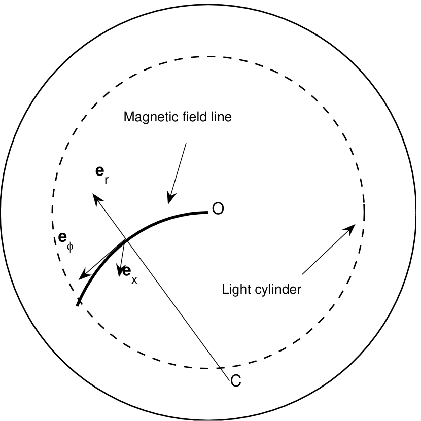
Figure 1: Here we show geometry in which we consider our system of equations. By ${\bf e_{\phi}}$, ${\bf e_{r}}$ and ${\bf e_{x}}$ unit vectors are denoted, note that ${\bf e_{x}}\perp{\bf e_{r,\phi}}$. $C$ is the curvature center.

2 Theory

Throughout the work it is supposed, that magnetic field lines are almost straight and due to the frozen-in condition the plasma particles follow the magnetic lines and accelerate. Geometry in which we consider the problem is shown in Fig. 1 [Lyutikov et al. 1999].

Our system is governed by the Euler equation [Machabeli et al. 2005]:

$$\frac{\partial{\bf p_{i}}}{\partial t}+({\bf v_{i}\nabla)p_{i}}=-\gamma\alpha{\bf\nabla}\alpha+\frac{e}{m}\left(\bf E+\bf v_{i}\times\bf B\right),$$ (1)

$$i=pl,b,$$

the continuity equation:

$$\frac{\partial n_{i}}{\partial t}+{\bf\nabla}(n_{i}{\bf v_{i}})=0,$$ (2)

and the induction equation, which closes the system:

$${\bf\nabla\times B}=\frac{1}{c}\frac{\partial{\bf E}}{\partial t}+\frac{4\pi}{c}\sum_{i=pl,b}{\bf J_{i}},$$ (3)

where ${\bf J_{i}}$ ($i=pl,b$) is the current of plasma and beam components.

We start our analysis by introducing small deviations around the equilibrium state:

$$\Psi\approx\Psi^{0}+\Psi^{1},$$ (4)

where $\Psi=(n,{\bf v},{\bf p},{\bf E},{\bf B})$.

Since we are interested in the generation of the toroidal component of magnetic field, it is interesting to study the curvature drift wave (when $\omega\sim ku_{x}$), because it is characterized by the following conditions: $B_{r}\gg B_{\phi}$, $E_{\phi}\gg E_{r}$ [Kazbegi et al. 1991] that show an importance of $B_{r}$ on the one hand and closes the system by the second condition on the other hand.

We consider the equilibrium state with a drift velocity along the $x$-axis

$$u_{0x}=\frac{\gamma v_{0\phi}^{2}}{\omega_{B}R_{B}}.$$ (5)

where $\gamma$ is the Lorentz factor, $\omega_{B}=eB_{0}/(m_{e}c)$ and $R_{B}$ is the curvature radius of the magnetic field lines ($e$ and $m$ are the charge and mass of electron and $B_{0}$-the magnetic induction). Along $\phi$, due to the centrifugal acceleration one has a relativistic flow with the velocity [Machabeli & Rogava 1994]:

$$v_{0\phi}=c\cos(\Omega t).$$ (6)

If one expresses the perturbation of physical quantities by following:

$$\Psi^{1}(t,{\bf r})\propto\Psi^{1}(t)\exp\left[i\left({\bf kr}\right)\right]\,,$$ (7)

then considering only $x$ components of the Euler and induction equation, it is easy to show that for curvature drift waves, propagating perpendicular to magnetic filed lines ($k_{\phi}\ll k_{x}$), Eqs. (1,2,3) can be reduced into the form:

$$\frac{\partial p^{1}_{ix}}{\partial t}-i(k_{x}u_{0x}+k_{\phi}u_{0\phi})p^{1}_{ix}=\frac{e}{c}v_{0\phi}B^{1}_{r},$$ (8)

$$\frac{\partial n^{1}_{i}}{\partial t}-i(k_{x}u_{0x}+k_{\phi}u_{0\phi})n^{1}_{i}=ik_{x}n_{i0}v^{1}_{x},$$ (9)

$$-ik_{\phi}cB^{1}_{r}=4\pi e\sum_{i=pl,b}(n_{i0}v^{1}_{ix}+n^{1}_{i}v_{i0x}).$$ (10)

In Eq. (8) we have used an approximate expression of velocity along the $r$-axis: $v^{1}_{r}\approx cE^{1}_{x}/B_{0\phi}$. If we choose $p^{1}_{ix}$ and $n^{1}_{i}$ to have the form:

$$v^{1}_{ix}\equiv V_{ix}e^{i{\bf kA_{i}}(t)},$$ (11)

$$n^{1}_{i}\equiv N_{i}e^{i{\bf kA_{i}}(t)},$$ (12)

where

$$A_{x}(t)=\frac{U_{ix}t}{2}+\frac{U_{ix}}{4\Omega}\sin(2\Omega t),$$ (13)

$$A_{\phi}(t)=\frac{c}{\Omega}\sin(\Omega t),$$ (14)

$$U_{ix}=\frac{c^{2}\gamma_{i0}}{\omega_{B}R_{B}},$$ (15)

then one obtains from Eqs. (8,9):

$$v^{1}_{ix}=\frac{e}{m\gamma_{i0}}e^{i{\bf kA_{i}}(t)}\int^{t}e^{-i{\bf kA_{i}}(t^{\prime})}v_{0\phi}(t^{\prime})B_{r}(t^{\prime})dt^{\prime},$$ (16)

$$n^{1}_{i}=\frac{ien_{0ik_{x}}}{m\gamma_{i0}}e^{i{\bf kA_{i}}(t)}\int^{t}dt^{\prime}\int^{t^{\prime\prime}}e^{-i{\bf kA_{i}}(t^{\prime\prime})}v_{0\phi}(t^{\prime\prime})B_{r}(t^{\prime\prime})dt^{\prime\prime}.$$

(17)

Substituting Eqs. (16,17) into Eq. (10) it reduces to the form:

$$-ik_{\phi}cB^{1}_{r}(t)=\sum_{i=pl,b}\frac{\omega^{2}_{i}}{\gamma_{i0}}e^{i{\bf kA_{i}}(t)}\int^{t}e^{-i{\bf kA_{i}}(t^{\prime})}v_{0\phi}(t^{\prime})B_{r}(t^{\prime})dt^{\prime}+$$

$$i\sum_{i=pl,b}\frac{\omega^{2}_{i}}{\gamma_{i0}}k_{x}u_{0ix}e^{i{\bf kA_{i}}(t)}\int^{t}dt^{\prime}\int^{t^{\prime\prime}}e^{-i{\bf kA_{i}}(t^{\prime\prime})}v_{0\phi}(t^{\prime\prime})B_{r}(t^{\prime\prime})dt^{\prime\prime},$$

(18)

where $\omega_{i}=\sqrt{4\pi n_{i0}e^{2}/m}$ is the plasma frequency. In order to solve this equation one has to take the Fourier time transform. For this reason if one uses the following identity:

$$e^{\pm ix\sin\Omega t}=\sum_{s}J_{s}(x)e^{\pm is\Omega t},$$ (19)

one can reduce Eq. (18):

$$B_{r}(\omega)=-\sum_{i=pl,b}\frac{\omega^{2}_{i}}{2\gamma_{i0}k_{\phi}c}\sum_{\sigma=\pm 1}\sum_{s,n,l,p}\frac{J_{s}(g_{i})J_{n}(h)J_{l}(g_{i})J_{p}(h)}{\omega+\frac{k_{x}U_{ix}}{2}+\Omega(2s+n)}\times$$

$$\times B_{r}\left(\omega+\Omega\left(2[s-l]+n-p+\sigma\right)\right)\left[1-\frac{k_{x}U_{ix}}{\omega+\frac{k_{x}U_{ix}}{2}+\Omega(2s+n)}\right]$$

$$+\sum_{i=pl,b}\frac{\omega^{2}_{i}k_{x}U_{ix}}{4\gamma_{i0}k_{\phi}c}\sum_{\sigma,\mu=\pm 1}\sum_{s,n,l,p}\frac{J_{s}(g_{i})J_{n}(h)J_{l}(g_{i})J_{p}(h)}{\left(\omega+\frac{k_{x}U_{ix}}{2}+\Omega(2[s+\mu]+n)\right)^{2}}\times$$

$$\times B_{r}\left(\omega+\Omega\left(2[s-l+\mu]+n-p+\sigma\right)\right),$$ (20)

where

$$g_{i}=\frac{k_{x}U_{ix}}{4\Omega},$$

$$h=\frac{k_{\phi}c}{\Omega}.$$

3 Discussion

One can see from the dispersion relation that the system is characterized by two different kinds of resonance, which come from the first and second terms of the right hand side of Eq. ( 20):

$$\omega+\frac{k_{x}U_{ix}}{2}+\Omega(2s+n)\simeq 0$$ (21)

and

$$\omega+\frac{k_{x}U_{ix}}{2}+\Omega(2[s+\mu]+n)\simeq 0,$$ (22)

$$s,n=\{0,\pm 1,\pm 2...\},$$

$$\mu=\pm 1.$$

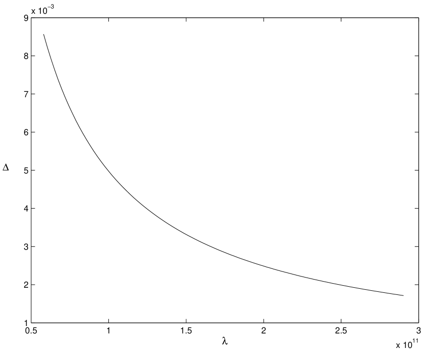
Figure 2: Dependence of the increment on $\lambda$ nearby the LCS. The set of parameters is $P=1s$, $\gamma_{b}\sim 10^{8}$, $\lambda_{\phi}=1000R_{lc}$.

As we will see later, a resonance frequency from the first condition Eq. (21) does not influence the corresponding resonance from the second expression, because if the first term is valid, the second condition is not satisfied and vice versa, when the second resonance works, the first one is not valid.

Since we are studying the mechanism of energy pumping from pulsar’s rotation and a natural consequence, that magnetic field lines must be twisted nearby the light cylinder and the twist should have a direction opposite to the rotation, one can suppose that a frequency responsible for this process must be small compared the angular velocity of the pulsar. On the other hand, assuming $\lambda\sim 6\times 10^{10}-3\times 10^{11}cm$ (where $\lambda\approx\lambda_{x}$ is the wave length) for second pulsars it is straightforward to check that $|k_{x}U_{ix}/2|\sim 0.02-0.1$, which for any values of $s$ and $n$ is much less than $\Omega(2s+n)$ for $s,n\neq 0$ (see Eq.21). Thus the only possibility which provides low frequency waves from the first resonance condition is:

$$2s+n=0.$$ (23)

Here we have assumed that $R_{B}\sim R_{p}\sim 10^{6}cm$ ($R_{p}$ is the pulsar radius). Unlike this case, second resonance condition does not provide low frequencies (see Eq.(22)), because even for vanishing $s$ and $n$, $\mu$ is not vanishing and hence it does not contribute in the process of magnetic field line’s twisting.

Let us consider the dispersion relation near the beam resonant condition expressed by Eq. (21). Then only resonant terms will be preserved and Eq. (20) will reduce:

$$B_{r}(\omega_{0})\approx-\frac{\omega^{2}_{b}k_{x}U_{bx}}{2\gamma_{b0}k_{\phi}c}\sum_{\sigma=\pm 1}\sum_{s,l,p}\frac{J_{s}(g_{b})J_{-2s}(h)J_{l}(g_{b})J_{p}(h)}{\widetilde{\Delta}^{2}}\times$$

$$\times B_{r}\left(\omega_{0}+\Omega\left(-2l-p+\sigma\right)\right),$$ (24)

where

$$\omega_{0}\approx-\frac{k_{x}U_{bx}}{2}$$ (25)

and the frequency has been expressed by the form:

$$\omega\equiv\omega_{0}+i\widetilde{\Delta}.$$ (26)

Here $\widetilde{\Delta}$’s imaginary part $\Delta\equiv Im(\widetilde{\Delta})$ is related to the increment of the instability. Since a dominant term in Eq. (24) comes from low frequencies ($\omega_{0}\ll\Omega$), then the only terms contributed in a time average will have $p$ equal to $\Omega(2(s-l)+n+\sigma)$, because all other terms with $B_{r}(\omega_{0}+\Omega q)$ ($q\neq 0$) give zero due to an oscillative character with very big values of frequencies. Taking into account this condition, one gets:

$$B_{r}(\omega_{0})\approx-\frac{\omega^{2}_{b}k_{x}U_{bx}}{2\gamma_{b0}k_{\phi}c}\sum_{\sigma=\pm 1}\sum_{s,l}\frac{J_{s}(g_{b})J_{-2s}(h)J_{l}(g_{b})J_{-2l+\sigma}(h)}{\Delta^{2}}\times$$

$$\times B_{r}(\omega_{0}).$$ (27)

From here one can easily express the increment by following:

$$\Delta\approx\left[-\frac{\omega^{2}_{b}k_{x}U_{bx}}{2\gamma_{b0}k_{\phi}c}\Sigma_{1}(g_{b},h)\Sigma_{2}(g_{b},h)\right]^{\frac{1}{2}},$$ (28)

where

$$\Sigma_{1}(g_{b},h)\equiv\sum_{s}J_{s}(g_{b})J_{-2s}(h),$$ (29)

$$\Sigma_{2}(g_{b},h)\equiv\sum_{\sigma=\pm 1}\sum_{l}J_{l}(g_{b})J_{-2l+\sigma}(h).$$ (30)

Strictly speaking $\Sigma_{1}$ and $\Sigma_{2}$ are functions of $g_{b}$ and $h$ and one can show, that these summations are convergent (see Appendix).

It is interesting to investigate the increment versus following physical quantities: $\lambda_{x}$ (for the fixed, and very big in comparison with $\lambda_{x}$ values of $\lambda_{\phi}$). On the other hand one has to compare results with an observational evidence. As we have already mentioned the only source that may provide energy for radiation is the slowdown of the pulsar: $\dot{W}\approx I\Omega\dot{\Omega}$, here $I$ is moment of inertia of the pulsar. The rate of rotation energy loss can be estimated by following ratio: $\dot{W}/W\simeq 2\dot{\Omega}/\Omega=2\dot{P}/P$, where $P$ is rotation period of the pulsar. The given ratio is different for different pulsars and ranges from $10^{-11}\sec^{-1}$ (PSR 0531) to $10^{-18}\sec^{-1}$ (PSR 1952+29). Therefore the increment of the instability must not be less than $2\dot{P}/P$.

We investigate the instability rate nearby the light cylinder, because the centrifugal acceleration should be most efficient in this region. In Fig. 2 we show dependence of the increment on: $\lambda_{x}$ nearby the LCS. The set of parameters is $P=1s$, $\gamma_{b}\sim 10^{8}$, $\lambda_{x}\approx\lambda$, $\lambda_{\phi}=1000R_{lc}$ and it is supposed that $k_{x}<0$ and $U_{bx}>0$ (otherwise the resonance frequency is unphysical - negative). Here $R_{lc}$ is the light cylinder radius. Such a choise of $\lambda_{\phi}$ provides almost perpendicular (to the equatorial plane) propagation of waves. One can see that the increment reaches the value $\sim 10^{-2}$, which is more by many orders of magnitude than typical values of $2\dot{P}/P$. The linear stage will be very efficient and short in time strongly indicating the non linear regime of the phenomenon. A need of non linear saturation is seen also from the fact that $B_{r}$, which is responsible for twisting of magnetic field lines, oscillates with frequency $\omega_{0}$, due to this oscillation, $B_{r}$ not only will lag behind the rotation, which is physically reasonable, but also will advance it, therefore the need of non linear saturation of the instability increment is essential. Therefore initially created small perturbations will rapidly increase in time and thanks to the instability process, it will extract energy from the background flow into the energy of electrostatic waves.

4 Summary

1. Considering the relativistic plasma flow composed of the primary and secondary (beam) components, we have studied the role of the centrifugal acceleration in the curvature drift instability.

2. Making the linear analysis of equations, we have derived the dispersion relation and a new mechanism of the parametric instability responsible for rotation energy pumping has been found.

3. Considering low frequencies, which are responsible for twisting of magnetic field lines, an expression for the instability increment has been obtained.

4. Studying dependence of increment on $\lambda_{x}$, it has been found that the instability was very efficient and increments were more than pulsar spin down rates by many order of magnitude indicating the need of the non linear consideration of the problem.

   As we have seen, the analysis indicated the importance of the non linear stage in dynamics of the instability, therefore it is essential to study the same problem numerically by implementing a special relativistic MHD code, which will comprise one more step closer to the real scenario.

Appendix A

In this section we would like to show that the sum:

$$\Sigma_{1}(g_{b},h)\equiv\sum_{s}J_{s}(g_{b})J_{-2s}(h),$$ (31)

is finite.

In order to prove the convergence of (A.1) we use the following inequality:

$$|J_{\nu}(x)|\leq\frac{1}{\Gamma(\nu+1)}\left(\frac{x}{2}\right)^{\nu}e^{Im[x]}.$$ (32)

Here: $\nu\geq-\frac{1}{2}$.

Then for the term in $\Sigma_{1}(g_{b},h)$, one can write:

$$|J_{s}(g_{b})J_{2s}(h)|\leq\frac{1}{(s+1)!(2s+1)!}\left(\frac{g_{b}}{2}\right)^{s}\left(\frac{h}{2}\right)^{2s+1}.$$ (33)

where we have used the well known equivalence:

$$J_{-\nu}(x)=(-1)^{\nu}J_{\nu}(x).$$ (34)

This condition shows that $C_{s}\equiv|J_{s}(g_{b})J_{2s}(h)|\leq U_{s}$, where:

$$U_{s}=\frac{1}{(s+1)!(2s+1)!}\left(\frac{g_{b}}{2}\right)^{s}\left(\frac{h}{2}\right)^{2s+1}.$$ (35)

Let us prove that the $U_{s}$ is convergent using the Dalamber criterion, by introducing the following ratio:

$$\frac{U_{s+1}}{U_{s}}=\left(\frac{g_{b}}{2}\right)\left(\frac{h}{2}\right)^{2}\frac{1}{(s+2)(2s+2)(2s+3)}.$$ (36)

It is obvious that one can find $s_{0}$ for which $\frac{U_{s_{0}+1}}{U_{s_{0}}}\equiv q<1$. We see that the expression in Eq. (36) decreases with an increasing value of $s$, i.e:

$$\frac{U_{s+1}}{U_{s}}<q=\left(\frac{g_{b}}{2}\right)\left(\frac{h}{2}\right)^{2}\frac{1}{(s_{0}+2)(2s_{0}+2)(2s_{0}+3)}<1,$$ (37)

$$s\geq s_{0}.$$

This means that the sequence $U_{s}$ is convergent, and hence for $s\geq 0$ the summation $\Sigma_{1}(g_{b},h)$ is finite.

When considering the case $s<0$ and formally introducing a new index $m\equiv-s$, one obtains an expression:

$$|J_{m}(g_{b})J_{2m}(h)|,$$ (38)

similar to a corresponding term in Eq.(33) for $s\geq 0$ and hence, the summation for negative values of $s$ is also convergent.

The proof for convergence of the second summation $\Sigma_{2}(g_{b},h)$ (see Eq. (30)) does not principally differ from the one we have already considered and therefore we do not show it here.

References

- [Arons & Sharleman 1979] Arons J. & Sharleman E. T., 1979, ApJ, 231, 854
- [Begelman & Li 1992] Begelman, Mitchell C., Li Zhi-Yun, 1992, ApJ, 397, 187
- [Blandford 2002] Blandford R.D., 2002, astro-ph/0202265
- [Kazbegi et al. 1991] Kazbegi A.Z., Machabeli G.Z., Melikidze G.I., 1991, AuJPh, 44, 573
- [Kennel & Coroniti 1984] Kennel C.F. & Coroniti F.V., 1984, ApJ, 283, 710
- [Kennel et al. 1983] Kennel C.F., Fujimutra F.S., Okamoto I., 1983, GApFD, 26, 147
- [Krause-Polstorff & Michel 1985] Krause-Polstorff J. & Michel F.C. , 1985, A&A, 144, 72
- [Lyutikov et al. 1999] Lyutikov M., Machabeli G. & Blandford R., 1999, ApJ, 512, 804L
- [Machabeli et al. 2005] Machabeli G., Osmanov Z. & Mahajan, 2005, PhPl, 12, 062901
- [Machabeli & Rogava 1994] Machabeli G.Z. & Rogava A. D., 1994, Phys.Rev. A 50, 98
- [Muslimov & Tsygan 1992] Muslimov A. G. & Tsygan, 1992, MNRAS, 255, 61
- [Michel 1969] Michel F.C., 1969, ApJ, 158, 727
- [Michel & Krause-Polstorff 1984] Michel F.C. & Krause-Polstorff J., 1984, MNRAS, 213, 43
- [Piddington 1957] Piddington J.H., 1957, AuJPh, 10, 530
- [Rogava et al. 2003] Rogava, A. D., Dalakishvili, G., Osmanov Z.N., 2003, Gen. Rel. and Grav. 35, 1133
- [Ruderman & Sutherland 1975] Ruderman M. A. & Sutherland P. G., 1975, ApJ, 196, 51
- [Shapakidze et al. 2000] Machabeli G.Z., Mchedishvili G.Z. & Shapakidze D.E., 2000, Ap&SS, 271, 277
- [Smith et al. 2001] Smith I.A., Michel F.C., Thacker P.D., 2001, MNRAS, 322, 209
- [Spitkovsky & Arons 2002] Spitkovsky Anatoly & Arons Jonathan, 2002, astro-ph/0201360
- [Spitkovsky 2003] Spitkovsky Anatoly, 2003, astro-ph/0310731.
- [Sturrock 1970] Sturrock P.A., 1970, ApJ, 164, 529
- [Tores & Nuza 2002] Torres Diego F., & Nuza Sebastián E. , 2002, ApJ, 583, L25
- [Weber & Davis 1967] Weber E.J. & Davis L.Jr., 1967, ApJ, 148, 217