Turbulence-induced magnetic flux asymmetry at nanoscale junctions

Abstract

It was recently predicted [J. Phys.: Condens. Matter 18, 11059 (2006)] that turbulence of the electron flow may develop at nonadiabatic nanoscale junctions under appropriate conditions. Here we show that such an effect leads to an asymmetric current-induced magnetic field on the two sides of an otherwise symmetric junction. We propose that by measuring the fluxes ensuing from these fields across two surfaces placed at the two sides of the junction would provide direct and noninvasive evidence of the transition from laminar to turbulent electron flow. The flux asymmetry is predicted to first increase, reach a maximum and then decrease with increasing current, i.e. with increasing amount of turbulence.

The hydrodynamics of the electron liquid dates back to earlier studies by Madelung, Bloch Madelung (1926); Bloch (1933) and later on by Martin and Schwinger Martin and Schwinger (1959). In this latter work, in particular, it was shown that the many-body time-dependent Schrödinger equation (TDSE) can be written exactly in hydrodynamic form in terms of the density $n({\bf r},t)$ and velocity field ${\bf v}({\bf r},t)={\bf j}({\bf r},t)/n({\bf r},t)$, the ratio of the current and charge density, with all many-body interactions lumped into a two-particle stress tensor.

In recent years, the analogy of the electron flow with classical fluid dynamics has been pushed even further with the development of time-dependent density-functional methods and the consequent realization that under certain conditions, the exchange-correlation potentials can be written in hydrodynamic form Vignale et al. (1997); Tokatly (2005). More recently, it was shown that electron flow in nanoscale constrictions satisfies the conditions to write the two-particle stress tensor in a form similar to the stress tensor of the Navier-Stokes equations with an effective viscosity of the electron liquid (see also below) D’Agosta and Di Ventra (2006). The most striking prediction of this result is that, under specific conditions on the current, density and junction geometry, the electron flow should undergo a transition from laminar to turbulent regimes. D’Agosta and Di Ventra (2006) Recently, this behavior was confirmed numerically by solving directly the TDSE within time-dependent current-density functional theory Bushong et al. (2007) and comparing the results with the generalized Navier-Stokes equations derived in Ref. D’Agosta and Di Ventra (2006). In experiments, however, detecting turbulence via direct imaging of the current density remains challenging. For instance, scanning-probe microscopy (SPM) experiments which image the current flow in a 2D electron gas (2DEG) have been reported Topinka et al. (2000). These experiments employ an SPM tip to reflect electrons back toward the junction, and measure the resultant change in the total current. This means that the image thus obtained gives the correlation between the tip position and junction current, which does not necessarily correspond to the magnitude of the current density. Moreover, SPM-type experiments necessarily disturb the electron flow at the tip position, and are therefore essentially invasive.

Another way to probe turbulence would be to measure the noise properties of the current. However, the analytical description of turbulence is a notoriously intractable problem, thus making it unclear what noise characteristics the turbulent flow of electrons would generate. In addition, this noise would necessarily correlate with other intrinsic types of noise, especially shot noise Chen and Di Ventra (2003).

In the present Letter we show that the measurement of the current-induced magnetic field at the two sides of an otherwise symmetric nanojunction provides a direct and non-invasive way of measuring the transition from laminar to turbulent flow. In particular, we predict that the fluxes ensuing from the current-induced magnetic field across two surfaces on the two sides of the junction would at first become increasingly different with increasing current. This asymmetry reaches a maximum, and then decreases with further increase of the current. The measurement of these fluxes is within reach of present experimental capabilities, and thus the observation and study of this phenomenon would provide valuable insight into the transport properties of nanoscale systems.

The structure we have in mind consists of two symmetric regions of a 2DEG connected non-adiabatically by a nanojunction (the edges of this structure are represented with solid lines in the left panel of Figs. 1 and 2). The non-adiabaticity requirement is due to the fact that, as shown in Ref. D’Agosta and Di Ventra (2006), an adiabatic constriction produces a Poiseuille flow, which is laminar for essentially all currents one can effectively inject in a 2DEG.  The lateral ($y$-direction) boundaries are closed to current flow, and the longitudinal ($x$-direction) boundaries are open, with current being injected in the “top” boundary and exiting in the “bottom” boundary. We then envision two identical surfaces – placed at a given distance from the 2DEG in the $z$ direction – across which we calculate the current-induced magnetic flux (see Fig. 1). These magnetic fluxes can be measured by two superconducting interference devices (SQUIDs) Gallop (1991) located on the two sides of the junction as illustrated in Fig. 1.

Our starting point is the time-dependent Schrödinger equation written in the approximate Navier-Stokes form for an incompressible fluid D’Agosta and Di Ventra (2006)

$$D_{t}n({\bf r},t)=0,\,\,{\bf\nabla}\cdot{\bf v}({\bf r},t)=0,$$

$$\begin{split}m^{*}n({\bf r},t)D_{t}v_{i}({\bf r},t)=&-\frac{\partial}{\partial r_{i}}P({\bf r},t)+\eta\nabla^{2}v_{i}({\bf r},t)\\ &-n({\bf r},t)\frac{\partial}{\partial r_{i}}V_{\rm ext}({\bf r},t)\end{split}$$ (1)

where $D_{t}=\frac{\partial}{\partial t}+({\bf v}\cdot{\bf\nabla})$ is the convective derivative, $m^{*}$ is the effective mass of the electrons, $n({\bf r},t)$ is the electron density, $P({\bf r},t)$ is the pressure of the electron liquid, and $V_{\rm ext}({\bf r},t)$ is the sum of the Hartree and the ionic potentials. The quantity $\eta=\hbar nf(n)$ is the viscosity of the electron liquid, with $f(n)$ a smooth function of the density. The values of the viscosity as a function of density have been calculated using linear-response theory Conti and Vignale (1999); D’Agosta et al. (2007); here, we use the 2D interpolation formula of Ref. Conti and Vignale, 1999. We also employ the jellium approximation for the electron liquid, which together with the assumption of incompressibility, allows us to neglect spatial variations of $V_{\rm ext}({\bf r},t)$. Incompressibility of the electron liquid represents to a good approximation the behavior of metallic quantum point contacts D’Agosta and Di Ventra (2006); Bushong et al. (2007).

The current density was calculated numerically as a solution of Eqs. (1) Popinet (2003) for a nanojunction 28 nm wide. We have used Dirichlet boundary conditions for the velocity at the inlet, and Neumann boundary conditions at the outlet. We use parameters corresponding to a GaAs-based 2DEG: $m^{*}=0.067m_{\rm e}$, and $n=5.13\times 10^{11}\,{\rm cm}^{-2}$. The calculations were performed at a fixed value of the total average current flowing through the system selected in the range from $0.001\,{\rm\mu A}$ to $10\,{\rm\mu A}$. The magnetic field profile was found for each calculated current density distribution. The size of the surface area across which we calculated the magnetic flux was chosen to be 200 $\times$ 200 (nm)². Each surface is displaced laterally to one side of the nanojunction as shown in Fig. 1. This surface represents the SQUID area and is within reach of current technology Lam and Tilbrook (2003), although, in principle, the SQUID’s area does not necessarily need to be so small. We assume that the surfaces are located 50 nm above the 2DEG; therefore, the distributions of magnetic field were calculated at this distance from the 2DEG. Increasing this distance by a factor of two decreases the flux by about a factor of two.  For convenience, from now on we shall call these two surfaces, SQUID 1 area and SQUID 2 area (Figs. 1 and 2).

The magnetic field fluxes allow us to characterize the degree of asymmetry in the current flow pattern as well as to probe such specific features of turbulent current flow as eddies. We find that at low currents, the electron flow pattern is symmetric (see left panel of Fig 1). More precisely, the patterns of current flow in the two electrodes are mirror images of each other, with the overall sign of the flow reversed Bushong et al. (2007). This is illustrated in the left panel of Fig. 1, where we plot the velocity distribution of the electron liquid at a simulation time of 24 ps. The total current is $0.1\,{\rm\mu A}$, which is small enough that the flow is in the laminar regime, as it is evident from the figure. In the right panel of Fig. 1, we show the $z$-component of the magnetic field through a plane 50 nm above the 2DEG. As is typical of the laminar regime, the current-induced magnetic fields above the top and bottom contacts are almost symmetric with respect to the center of the junction producing an almost symmetric flux across the areas. Hence, SQUIDs positioned as indicated in Fig. 1 would measure almost equal magnetic fluxes.

By increasing the current, the current density in the source and drain sides loses top-down symmetry: the current density in the outgoing side becomes turbulent, while the current density in the incident side remains laminar (Fig 2). We note that at large currents we observe the formation of turbulent “eddies” which evolve in time, rather than a completely chaotic current density distribution. This means that at the current values we consider here turbulence is not fully developed Bushong et al. (2007).

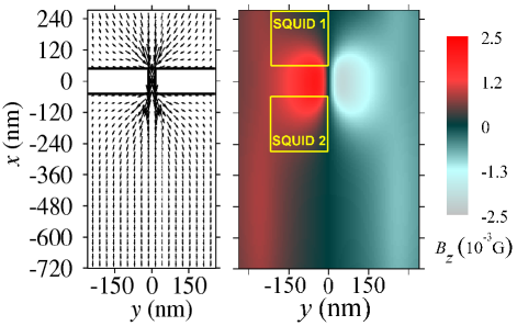
Figure 1: (Color online) Laminar current flow at a low value of the total current ($0.1\,{\rm\mu A}$). Left panel: electron velocity distribution. The arrow length is proportional to the velocity magnitude. Right panel: normal component of the magnetic field through a plane 50 nm above the 2DEG. The surface areas indicated with SQUID 1 and SQUID 2 represent two areas across which we calculate the magnetic flux (see text).

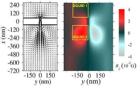
Figure 2: (Color online) Turbulent current flow at high value of the total current ($1\,{\rm\mu A}$). Left panel: electron velocity distribution. Right panel: normal component of the magnetic field through a plane 50 nm above 2DEG. The top-down symmetry in magnetic field distributions across the SQUID areas is lost. The magnetic field flux through SQUID 2 is significantly higher then the flux through SQUID 1.

Fig. 2 illustrates the behavior typical for the turbulent regime. This plot corresponds to a total current of $1.0\,{\rm\mu A}$ at time $t=24$ ps. As before, the left panel illustrates the electron velocity distribution. Unlike the electron velocity field presented in Fig. 1, the electron velocity distributions in the top and bottom electrodes in Fig. 2 are no longer symmetric. In particular, the electron velocity distribution in the bottom contact shows eddies and an increased current density in the middle of the junction. Such a velocity field is responsible for a much stronger magnetic field above the bottom contact (in particular, in the SQUID 2 area in Fig. 2). The magnetic field distribution above the top contact in Fig. 2 is “smooth” and uniform, and has a structure similar to the magnetic field distribution above the top contact of Fig. 1.

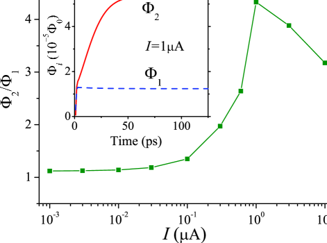
Figure 3: (Color online) Asymptotic value of the ratio of the flux through SQUID 2 area to the flux through the SQUID 1 area as a function of the total current. See text for details. Inset: Time dependence of fluxes (in units of $\Phi_{0}=h/2e$) through the top (dashed blue line) and the bottom (solid red line) SQUID areas, for a total current of $1.0\,{\rm\mu A}$.

For both the laminar and turbulent cases, as time passes, the fluxes through the top and bottom SQUID areas saturate to constant values. This is shown in the inset of Fig. 3 where we plot the flux through the top and bottom SQUID areas as a function of time for the $1.0\,{\rm\mu A}$ case. We can now determine the magnetic signature of the transition between the laminar and turbulent regimes by plotting the asymptotic value of the ratio of the magnetic fluxes through the two SQUID areas as a function of the total current. This is illustrated in Fig. 3 and shows the main findings of this paper.

At low currents (laminar regime), the current density in the top and bottom contacts is highly symmetric. Therefore, the ratio of the fluxes is near unity . There is a definite transition at the critical current $I_{c}\backsimeq 0.3\,{\rm\mu A}$, after which the ratio of the magnetic fluxes increases by more than 300%. The flux ratio reaches a maximum at a current of about $1\mu$A. Increasing the current further, we find that the flux ratio decreases. This can be explained as follows. Near the critical current, the eddies are small and stationary. These smaller, localized eddies lead to a higher ratio $\Phi_{2}/\Phi_{1}$ and the increase we observe. On the other hand, by increasing the current further, the eddies grow in size and “spread out” away from the junction thus reducing the flux ratio. Note that fully-developed turbulence would decrease the ratio $\Phi_{2}/\Phi_{1}$ even further, since eddies having clockwise and counter-clockwise senses would be continuously generated and destroyed. In addition, the noise level of modern SQUIDs Ketchen et al. (1991) is below $10^{-6}\Phi_{0}$ ( $\Phi_{0}=h/2e$ is the magnetic flux quantum), which is well below the flux magnitude shown in the inset of Fig. 3.

Figure 4: (Color online) Magnetic field correlation function, for total currents of $1.0\,{\rm\mu A}$ (solid orange curve) and $0.1\,{\rm\mu A}$ (dashed blue curve). Because the total current differs between the two by a factor of 10, we have scaled the $0.1\,{\rm\mu A}$ curve by a factor of $10^{2}$. Even after this scaling, $C_{zz}$ is significantly larger in the turbulent (high-current) case than it is in the laminar (low-current) case.

We conclude by quantifying the degree of turbulence of the current-induced magnetic field. While this cannot be directly measured, it provides insight into the properties of the turbulent regime attainable experimentally. Let us then calculate the magnetic field correlation tensor, which quantifies the spatial correlation of the magnetic field at different points in space. We define this tensor as

$$C_{ij}=\langle(B_{i}({\bf r})-B_{i}({\bf r}+\delta{\bf r}))(B_{j}({\bf r})-B_{j}({\bf r}+\delta{\bf r}))\rangle\,.$$ (2)

Here, $B_{i}$ and $B_{j}$ denote components of the magnetic field, and $\delta{\bf r}$ is a given vector. The brackets $\langle\ldots\rangle$ denote averaging over all pairs of positions separated by $\delta{\bf r}$ within a given region. Note that, even before performing a spatial average, the magnetic field already has a nonlocal character, in that the magnetic field at a point is due to the velocity of charges in the whole system.

In Fig. 4 we plot the magnetic field correlation tensor $C_{\rm zz}$, for $\delta{\bf r}=(\delta x,0)$ at $50$ nm above the 2DEG as a function of $\delta x$. The spatial averaging was carried out in a region “downstream” from the junction, in the region $x=[-487\,{\rm nm},-235\,{\rm nm}]$, $y=[0\,{\rm nm},259\,{\rm nm}]$. As expected, in the laminar case, the magnetic field varies with distance by a small amount, so that $C_{zz}$ is small. In the turbulent case, the presence of the eddies leads to a magnetic field that correlates spatially, causing $C_{zz}$ to increase with distance.

Finally, we discuss some possible alternatives to measuring turbulence via the proposed magnetic fluxes. For one, instead of using two SQUIDs placed at the two sides of the junction one could envision the use of only one SQUID, by changing the direction of current flow by merely reversing the bias. This also ensures that the effect of unavoidable scattering by defects/impurities on the magnetic fluxes is accounted for identically for both possible directions of overall current flow. Another alternative is to use a movable SQUID Kirtley et al. (1995) or scanning Hall-probe microscopy Dinner et al. (2005). In particular, if an X-Y stage were added to the apparatus, so that the substrate (or the SQUID) were movable, one could generate images of the magnetic flux as a function of position. For instance, this scanning SQUID microscopy has been previously employed to study the spatial configuration of vortices in Type II superconductors Veauvy et al. (2004). Imaging electron flow in this way would provide information about the electric current density throughout the device with the added benefit that the measurement would be noninvasive . However, we expect scanning SQUID microscopy to have a lower sensitivity due to the increased distance between the SQUID and the sample.

One can also tune the critical current value at which the transition between laminar and turbulent regimes occurs by using materials with different effective masses. For example, the heavy-hole effective mass in p-doped GaAs is about $0.45m_{e}$, which implies that the transition to turbulent flow in p-doped GaAs should occur at $I^{\prime}_{\rm c}=(0.067/0.45)*I_{\rm c}=0.047\,{\rm\mu A}$ for the same doping density as the n-doped case.

This work was supported by the U.S. Department of Energy under grant DE-FG02-05ER46204.

References

- Madelung (1926) E. Madelung, Z. Phys. 40, 322 (1926).
- Bloch (1933) F. Bloch, Z. Phys. 81, 363 (1933).
- Martin and Schwinger (1959) P. C. Martin and J. Schwinger, Phys. Rev. 115, 1342 (1959).
- Vignale et al. (1997) G. Vignale, C. A. Ullrich, and S. Conti, Phys. Rev. Lett. 79, 4878 (1997).
- Tokatly (2005) I. V. Tokatly, Phys. Rev. B 71, 165104 (2005).
- D’Agosta and Di Ventra (2006) R. D’Agosta and M. Di Ventra, J. Phys.: Condens. Matter 18, 11059 (2006).
- Bushong et al. (2007) N. Bushong, J. Gamble, and M. Di Ventra, Nano Lett. (2007), in press.
- Topinka et al. (2000) M. A. Topinka, B. J. LeRoy, S. E. J. Shaw, E. J. Heller, R. M. Westervelt, K. D. Maranowski, and A. C. Gossard, Science 289, 2323 (2000).
- Chen and Di Ventra (2003) Y. C. Chen and M. Di Ventra, Phys. Rev. B 67, 153304 (2003).
- Gallop (1991) J. C. Gallop, SQUIDS, the Josephson effects and superconducting electroncs (IOP Publishing Ltd., 1991).
- Conti and Vignale (1999) S. Conti and G. Vignale, Phys. Rev. B 60, 7966 (1999).
- D’Agosta et al. (2007) R. D’Agosta, M. Di Ventra, and G. Vignale, Phys. Rev. B (in press) (2007).
- Popinet (2003) S. Popinet, J. Comput. Phys. 190, 572 (2003).
- Lam and Tilbrook (2003) S. K. H. Lam and D. L. Tilbrook, Appl. Phys. Lett. 82, 1078 (2003).
- Ketchen et al. (1991) M. B. Ketchen, M. Bhushan, S. B. Kaplan, and W. J. Gallagher, IEEE Trans. Magn. MAG-27, 3005 (1991).
- Kirtley et al. (1995) J. R. Kirtley, M. B. Ketchen, C. C. Tsuei, J. Z. Sun, W. J. Gallagher, Lock See Yu-Jahnes, A. Gupta, K. G. Stawiasz, and S. J. Wind, IBM J. Res. Dev. 39, 655 (1995).
- Dinner et al. (2005) R. B. Dinner, M. R. Beasley, and K. A. Moler, Rev. Sci. Instrum. 76, 103702 (2005) 76, 103702 (2005).
- Veauvy et al. (2004) C. Veauvy, K. Hasselbach, and D. Mailly, Phys. Rev. B 70, 214513 (2004).
- Di Ventra and Lang (2002) M. Di Ventra and N. D. Lang, Phys. Rev. B 65, 045402 (2002).
- Sai et al. (2007) N. Sai, N. Bushong, R. Hatcher, and M. Di Ventra, Phys. Rev. B 75, 115410 (2007).
- Liu et al. (2002) J. Liu, A. Harris, and N. Kanwisher, Nat. Neurosci. 5, 910 (2002).