Geometry-induced frustration of magnetization in a planar soft-hard magnetic system

Abstract

We computationally study the frustrated magnetic configurations of a thin soft magnetic layer with the boundary condition fixed by underlying hard magnets. Driven by geometrical constraints and external magnetic field, transitions between frustrated energy minima result in magnetic hysteretic behavior. The presence of soft-magnet introduces strong undulations in the energy landscape in a length scale set by the magnetic property of the soft magnet. We propose a possible use of the phenomena to locally control the movement of magnetic nanoparticles.

Magnetic systems with geometrical frustration has attracted considerable attention for the presence of multiple ground states and intricate thermodynamics properties moessner ; schiffer for many decades. Soft-hard magnetic structures have recently been intensively investigated for their high coercivity and saturation magnetization properties  kneller ; coehoom ; zeng . Exchange-coupled planar soft-hard magnetic structures  eiichi ; sabir1 ; sabir2 ; asti show a rich variety of magnetic configurations when magnetic frustration is induced geometrically. This is particularly the case when the characteristic length of magnetization configuration is comparable to the device size.

Previous works on soft-hard magnetic systems siegmann ; rohl ; hellwig ; stamm have mostly focussed on magnetization configurations between layers of soft-hard magnets. In this paper, we study two-dimensional geometry-induced multiple magnetic configurations, its associated configurational energy minima, and external magnetic field-induced transitions between these configurations. We concentrate on the magnetization configurations in the plane of the soft magnet, determined by the magnetization directions of the constraining hard magnets and an external field.

Controlling magnetic states has a wide range of applications such as memory devices, sensors that use magnetostriction, etc. Here we focus on a magneto-mechanical application, namely, moving magnetic nanoparticles. The ability to move, confine, and rotate nanoparticles has come from creating non-uniform magnetic fields using either hard magnets or electromagnets  gosse ; devries ; yan ; trepat ; mirowski . We use geometrical frustration to create localized non-uniform magnetic fields. Physical properties of biomolecules such as tensile strength can be studied by attaching magnetic nanoparticles to them and applying force on the nanoparticles by trapping them in such localized magnetic energy minima.

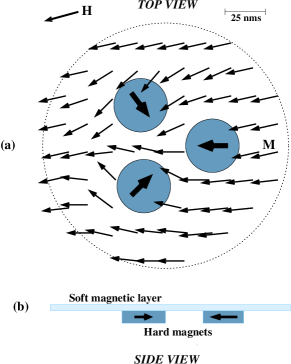
Figure 1: (a) 2-dimensional soft-hard magnetic composite system. The magnetic structure in the soft-magnetic region is determined by the boundary condition fixed by the hard magnetic discs and external field ${\bf H}$. One of possible energy minima, with two magnetic in-flux and one out-flux between the discs, is shown. (b) Side-view of the device.

The 2-dimensional soft-hard magnetic system under study consists of three hard magnetic discs placed underneath a thin soft magnetic layer (see FIG. 1). The three hard magnets, placed on vertices of an imaginary equilateral triangle, are chosen to have their magnetizations pointing toward the center of the triangle. The role of the hard magnets is to fix the magnetization boundary condition on the soft-magnet at the interface, and to introduce frustration in the system. We assume that the magnetization of the soft-magnetic layer is in-plane, and that the soft magnetic layer is thin enough ($5$ nm) that its magnetization direction varies little across the width of the layer. FIG. 1 shows one of the possible energy minimum configurations of the soft-hard magnetic system.

The energetically favorable configurations are found to be the ones where the magnetization flows in through two of the necks (region between two hard magnetic discs) which are then balanced out by the out-flux through the remaining neck. Such a configuration is shown in FIG. 1(a). Although the configuration in FIG. 1(a) is at a local energy minimum, the high energy density near the neck of out-flux due to the high gradient of magnetization makes the system unstable against external field and triggers a transition to another local minimum. Configurations only with in-flux or out-flux are highly unfavorable energetically due to the high divergence of magnetization at the center of the soft-hard magnet, but will nevertheless be reached if the system’s initial magnetization is closer to the above mentioned configurations.

Even with the magnetization restricted to be in-plane, the above-mentioned unfavorable configuration can be made stable. Introduction of a hole (or non-magnetic region) at the center of the soft magnetic disc allows magnetization to form a vortex around the hole, thereby avoiding high energy cost. The other way is to let the magnetization to point along z-direction by controlling the thickness of the magnetic layer, in which case, the energy cost of convergence will be minimized considerably, with the magnetization choosing to point in z-direction at the point of convergence. Such deviations could be utilized in devices to manipulate the softness of magnetization.

The system of FIG. 1 can be fabricated using CoCr-based alloy as hard magnetic discs and permalloy or FeCo as soft magnet. CoCr-alloy thin film can be grown by sputtering and patterned lithographically into three circular discs forming an equilateral triangle. MFM tip can be used to pin the magnetization orientation of the discs to predefined directions. Soft magnetic film can then be coated on top of the hard discs.

The equation for Hamiltonian density of the system is

$${\cal H}=\frac{J}{3A^{2}}|\nabla{\bf m}|^{2}-M_{0}^{2}{\bf m}\cdot{\bf h}+V_{0}(|{\bf m}|^{2}-1)^{2}$$ (1)

in CGS units. Here, $A$ is the distance between two lattice points in the discrete mesh created to simulate the equation, ${\bf m}$ the magnetization vector normalized to the saturation magnetization $M_{0}$, $J$ the exchange-energy coefficient, ${\bf h}$ the applied magnetic field normalized to $M_{0}$, and $V_{0}$ the confinement potential to impose the condition of $|{\bf m}|=1$  han . We discretize the energy density ${\cal H}$ on the soft-magnetic region on a triangular mesh system.

The first term is the exchange term, approximated for a continuous dipole distribution kittel . The second term is just the energy of a dipole in an external magnetic field ${\bf h}$. The last term with a large value of $V_{0}$ is concocted to preserve $|{\bf m}|^{2}=1$ condition during numerical energy minimization. Inclusion of the condition $|{\bf m}|^{2}=1$ in the energy functional had better numerical behaviors than a direct imposition of the constraint. The resulting energy minima satisfied the condition $|{\bf m}|^{2}=1$ accurately.

We assign the values of bulk Nickel for $J$ and $M_{0}$, $A=5$ nm, $V_{0}=50$, $|{\bf H}|=M_{0}|{\bf h}|=250$ Oersted  han . We let the external magnetic field rotate around the system to drive the transitions, and evaluated the minimum energy configurations for all external field directions. Typical values of radius of hard magnets, distance between hard magnetic centers and the radius of the soft magnetic circle are $20,60$ and $150$ nm respectively.

To keep the analysis of the soft-hard magnetic system simple, only the exchange-interaction in the soft-magnetic region was considered for the energy minimization calculation of the soft-magnet. Other magnetic interactions, especially the dipole-dipole interaction and the magnetocrystalline anisotropy energy, were left out. The effect of anisotropy energy can be made small by choosing low crystalline anisotropy materials, such as permalloys. One of the main results of this work is to show that the geometrical constraint leads to many equivalent local energy minima states in the soft-magnetic region and we do not expect that this general conclusion will change by including other interactions.

The system was simulated on a triangular lattice of size $50\times 50$. For energy minimization, we used the conjugate gradient method payne . Polak-Ribiere method was used in updating the search directions for minimization press . We have checked that our data does not change significantly with larger mesh systems. The soft magnet is taken to be circular to preserve the three-fold symmetry of the system, although the symmetry need not be exact. Since we keep only the exchange coupling, the demagnetization effects from the boundary would be absent. We used free boundary conditions. The energy is concentrated near the 3-disc region, well separated from the boundary points, justifying our choice of boundary conditions.

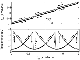
Figure 2: (a) The angle of the magnetization averaged over the soft-magnetic region $\phi_{M}$ as a function of the external field direction $\phi_{H}$. The coercivity angle $\theta_{c}$ is defined as half of the difference in $\phi_{H}$ between the paths of clock-wise and counter-clock-wise rotations of the external field, at a given $\phi_{M}$. (b) Total energy of the system. At the transition the system makes transition to another local minimum of lower energy. The sense of rotation of the external field is shown by arrows.

The variation of total energy and the angle of average magnetization of the soft-hard magnet with the external field’s angle is shown in FIG. 2. Three hysteresis transitions happen within one full rotation of external magnetic field. These hystereses correspond to the switching of the system between the three equivalent minimum energy states. The energy drop during the transition is a function of the geometrical parameters of the system and the magnitude of applied field.

The regular definition of coercive field does not apply in our case because the angle, and not the magnitude of the applied field, is varied. The same magnetic configuration can be reached either by a clockwise or by a counter-clockwise rotation of the external magnetic field. Because of the presence of hysteresis in the system, these two angles would not be the same. We define our coercive field angle, $\theta_{c}$, to be half of the difference between these two external field angles [FIG. 2(a)]. For the geometrical parameters of the system mentioned above, the coercive field angle is about $0.15$ radians for an external field of $250$ Oersteds. As the external field intensity is increased, the energy drop during transition decreases, because of the earlier onset of collapse of current configuration to another energetically favorable one. For our sample geometry, $H_{c}$, the critical field below which there are no transitions, is approximately $100$ Oersteds.

The scale of variation of magnetization on the plane of the soft magnet is characterized by only one parameter in this system: $J$, the exchange coefficient. An increase in $J$ is equivalent to increasing the length scale of magnetization and reducing the scale of sample geometry. Therefore, increasing $J$ increases the energy drop during transition from one minimum to another. This is observed in our system. Similarly, $H_{c}$ scales with $J$.

Now we discuss the application of magnetic hysteresis to moving a free magnetic nanoparticle in the device sketched in FIG. 1(a). Because of the complex magnetic dipole distribution of the soft-hard magnetic system that arises due to the interaction between hard and soft magnets, the energy experienced by a point magnetic dipole just above the soft-hard magnet due to the magnetic field created by the soft-hard magnet exhibits multiple minima on the surface. The minima are located at high magnetic field intensity positions, since the energy experienced by the mobile nanoparticle equals $-\bm{\mu}\cdot[{\bf B}(x,y,z)+{\bf H}]$, where ${\bf B}(x,y,z)$ is the magnetic field at a point $(x,y,z)$ above the soft-hard magnet created by the magnetic dipoles present in the soft-hard magnet , ${\bf H}$ is the externally applied magnetic field, and ${\bf\mu}$ is the total magnetic moment of the magnetic nanoparticle, measured in the CGS units of magnetic moments/cm³. We assume that the magnetic nanoparticle’s magnetic moment aligns with the direction of the magnetic field at its position. The nanoparticle chooses points where $|{\bf B}(x,y,z)+{\bf H}|$ is maximum. FIG. 3 shows snapshots of movement of magnetic energy minima due to the rotating external magnetic field, $z=10$ nm above the soft-hard magnet.

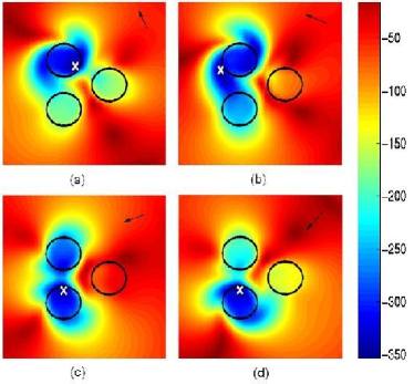
Figure 3: (a-d) This sequence of figures show the movement of magnetic energy minima as experienced by a small nanomagnet on top of the soft-hard magnet, as the external magnetic field of strength $250$ Oersteds is rotated around, counter-clockwise. Dark arrows on top right of the figures denote the direction of the externally applied magnetic field. White $\times$ mark denotes the position of the nanomagnet on the surface. The movement of the prominent minimum from the top-left to the bottom-left hard magnetic circle only is shown. The colorbar shows the energy experienced by a $125$ nm³ sized Nickel magnetic nanoparticle of magnetization $M_{0}=0.53\times 10^{3}$ magnetic moments/cm³, in units of $10^{-1}$ meV.

If a nanomagnet, of dimensions much smaller than that of the system under consideration, is allowed to move freely on the surface of the soft-hard system, it will find the nearest magnetic energy minimum and will move along with it when the magnetic dipole configuration of the underlying soft-hard magnet changes. The movement of a nanomagnet in one such prominent energy minimum, due to the rotating magnetic field, is shown in FIG. 3.

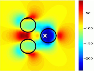
Figure 4: Magnetic energy minima as experienced by the nanomagnet on top of hard magnetic discs without the soft magnetic medium. All other conditions remain the same as that of FIG. 3.

Soft-hard magnetic surfaces are more efficient in moving nanoparticles than just hard magnetic surfaces (three discs without soft magnetic surface). This is because of the fact that magnetic energy minima can occur over soft-magnetic surface too in the former. The difference between the two can be quantified by comparing the profiles of energy minima in both these surfaces. First, the energy minima are deeper in soft-hard magnet than that of just hard magnetic surface. Typical values of energy minima would be $-35$ meV for the former, and $-25$ meV for the latter case. The higher magnetic field strength, and hence the high magnitude of energy at the minimum, is because of added soft-magnetic moments. Second, the curvature of the minima is more pronounced in soft-hard magnets. Typical values are around $0.2$ meV/nm² for the soft-hard magnetic surface, and $0.08$ meV/nm² for hard magnetic surface. This pronounced curvature traps the nanoparticle better, and gives us more control on the position of the nanoparticle. Finally, the size of the potential barrier that separates two adjacent minima is also more pronounced in soft-hard magnetic surface compared to hard magnetic surface. FIG. 4 shows the magnetic field minima on top of hard magnetic discs without the soft magnetic medium and illustrates the above mentioned differences. This system does not show any hysteretic behavior with trapped local minima. It has to be noted that the range of energies, as shown by the colorbar in FIG. 4 is narrower than the corresponding range in FIG. 3.

Because of the small size of the nanoparticle, thermal fluctuations play a role in determining the position of the nanoparticle, particularly when the multiple minima are separated by barriers of heights of the order of thermal energy. Our model includes the effects of thermal fluctuations on the nanoparticle. Area enclosed by a contour of energy $k_{B}T$ over and above the energy at the current position of the nanoparticle is accessible to the nanoparticle. The particle’s position would be the deepest minimum within the area of the contour. The schematic path of the nanoparticle during the full rotation of external magnetic field by $2{\pi}$ radians, is shown in FIG. 5. The orbit of the nanoparticle is closed.

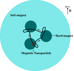
Figure 5: Schematic diagram of the path of a magnetic nanoparticle on top of soft-hard magnet. The nanoparticle traces a path similar to this when externally applied magnetic field, in the plane of soft-hard magnet, is rotated around the soft-hard magnet. The arrows show the direction of movement of the nanoparticle, when external magnetic field is rotated counter-clockwise.

We have investigated a soft-hard magnetic system with a novel planar geometry and its transitions between frustrated local energy minima. Interplay between geometrical constraints imposed by hard magnets and the exchange coupling inside soft magnet results in the display of complex magnetic patterns. We present that this rich magnetic structure can be utilized in local control of magnetization which in turn enables manipulation of position of magnetic particles. A promising direction for future work is to use an array of hard magnetic discs with their magnetizations pinned to introduce frustration, thereby creating magnetic configurations with periodicity larger than that of the unit cell of the array.

We thank Hao Zeng for helpful discussions. This work has been supported by National Science Foundation DMR-0426826.

References

- (1) R. Moessner, Can. J. Phys 79, 1283 (2001).
- (2) R. F. Wang, C. Nisoli, R. S. Freitas, J. Li, W. McConville, B. J. Cooley, M. S. Lund, N. Samarth, C. Leighton, V. H. Crespi, P. Schiffer, Nature 439, 303 (2006).
- (3) E. F. Kneller and R. Hawig, IEEE Trans. Magn 27, 3588 (1991).
- (4) R. Coehoom, D. B. de Mooji, J. P. B. Duchateau, and K. H. J. Buschow, J. Phys. Colloq 49, C8-669 (1988).
- (5) H. Zeng, J. Li, J. P. Liu, Z. L. Wang, S. Sun, Nature 420, 395 (2002).
- (6) Eiichi Goto, Nobuo Hayashi, Takaaki Miyashita and Keisuke Nakagawa, J. Appl. Phys 36, No. 9, 2951 (1965).
- (7) R. F. Sabiryanov and S. S. Jaswal, Phys. Rev. B 58, 12071 (1998).
- (8) R. F. Sabiryanov and S. S. Jaswal, J. Magn. Magn. Mater. 177 181, 989 (1998).
- (9) Giovanni Asti, Massimo Solzi, Massimo Ghidini, and Franco M. Neri, Phys. Rev. B 69, 174401 (2004).
- (10) H. C. Siegmann, J. Phys.: Condens. Matter 4, No. 44, 8395 (1992).
- (11) R. Rohlsberger, H. Thomas, K. Schlage, E. Burkel, O. Leupold, and R. Ruffer, Phys. Rev. Lett 89, 237201 (2002).
- (12) O. Hellwig, J. B. Kortright, K. Takano, and E. E. Fullerton, Phys. Rev. B 62, 11694 (2000).
- (13) C. Stamm, F. Marty, A. Vaterlaus, V. Weich, S. Egger, U. Maier, U. Ramsperger, H. Fuhrmann, and D. Pescia, Science 282, 449 (1998).
- (14) C. Gosse and V. Croquette, Biophys. J 82(6), 3314 (2002).
- (15) A. H. B. de Vries, B. E. Krenn, R. van Driel, J. S. Kanger, Biophys. J 88, 2137-2144 (2005).
- (16) J. Yan, D. Skoko, and J. F. Marko, Phys. Rev. E 70, 011905 (2004).
- (17) X. Trepat, M. Grabulosa, L. Buscemi, F. Rico, B. Fabry, J. J. Fredberg and R. Farr , Rev. Sci. Instrum 74, 4012 (2003).
- (18) E. Mirowski, J. Moreland, S. E. Russek, and M. J. Donahue, Appl. Phys. Lett 84, 1786 (2004).
- (19) J. E. Han and Vincent H. Crespi, Phy. Rev. Lett 89, 197203 (2002).
- (20) Charles Kittel, Rev. Mod. Phys 21, 541 (1949).
- (21) M. C. Payne, M. P. Teter, D. C. Allan, T. A. Arias, and J. D. Joannopoulos, Rev. Mod. Phys 64, 1045 (1992).
- (22) W. H. Press et al., Numerical Recipes in C (Cambridge University Press, Cambridge, England, 1992)