Discrete Nonlinear Breathing Modes in Carbon Nanotubes

Abstract

We study large-amplitude oscillations of carbon nanotubes with chiralities $(m,0)$ and $(m,m)$ and predict the existence of localized nonlinear modes in the form of discrete breathers. In nanotubes with the index $(m,0)$ three types of localized modes can exist, namely longitudinal, radial, and twisting breathers; however only the twisting breathers, or twistons, are nonradiating nonlinear modes which exist in the frequency gaps of the linear spectrum. Geometry of carbon nanotubes with the index $(m,m)$ allows only the existence of broad radial breathers in a narrow spectral range.

Carbon nanotubes book are attracting considerable attention in recent years after their discovery by Iijima disc . They can be thought of as cylinders of carbon atoms arranged in hexagonal grids and are thus fullerene-related structures. The growing interest to study carbon nanotubes can be explained by their unique physical properties and their potential for a wide range of possible applications. In particular, the carbon nanotubes are known for their superior mechanical strength ref_1 and good heat conductance ref_2 . In addition, it is well established that C₆₀ fullerenes can support large-amplitude oscillations rao which can be excited and controlled by temporally shaped laser pulses laa_prl .

In the continuum approximation, nonlinear dynamics of carbon nanotubes has been analyzed by several groups and, in particular, supersonic longitudinal compression solitons described by the effective Korteweg-de Vries equation have been predicted to exist in such structures, similar to other simpler discrete lattices ast_prb . However, the recent numerical modeling of more complete discrete model of carbon nanotubes has demonstrated savin that acoustic solitons do not exist in such curved structures, and their supersonic motion is always accompanied by strong radiation of phonons.

In this Letter, we focus on the study of large-amplitude oscillating modes of carbon nanotubes that have the additional features of being nonlinear as well as discrete. We reveal that both nonlinearity and discreteness induce localization of anharmonic oscillations and, as a result, the combination of both leads to the generation of specific spatially localized modes of the type of discrete breathers sie_tak ; mac_aub . These modes act like stable effective impurity modes that are dynamically generated and may alter dramatically many properties of carbon nanotubes.

Discrete breathers appear in strongly nonlinear systems, and their spatial size become comparable to the lattice spacing. Such discrete breathers–also called ‘intrinsic localized modes’ or ‘discrete solitons’ are responsible for energy localization in the dynamics of discrete nonlinear lattices flach ; phys_today . The manipulation of the discrete breathers has been achieved in systems as diverse as annular arrays of coupled Josephson junctions jj , optical waveguide arrays optics , and antiferromagnetic spin lattices sievers . The direct observation of highly localized, stable, nonlinear excitations at the atomic level in the structures such as carbon nanotubes will underscore their importance in physical phenomena at all scales. In this Letter we demonstrate that carbon nanotubes with the index $(m,0)$ support at least three types of discrete breathers, whereas nanotubes with the index $(m,0)$ support only one type of discrete breather.

Figure 1: Schematic of a carbon nanotube with the index $(m,0)$. Below: an effective one-dimensional diatomic chain.

The structure of a carbon nanotube is shown schematically in Fig. 1. In static, the nanotube is characterized by its radius $R$ and two step parameters $h_{1}$ and $h_{2}$. In each layer, the nanotube has $m$ atoms separated by the angular distance $\Delta\phi=2\pi/m$, so that $h_{1}$ and $h_{2}$ define alternating longitudinal distances between the transverse layers. We consider such dynamics of the nanotube that all atoms in one transverse layer have identical displacements. In this case, the carbon nanotube can be modeled by an effective one-dimensional diatomic chain, where the coordinates of atoms $(\rho_{n,l}\cos\varphi_{n,l},\leavevmode\nobreak\ \rho_{n,l}\sin\varphi_{n,l},\leavevmode\nobreak\ z_{n})$ are defined by the equations: $\rho_{n,l}=R+r_{n}(t)$; $\varphi_{n,l}=\Delta\phi(l-1)+\phi_{n}(t)$, $z_{n,l}=(2k-2)(h_{1}+h_{2})+u_{n}(t)$ for $n=4k-1$; $\varphi_{n,l}=\Delta\phi(l-1)+\Delta\phi/2+\phi_{n}(t)$, $z_{n,l}=(2k-2)(h_{1}+h_{2})+h_{1}+u_{n}(t)$ for $n=4k$; $\varphi_{n,l}=\Delta\phi(l-1)+\Delta\phi/2+\phi_{n}(t)$, $z_{n,l}=(2k-1)(h_{1}+h_{2})+u_{n}(t)$ for $n=4k+1$; and $\varphi_{n,l}=\Delta\phi(l-1)+\phi_{n}(t)$, $z_{n,l}=(2k-1)(h_{1}+h_{2})+h_{1}+u_{n}(t)$ for $n=4k+2$, where the index $n=4k+i$, $(k=0,\pm 1,\pm 2,...,\leavevmode\nobreak\ i=-1,0,1,2)$ stands for the number of the transverse atomic layer, the index $l=1,...,m$ marks an atom in the transverse layer, $r_{n}(t)$ is a relative change of the radius of the $n$-th transverse layer, $\phi_{n}$ is the angle of rotation of the atoms in the layer, and $u_{n}$ is a relative longitudinal displacement of the atoms from their equilibrium position. In the static case, $r_{n}\equiv 0$, $\phi_{n}\equiv 0$, and $u_{n}\equiv 0$.

In this case, complex three-dimensional dynamics of a nanotube can be reduced to the analysis of an effective one-dimensional model with two atoms per its unit cell, and Hamiltonian of this model can be written in the form,

$$H{=}\sum_{n}[E_{2n}{+}E_{2n+1}{+}Z({\bf y}_{2n-2};{\bf y}_{2n-1};{\bf y}_{2n};{\bf y}_{2n+1})],$$ (1)

where $E_{n}=M[\dot{r}_{n}^{2}+(R+r_{n})^{2}\dot{\phi}_{n}^{2}+\dot{u}_{n}^{2}]/2$ is the kinetic energy , $M$ is the mass of a carbon atom (the total energy of the nanotube is $mH$), and the vector ${\bf y}_{n}=(r_{n},\phi_{n},u_{n})$. The interatomic potential can be written in the form,

$$Z({\bf y}_{1},{\bf y}_{2},{\bf y}_{3},{\bf y}_{4})=V({\bf x}_{1},{\bf x}_{2})+V({\bf x}_{2},{\bf x}_{3})+V({\bf x}_{2},{\bf x}_{4})\leavevmode\nobreak\$$

$$+U({\bf x}_{2},{\bf x}_{3},{\bf x}_{5})+U({\bf x}_{6},{\bf x}_{3},{\bf x}_{2})+U({\bf x}_{6},{\bf x}_{3},{\bf x}_{5})\leavevmode\nobreak\$$

$$+U({\bf x}_{1},{\bf x}_{2},{\bf x}_{3})+U({\bf x}_{1},{\bf x}_{2},{\bf x}_{4})+U({\bf x}_{3},{\bf x}_{2},{\bf x}_{4})\leavevmode\nobreak\$$

$${+}W({\bf x}_{6},{\bf x}_{3},{\bf x}_{2},{\bf x}_{5}){+}W({\bf x}_{6},{\bf x}_{3},{\bf x}_{5},{\bf x}_{2}){+}W({\bf x}_{2},{\bf x}_{3},{\bf x}_{6},{\bf x}_{5})\leavevmode\nobreak\$$

$${+}W({\bf x}_{1},{\bf x}_{2},{\bf x}_{4},{\bf x}_{3}){+}W({\bf x}_{1},{\bf x}_{2},{\bf x}_{3},{\bf x}_{4}){+}W({\bf x}_{3},{\bf x}_{2},{\bf x}_{1},{\bf x}_{4}),$$

where the coordinate vectors ${\bf x}_{i}=(x_{i},y_{i},z_{i})$, $i=1,2,...,6$ are defined as: $x_{6}=(R+r_{1})\cos(\Delta\phi+\phi_{1})$, $y_{6}=(R+r_{1})\sin(\Delta\phi+\phi_{1})$, $z_{6}=-h_{2}+u_{1}$, $x_{1}=(R+r_{2})\cos(\phi_{2})$, $y_{1}=(R+r_{2})\sin(\phi_{2})$, $z_{1}=u_{2}$, $x_{3}=(R+r_{2})\cos(\Delta\phi+\phi_{2})$, $y_{3}=(R+r_{2})\sin(\Delta\phi+\phi_{2})$, $z_{3}=u_{2}$, $x_{2}=(R+r_{3})\cos(\Delta\phi/2+\phi_{3})$, $y_{2}=(R+r_{3})\sin(\Delta\phi/2+\phi_{3})$, $z_{2}=h_{1}+u_{3}$, $x_{5}=(R+r_{3})\cos(3\Delta\phi/2+\phi_{3})$, $y_{5}=(R+r_{3})\sin(3\Delta\phi/2+\phi_{3})$, $z_{5}=h_{1}+u_{3}$, $x_{4}=(R+r_{4})\cos(\Delta\phi/2+\phi_{4})$, $y_{4}=(R+r_{4})\sin(\Delta\phi/2+\phi_{4})$, $z_{4}=h_{1}+h_{2}+u_{4}$. The potential $V({\bf x}_{1},{\bf x}_{2})=D\{\exp(-\alpha[\rho-\rho_{0}])-1\}^{2}$,  $\rho=|{\bf x}_{2}-{\bf x}_{1}|$, describes a change of the deformation energy due to interaction between two atoms with the coordinates ${\bf x}_{1}$ and ${\bf x}_{2}$. Potential $U({\bf x}_{1},{\bf x}_{2},{\bf x}_{3})=\epsilon_{v}(\cos\varphi+1/2)^{2}$, where $\cos\varphi=({\bf v}_{1},{\bf v}_{2})/(|\bf{v}_{1}|\cdot|\bf{v}_{2}|)$, and ${\bf v}_{1}={\bf x}_{2}-{\bf x}_{1}$, ${\bf v}_{2}={\bf x}_{3}-{\bf x}_{2}$, describes the deformation energy of the angle between the links ${\bf x}_{1}{\bf x}_{2}$ and ${\bf x}_{2}{\bf x}_{3}$. Finally, the potential $W({\bf x}_{1},{\bf x}_{2},{\bf x}_{3},{\bf x}_{4})=\epsilon_{t}(1-\cos\phi)$, where $\cos\phi=(\bf{u}_{1},\bf{u}_{2})/(|\bf{u}_{1}|\cdot|\bf{u}_{2}|)$ and $\bf{u}_{1}=({\bf x}_{2}-{\bf x}_{1})\times({\bf x}_{3}-{\bf x}_{2})$, $\bf{u}_{2}=({\bf x}_{3}-{\bf x}_{2})\times({\bf x}_{4}-{\bf x}_{3})$, describes the deformation energy associated with a change of the effective angle between the planes ${\bf x}_{1}{\bf x}_{2}{\bf x}_{3}$ and ${\bf x}_{2}{\bf x}_{3}{\bf x}_{4}$. We take the mass of carbon atom as $M=12m_{p}$, where $m_{p}$ if the proton mass, the length $\rho_{0}=1.418$Å, and energy $D=4.9632$ eV. Other model parameters such as $\alpha$, $\epsilon_{v}$, and $\epsilon_{t}$ can be determined from the phonon frequency spectrum of a plane of carbon atoms.

A flat plane of the carbon atoms (graphene) is a special case of carbon nanotubes in the limit $R\rightarrow\infty$, when $h_{1}=\rho_{0}/2$ and $h_{2}=\rho_{0}$. For such a plane the motion equation splits into the equations for longitudinal and transverse motion. The corresponding Hamiltonian takes a simpler form,

$$H=\sum_{n}[\frac{1}{2}M(\dot{u}_{2n-1}^{2}+\dot{u}_{2n}^{2})+V_{1}(\rho_{2n})+V_{2}(\rho_{2n-1})],$$ (2)

where $\rho_{n}=u_{n+1}-u_{n}$, the potentials $V_{1}(w)=D[\exp(-\alpha w)-1]^{2}$, $V_{2}(w)=2D\{\exp(-\alpha[a_{+}(w)^{1/2}-\rho_{0}])-1\}^{2}+2\epsilon_{v}[a_{-}(w)/a_{+}(w)+1/2]^{2}+4\epsilon_{v}[(w+\rho_{0}/2)/\sqrt{a_{+}(w)}-1/2]^{2}$, and function $a_{\pm}(w)=(w+\rho_{0}/2)^{2}\pm 3\rho_{0}^{2}/4$.

The stiffness parameters of the potentials are $K_{1}=V_{1}^{\prime\prime}(0)=2D\alpha^{2}$ and $K_{2}=V_{2}^{\prime\prime}(0)=D\alpha^{2}+27\epsilon_{v}/2\rho_{0}^{2}$. After linearizing the equation of motion following from the Hamiltonian (2), we obtain the dispersion relation for longitudinal phonons, $\omega_{\pm}(q)=\{(K_{1}+K_{2}\pm[(K_{1}+K_{2})^{2}-2K_{1}K_{2}(1-\cos 2q)]^{1/2})/M\}^{1/2}$, which are depicted in Fig. 2. The frequency spectrum consists of the acoustic $[\omega_{-}(0),\omega_{-}(\pi/2)]$ and optical $[\omega_{+}(\pi/2),\omega_{+}(0)]$ bands where $\omega_{-}(0)=0$,   $\omega_{+}(0)=\sqrt{2(K_{1}+K_{2})/M}$,   $\omega_{-}(\pi/2)=\sqrt{2K_{2}/M}$, and   $\omega_{+}(\pi/2)=\sqrt{2K_{1}/M}$.

The edge frequencies of the optical band can be estimated from the experimental data: $\omega_{+}(\pi/2)\approx 1200$ cm^-1 and $\omega_{+}(0)\approx 1600$ cm^-1 p1 . These values allow us to determine the stiffness parameters, $K_{1}=508.98$ N/m and $K_{2}=395.87$ N/m, and find the maximum frequency of acoustic phonons, $\omega_{-}(\pi/2)=1058.3$ cm^-1. Knowing the values of $K_{1}$ and $K_{2}$, we then find other parameters, $\alpha=1.7889$ Å^-1 and $\epsilon_{v}=1.3143$ eV. The value of the torsion potential $\epsilon_{t}$ can be evaluated from the maximum frequency of the transverse oscillations of a plane carbon lattice. For $\epsilon_{t}=0.2$ eV, we find the value 570 cm^-1. In order to find the parameters $R$, $h_{1}$, and $h_{2}$, we should solve the minimum problem $Z({\bf 0},{\bf 0},{\bf 0},{\bf 0})\rightarrow\min_{R,h_{1},h_{2}}$. The resulting value of energy is then used as the minimum value.

A simple form of the Hamiltonian (2) allows to obtain analytical results for the nonlinear dynamics similar to the case of diatomic lattices. These results allow to predict the existence of discrete breathers with the frequencies below the lowest optical frequency of the longitudinal phonons [see Fig. 2(c)]. The form of this breather is shown in Fig. 3. The breather is characterized by the frequency $\omega$, energy $E$, width of the localization region, $L$, and the chain extension $A$. The breather frequency is inside the band [1162, 1200] cm^-1 near the lowest edge of the longitudinal optical oscillations. For decreasing $\omega$, both $E$ and $A$ grow monotonically, and the breather width decreases.

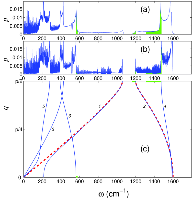
Figure 2: Spectral density of thermal oscillations of a carbon nanotube $(10,0)$ for the temperature (a) $T=300$K and (b) $T=30$K. (c) Dispersion curves of the phonons: acoustic (1) and optical (2) longitudinal phonons, acoustic (3) and optical (4) rotation phonons, and acoustic (5) and optical (6) radial phonons. For comparison, red dashed lines show the dispersion curves of longitudinal oscillations of a plane of carbon. Green color marks the frequency spectrum of breathers.

Hamiltonian (1) defines the motion equations of the system. We have studied these equations numerically and revealed that they support the existence of three types of strongly localized nonlinear modes–discrete breathers. The first type, longitudinal breathers, also exists in planar carbon structures, such breathers exist in the frequency range [1162, 1200] cm^-1. The second type, radial breathers, describes transverse localized nonlinear modes with the frequency band [562, 580] cm^-1. The third type, twisting breathers, characterizes localization of the torsion oscillations of the nanotube with the frequencies [1310, 1477] cm^-1. The frequency spectra of the breathers are shown in Fig. 2.

For a flat plane of carbon atoms, the longitudinal breathers are nonlinear modes [see Figs. 3(a,c)], and they are exact solutions of the nonlinear motion equations. However, in the case of a curved geometry, the longitudinal breathers become coupled to transverse linear modes, and they always emit some radiation. This radiation is defined by the curvature of the nanotube and its index $m$. Therefore, the longitudinal breathers are not genuine nonlinear modes of carbon nanotubes, and they possess a finite lifetime which however may exceed a few hundred of picoseconds.

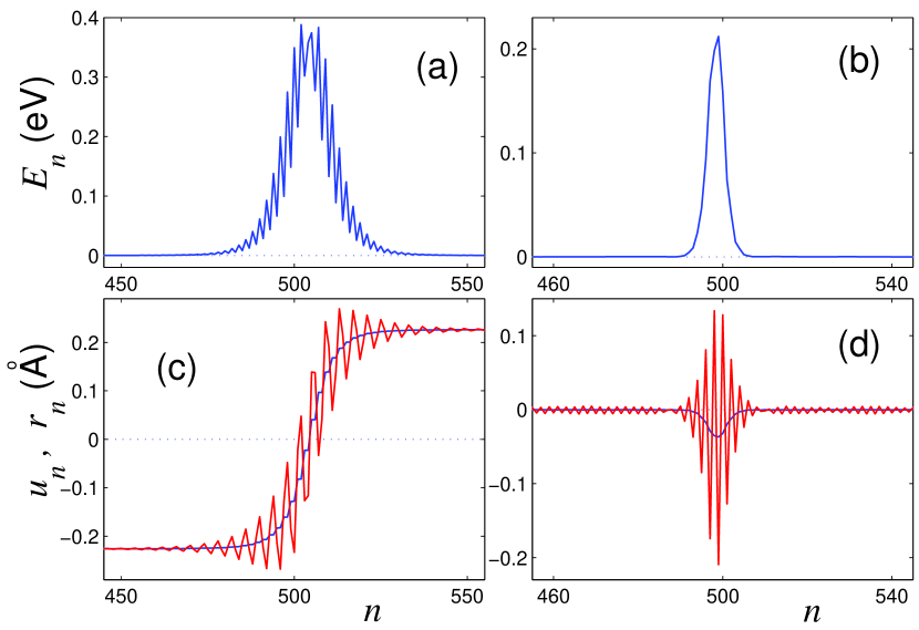
Figure 3: Example of a localized nonlinear mode of the longitudinal oscillations described by the Hamiltonian (2) (a), (b) (frequency $\omega=1164$cm^-1, energy $E=5.71$eV, width $L=16.3$, the chain extension $A=0.45$Å) and example of a radial breather (c), (d) describing localized transverse oscillations of a nanotube (10,0) with the frequency $\omega=579.6$ cm^-1, energy $E=0.99853$eV, and width $L=32.7$. Shown are (a) and (c) the averaged (in time) energy distribution $E_{n}$ in the chain, (b) the atom displacements $u_{n}$, and (d) transverse displacements $r_{n}$. In sections (b) and (d) blue lines show the values averaged over the period, red – maximal displacements. Radiation of longitudinal waves by a radial breather is clearly visible in section (d).

The second type of discrete breathers we found is associated with the localization of transverse radial oscillations of a nanotube. Example of this radial breather in the nanotube (10,0) is shown in Figs. 3(b,d). Localized out-phase transverse oscillations of the neighboring atoms lead to localized contraction and extension of the nanotube. Such transverse oscillations become coupled to the longitudinal oscillations and, therefore, the radial breathers radiate longitudinal phonons. As a result, the radial breathers are also not genuine nonlinear localized modes of the carbon nanotubes, and they decay slow by emitting small-amplitude phonons. The lifetime of these breathers can be of the order of several nanoseconds.

The third type of localized mode is a twisting breather, or twiston, associated with the torsion oscillations of the nanotube. In a sharp contrast to other two breathing modes, the twisting breather is an exact solution of the motion equations of the nanotube, and it does not radiate phonons. An example of this genuine discrete breather is shown in Fig. 4. In the localized region of this mode, the nanotube is expanded transversally being contracted longitudinally. The twiston has a broad frequency spectrum, and its energy, amplitude of the transverse extension (see Fig. 5), and the amplitude of torsion oscillations all grow with the frequency. The breather width changes monotonically, and for the frequencies $\omega<1450$ cm^-1 it becomes comparable with the lattice spacing, so that the breather becomes a highly localized mode.

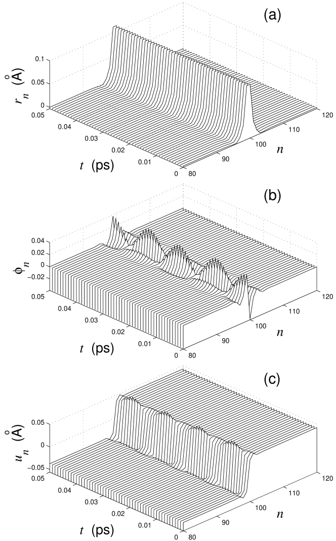
Figure 4: Dependence of (a) transverse $r_{n}$, (b) torsion $\phi_{n}$, and (c) longitudinal $u_{n}$ displacements of the twisting discrete breather (frequency $\omega=1367$ cm^-1, energy $E=1.6465$ eV, width $L=1.55$) on the time $t$.

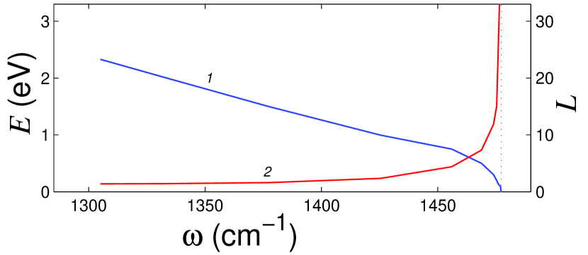
Figure 5: Dependence of total energy $E$ (curve 1) and width $L$ (curve 2) of the twisting discrete breather on the frequency $\omega$. Vertical line show the edge of the linear spectrum of optical torsion oscillations in the (10,0) nanotube.

Next, we analyze thermal oscillations of a carbon nanotube by employing the Langevin equations. We find that for low temperatures ($T=30$K) the oscillations are mostly linear and the frequency density does not differ much from the density of linear modes, as demonstrated in Fig. 2(b). However, for higher temperatures ($T=300$K) the spectral density acquires specific features associated with the generation of nonlinear modes, as can be seen in Fig. 2(a) where we observe thermal oscillations with the frequencies inside the linear spectral gaps which can be associated with discrete breathers. Indeed, the larger contribution of these nonlinear modes is for the torsion oscillations of the twisting breathers, which are stable and have the largest frequency spectrum.

We have carried out the similar nonlinear analysis for the nanotubes with the index $(m,m)$ and revealed that in this nanotube can support only one type of breathers, a radial breather with a very narrow frequency spectrum [430.5, 436] cm^-1 near the upper edge of the frequency band of radial phonons. However, this radial breather is not an exact solution of the nonlinear motion equations, and radiation of small-amplitude linear waves leads to a decay of the breather. As a result, the existence of nonlinear localized modes depends crucially on chirality of the carbon nanotube, so that genuine discrete breathers are expected to exist in the nanotube with the index $(m,0)$. Existence of twisting breathers is due to the anharmonic interaction potential, and the large spectral gap in the frequency spectrum of torsion phonons. However, the radial long-lived nonlinear modes can appear in the nanotubes with any type of chirality.

In conclusion, we have revealed that carbon nanotubes can support spatially localized large-amplitude stable nonlinear modes in the form of discrete breathers, and we have analyzed the existence and stability of three types of breathers. A novel type of such highly localized discrete modes –twistons– is associated with the energy self-trapping of torsion oscillations of the carbon nanotubes.

This work was supported by the Australian Research Council. Alex Savin thanks the Nonlinear Physics Center of the Australian National University for a warm hospitality during his stay in Canberra.

References

- (1) R. Saito, G. Dresselhaus and M.S. Dresselhaus, Physical Properties of Carbon Nanotubes (Imperial College Press, London, 1998).
- (2) S. Iijima, Nature (London) 354, 56 (1991).
- (3) M.M.J. Treacy, T.W. Ebbesen, and J.M. Gibson, Nature (London) 381, 678 (1996).
- (4) S. Berber et al., Phys. Rev. Lett. 84, 4613 (2000).
- (5) A. Rao et al., Science 275, 187 (1997).
- (6) T. Laarmann et al., Phys. Rev. Lett. 98, 058302 (2007).
- (7) T.Yu. Astakhova et al., Phys. Rev. B 64, 035418 (2001).
- (8) A.V. Savin and O.I. Savina, Phys. Solid State 46, 383 (2004).
- (9) A.J. Sievers and S. Takeno, Phys. Rev. Lett. 61, 970 (1988).
- (10) R.S. MacKay and S. Aubry, Nonlinearity 7, 1623 (1994).
- (11) S. Flach and C.R. Willis, Phys. Rep. 295, 182 (1998).
- (12) D.K. Campbell, S. Flach, and Yu.S. Kivshar, Phys. Today 57, 43 (2004).
- (13) E. Trías et al., Phys. Rev. Lett. 84, 741 (2000); P. Binder et al., Phys. Rev. Lett. 84, 745 (2000).
- (14) H.S. Eisenberg et al., Phys. Rev. Lett. 81, 3383 (1998).
- (15) M. Sato and A.J. Sievers, Nature 432, 486 (2004).
- (16) R. Al-Jishi and G. Dresselhaus, Phys. Rev. B 26, 4514 (1982).