Dynamics of domain walls in magnetic nanostrips

Abstract

We express dynamics of domain walls in ferromagnetic nanowires in terms of collective coordinates generalizing Thiele’s steady-state results. For weak external perturbations the dynamics is dominated by a few soft modes. The general approach is illustrated on the example of a vortex wall relevant to recent experiments with flat nanowires. A two-mode approximation gives a quantitatively accurate description of both the steady viscous motion of the wall in weak magnetic fields and its oscillatory behavior in moderately high fields above the Walker breakdown.

Dynamics of domain walls in nanosized magnetic wires, strips, rings etc. is a subject of practical importance and fundamental interest Atkinson et al. (2003); Thiaville and Nakatani (2006). Nanomagnets typically have two ground states related to each other by the symmetry of time reversal and thus can serve as a memory bit. Switching between these states proceeds via creation, propagation, and annihilation of domain walls with nontrivial internal structure and dynamics. Although domain-wall (DW) motion in macroscopic magnets has been studied for a long time Hubert and Schäfer (1998), new phenomena arise on the submicron scale where the local (exchange) and long-range (dipolar) forces are of comparable strengths DeSimone et al. (2006). In this regime, domain walls are textures with a rich internal structure McMichael and Donahue (1997); Thiaville and Nakatani (2006). As a result, they have easily excitable internal degrees of freedom. Providing a description of the domain-wall motion in a nanostrip under an applied magnetic field is the main subject of this paper. We specialize to the experimentally relevant case of thin strips with a thickness-to-width ratio $t/w\ll 1$.

The dynamics of magnetization is described by the Landau-Lifshitz-Gilbert (LLG) equation Landau and Lifshitz (1935)

$$\dot{\mathbf{m}}=\gamma\mathbf{H}_{\mathrm{eff}}\times\mathbf{m}+\alpha\,\mathbf{m}\times\dot{\mathbf{m}}.$$ (1)

Here $\mathbf{m}=\mathbf{M}/|\mathbf{M}|$, $\mathbf{H}_{\mathrm{eff}}(\mathbf{r})=-\delta U/\delta\mathbf{M}(\mathbf{r})$ is an effective magnetic field derived from the free-energy functional $U[\mathbf{M(r)}]$, $\gamma=g|e|/2mc$ is the gyromagnetic ratio, and $\alpha\ll 1$ is Gilbert’s damping constant Gilbert (2004). Equation (1) can be solved exactly only in a few simple cases. Walker Schryer and Walker (1974) considered a one-dimensional domain wall $\mathbf{m}=\mathbf{m}(x,t)$ in a uniform external magnetic field ${\mathbf{H}}||x$. At a low applied field the wall exhibits steady motion, $\mathbf{m}=\mathbf{m}(x-vt)$, with the velocity $v\approx\gamma H\Delta/\alpha$, where $\Delta$ is the wall width. Above a critical field $H_{W}=\alpha M/2$ magnetization starts to precess, the wall motion acquires an oscillatory component and the average speed of the wall drops sharply. Qualitatively similar behavior has been observed in magnetic nanostrips Atkinson et al. (2003), however, numerical studies demonstrate that Walker’s theory fails to provide a quantitative account of both the steady and oscillatory regimes Thiaville and Nakatani (2006).

We formulate the dynamics of a magnetic texture in terms of collective coordinates $\bm{\xi}(t)=\{\xi_{0},\xi_{1},\ldots\}$, so that $\mathbf{m}(\mathbf{r},t)={\mathbf{m}}(\mathbf{r},\{\bm{\xi}(t)\})$. Although a magnetization field has infinitely many modes, its long-time dynamics—most relevant to the motion of domain walls—is dominated by a small subset of soft modes with long relaxation times. Focusing on soft modes and ignoring hard ones reduces complex field equations of magnetization dynamics to a much simpler problem. In Walker’s problem, the soft modes are the location of the domain wall and the precession angle; the width of the wall is a hard mode Thiaville and Nakatani (2006); Schryer and Walker (1974). Partition of modes into soft and hard depends on characteristic time scales, determined e.g. by the strength of the driving field.

Equations of motion for generalized coordinates $\{\bm{\xi}(t)\}$ describing a magnetic texture can be derived directly from the LLG equation (1). They read

$$G_{ij}\dot{\xi}_{j}+F_{i}-\Gamma_{ij}\dot{\xi}_{j}=0.$$ (2)

Here $F_{i}(\bm{\xi})=-\partial U/\partial\xi_{i}$ is the generalized conservative force conjugate to $\xi_{i}$, while $\Gamma_{ij}=\Gamma_{ji}$ and $G_{ij}=-G_{ji}$ are the damping and gyrotropic tensors with matrix elements described below. The three terms in Eq. (2) can be traced directly to the three terms in the LLG equation (1).

To derive Eq. (2), take the cross product of Eq. (1) with $\mathbf{m}$ and express the time derivative of the magnetization in terms of generalized velocities, $\dot{\mathbf{m}}(\mathbf{r},\bm{\xi})=(\partial\mathbf{m}/\partial\xi_{j})\dot{\xi}_{j}$, to obtain

$$J\left(\mathbf{m}\times\frac{\partial\mathbf{m}}{\partial\xi_{j}}\right)\dot{\xi}_{j}=-\frac{\delta U}{\delta\mathbf{m}}-\alpha J\frac{\partial\mathbf{m}}{\partial\xi_{j}}\,\dot{\xi}_{j}.$$ (3)

Here $J=\mu_{0}M/\gamma$ is the density of angular momentum. Taking the scalar product with $\partial\mathbf{m}/\partial\xi_{i}$ and integrating over the volume of the magnet yields Eq. (2) with

$$F_{i}(\bm{\xi}) = -\int\delta U/\delta\mathbf{m}\cdot\partial\mathbf{m}/\partial\xi_{i}\,dV=-\partial U/\partial\xi_{i},$$

$$\Gamma_{ij}(\bm{\xi}) = \alpha J\int\partial\mathbf{m}/\partial\xi_{i}\cdot\partial\mathbf{m}/\partial\xi_{j}\,dV,$$

$$G_{ij}(\bm{\xi}) = J\int\mathbf{m}\cdot\left(\partial\mathbf{m}/\partial\xi_{i}\times\partial\mathbf{m}/\partial\xi_{j}\right)\,dV.$$ (4)

Eqs. (2) and (4) generalize Thiele’s result Thiele (1973) for steady translational motion of a texture to the case of arbitrary motion.

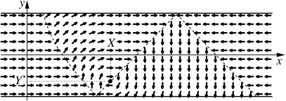
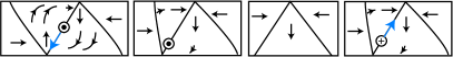
Figure 1: Top: A model of the vortex domain wall proposed in Ref. Youk et al., 2005. Dashed lines denote Neel walls emanating from the topological edge defects. Bottom: Absorption and re-emission of the vortex at the edge. Note the reversal of the polarization $p$ of the vortex core.

We apply this general approach to the dynamics of the vortex domain wall McMichael and Donahue (1997), a texture that consists of three elementary topological defects: a vortex in the bulk and two antihalfvortices confined to the edges Tchernyshyov and Chern (2005). A strong shape anisotropy forces the magnetization into the plane of the strip, with the exception of the vortex core Wachowiak et al. (2002). Soft modes of the wall are associated with the motion of these defects, and we start with a model Youk et al. (2005) parameterized by the $(X,Y)$ coordinates of the vortex (Fig. 1). In low applied fields, the wall exhibits translational motion that can be described by a single collective coordinate $\xi_{0}=X$, representing the softest (in fact, zero) mode with an infinite relaxation time $\tau_{0}=\infty$. At higher driving fields the steady motion breaks down and the vortex core exhibits oscillations in both longitudinal and transverse directions accompanied by slow drift along the strip Thiaville and Nakatani (2006). An additional dynamical variable $\xi_{1}=Y$, is required to describe the dynamics. The new mode has a finite relaxation time $\tau_{1}$. In the vortex domain wall the characteristic time of the motion is time $T$ it takes the vortex to cross the strip. When

$$\underbrace{\tau_{0}>\tau_{1}}_{\mathrm{soft}}>T>\underbrace{\tau_{2}>\tau_{3}>\ldots}_{\mathrm{hard}}\ ,$$ (5)

the soft modes $\xi_{0}$ and $\xi_{1}$ must be treated as dynamical variables. All other modes are hard; they adjust adiabatically to their equilibrium values. As the driving field increases, the vortex moves faster and eventually $T$ will become shorter than the relaxation time $\tau_{2}$ of the next mode, at which point the two-mode model will break down. While $\tau_{0}$ is infinite due to translational symmetry of the wire, $\tau_{1}$ is also long because of the special kinematics of vortex cores (see discussion below). If $\tau_{1}\gg\tau_{2}$ we expect to have a substantial range of driving fields where the two-mode approximation applies.

Next we discuss the general aspects of the dynamics in the one and two-mode regimes. We approximate the potential energy $U(X,Y)$ by its Taylor expansion to the second order in $X$ and $Y$:

$$U(X,Y)\approx-QHX-\chi rQHY+kY^{2}/2\ .$$ (6)

The $X$ dependence comes in the form of the universal Zeeman term $-QHX$, where $Q=2\mu_{0}Mtw$ is the magnetic charge of the domain wall independent of the exact shape of the texture. Zeeman force also pushes the vortex in the transverse direction, which is reflected in the linear in $Y$ term, dependent on the vortex chirality $\chi=-1(+1)$ for clockwise (counterclockwise) circulation. This term is consistent with the lack of $y\mapsto-y$ reflection symmetry; the numerical coefficient is $r\approx 2$. The transverse restoring potential $kY^{2}/2$ comes from the dipolar and exchange energies.

The antisymmetric gyrotropic tensor $G_{XY}=-G_{YX}=4\pi qJt$ reflects a special topology of the vortex core, namely its nonzero skyrmion charge Belavin and Polyakov (1975)

$$q=(1/4\pi)\int\mathbf{m}\cdot(\partial_{x}\mathbf{m}\times\partial_{y}\mathbf{m})\,d^{2}r=np/2,$$ (7)

where $n=+1$ is the O(2) winding number and $p=M_{z}/|M_{z}|=\pm 1$ is the out-of-plane polarization of the core Tretiakov and Tchernyshyov (2007). A vortex core moving at the velocity $\mathbf{V}$ experiences a gyrotropic force $\mathbf{F}^{g}=pG\,\hat{\mathbf{z}}\times\mathbf{V}$, where $G=2\pi Jt$ is the gyrotropic constant. The equations of motion (2) for two dynamic modes read

$$\left(\begin{array}[]{cc}\Gamma_{XX}&\Gamma_{XY}-pG\\ \Gamma_{XY}+pG&\Gamma_{YY}\end{array}\right)\left(\begin{array}[]{c}\dot{X}\\ \dot{Y}\end{array}\right)=\left(\begin{array}[]{c}QH\\ \chi rQH-kY\end{array}\right).$$ (8)

It is worth noting that typically $\Gamma_{ij}/G\ll 1$, which means that the viscous force is usually much weaker than the gyrotropic one Guslienko et al. (2002); Shibata et al. (2006). Therefore, a good starting point would be the frictionless limit $\Gamma_{ij}=0$. In that case the vortex moves along the lines of constant potential $U(X,Y)=\mathrm{const}$. From that one can deduce a crossing time $T=\pi/(\gamma\mu_{0}H)$ that is remarkably insensitive to the detailed structure of the domain wall Lee et al. , as indeed observed experimentally Hayashi et al. (2006). However, the viscous loss of energy is a crucial factor determining the average velocity of a domain wall: any drift reflects the dissipation of the Zeeman energy $-QHX$; in the frictionless limit the wall exhibits no drift at all. Thus one must include the effects of viscous friction to evaluate the drift velocity.

A general solution of the equations of motion (8) reads

$$X-Y(pG-\Gamma_{XY})/\Gamma_{XX}=Vt+\mathrm{const},$$ (9)

$$Y=Y_{0}e^{-t/\tau_{1}}+Y_{\infty}(1-e^{-t/\tau_{1}}),$$ (10)

where $\tau_{1}=(G^{2}+\det{\Gamma})/(k\Gamma_{XX})\approx G^{2}/(k\Gamma_{XX})$, $Y_{\infty}=-(p-\chi g)GQH/(k\Gamma_{XX})$, and $g=(r\Gamma_{XX}-\chi\Gamma_{XY})/G$. Two distinct regimes are found. At low applied field, the equilibrium position of the vortex is inside the strip. After a relaxation period of duration $\tau_{1}\sim G^{2}/(k\Gamma_{XX})$ the wall reaches a state of steady drift with $\dot{X}=V=\mu_{\mathrm{LF}}H$ ($\mu_{\mathrm{LF}}=Q/\Gamma_{XX}$ is the mobility in low fields), and $Y=Y_{\infty}\sim-p\,GV/k$. Note that in the absence of the gyrotropic force, the relaxation time would have been much shorter, $\Gamma_{YY}/k$. The gyrotropic effect is apparently one of the reasons why the mode $\xi_{1}=Y$ is particularly soft.

Above a critical field the restoring potential fails to prevent the vortex from reaching the edge, where it merges with the antihalfvortex. Our numerical experiments (see below) indicate that the vortex is immediately re-emitted with the same chirality $\chi$ and opposite polarization $p$ and starts to move towards the opposite edge (Fig. 1, bottom). The critical fields are slightly different for $p=+\chi$ and $p=-\chi$: $H_{c\pm}=H_{c0}/(1\mp g)$, where $H_{c0}=\mu_{\mathrm{LF}}kw/2G$ and $g\ll 1$. In the narrow interval $H_{c-}<H<H_{c+}$ the vortex reaches a steady state for $p=+\chi$ but not for $p=-\chi$. As one might expect, the breakdown of steady motion coincides with the softening of the first mode: at $H=H_{c0}$ the crossing time $T=2\tau_{1}$.

Above $H_{c+}$ the vortex crosses the strip regardless of its polarization, and an oscillatory regime sets in. For the drift velocity $V_{d}$ we find

$$V_{d}=\mu_{\mathrm{LF}}H-\frac{2V_{c}(1+\det{\Gamma}/G^{2})^{-1}}{\mathrm{atanh}(H_{c+}/H)+\mathrm{atanh}(H_{c-}/H)}.$$ (11)

At first, the drift velocity drops precipitously (Fig. 2), changing its order of magnitude from $\mathcal{O}(\alpha^{-1})$ to $\mathcal{O}(\alpha)$. In higher fields the velocity once again becomes proportional to $H$, albeit with a smaller mobility $\mu_{\mathrm{HF}}$:

$$\frac{\mu_{\mathrm{HF}}}{\mu_{\mathrm{LF}}}=\frac{(r^{2}\Gamma_{XX}-2r\chi\Gamma_{XY}+\Gamma_{YY})\Gamma_{XX}}{G^{2}}\ll 1.$$ (12)

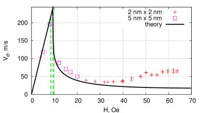
Figure 2: The drift velocity $V_{d}$ of the domain wall as a function of the applied field $H$ for a permalloy strip of width $w=200$ nm and thickness $t=20$ nm. Dashed vertical lines mark the critical fields $H_{c-}$ and $H_{c+}$. Symbols are results of numerical simulations with in-plane mesh sizes as shown.

For a quantitative analysis lon we turn to the model of a vortex domain wall of Youk et al. Youk et al. (2005). The composite wall consists of three $90^{\circ}$ Neel walls comprising the antihalfvortices and a vortex that can slide along the central Neel wall (Fig. 1). We used saturation magnetization $M=8.6\times 10^{5}\ \mathrm{A\ m^{-1}}$, Gilbert damping $\alpha=10^{-2}$, and exchange constant $A=1.3\times 10^{-11}\ \mathrm{J\ m^{-1}}$, yielding the exchange length $\lambda=\sqrt{A/\mu_{0}M^{2}}=3.8$ nm.

The damping coefficients $\Gamma_{ij}$ (4) are determined mostly by areas with a large magnetization gradient $\nabla\mathbf{m}$, i.e. from the three Neel walls whose width is of order the exchange length $\lambda$, which gives $\Gamma_{ij}\sim\alpha Jtw/\lambda$. The values of damping coefficients are as follows lon :

$$\Gamma_{XX}=0.044G,\ \Gamma_{XY}=0.031\chi G,\ \Gamma_{YY}=0.049G.$$ (13)

The stiffness constant $k$ of the restoring potential could not be calculated accurately because two of its main contributions, a positive magnetostatic term and a negative term due to Neel-wall tension, nearly cancel out. This is not surprising given the proximity to a region where the vortex wall is unstable McMichael and Donahue (1997). Instead, we extracted the relaxation time $\tau_{1}$ directly from the numerics (see below) by fitting $Y(t)$ to Eq. (10). We obtained $\tau_{1}$ in the range from 8.5 to 9 ns for fields from 4 to 60 Oe with $Y_{\infty}$ scaling linearly with $H$. In calculating the critical velocity $V_{c}=kw/(2G)$, we replaced $w$ with an effective strip width $w_{\mathrm{eff}}=w-2R$, where $R$ is a short-range cutoff due to the finite size of a vortex core Wachowiak et al. (2002). From vortex trajectories observed numerically (top panel of Fig. 3) we estimate $R\approx 10$ nm.

To compare our theory with experimental results, we have computed the low and high-field mobilities using standard material parameters for permalloy (see methods) for a strip of $w=600$ nm and $t=20$ nm employed in the experiment of Beach et al. Beach et al. (2005). While the calculated low-field mobility $\mu_{\mathrm{LF}}^{\mathrm{th}}=29\ \mathrm{m\ s^{-1}Oe^{-1}}$ agrees reasonably well with the experimental result $\mu_{\mathrm{LF}}^{\mathrm{exp}}=25\ \mathrm{m\ s^{-1}Oe^{-1}}$, our estimate of the high-field mobility $\mu_{\mathrm{HF}}^{\mathrm{th}}=0.61\ \mathrm{m\ s^{-1}Oe^{-1}}$ is markedly lower than the observed value $\mu_{\mathrm{HF}}^{\mathrm{exp}}=2.5\ \mathrm{m\ s^{-1}Oe^{-1}}$.

To understand the discrepancy between theory and experiment at high fields, we compared the theoretical curve $V_{d}(H)$ against numerically simulated motion of a vortex domain wall in a permalloy strip with width $w=200$ nm and thickness $t=20$ nm. Numerical simulations were performed using the package oommf Donahue and Porter (1999). We used the same material parameters as mentioned above. Cell sizes were $2\ \mathrm{nm}\times 2\ \mathrm{nm}\times 20\ \mathrm{nm}$ for most runs and $5\ \mathrm{nm}\times 5\ \mathrm{nm}\times 20\ \mathrm{nm}$ in a few others. The strip length was $L=4$ $\mu$m or more. Care was taken to minimize the influence of a stray magnetic field created by magnetic charges at the ends of the strip.

The drift velocity $V_{d}$ computed within the two-mode approximation agrees reasonably well with simulation results both below and above the breakdown field $H_{c+}=9.5$ Oe up to a field of $H_{2}\approx 35$ Oe (Fig. 2). However, above $H_{2}$ the numerically observed drift velocity begins to increase in disagreement with the theory. The failure of the two-mode approximation around $H_{2}$ was traced to the softening of another mode seen as fast oscillations of the width of the domain wall (the width was measured as the difference in $x$-coordinates of the antihalfvortices, top panel in Fig. 3). The new mode is excited at the beginning of each cycle and relaxes to an equilibrium on the time scale $\tau_{2}\approx 2.5$ ns. In a field of $H=24$ Oe this mode decays well before the end of the cycle ($T=7.4$ ns, see the bottom panel of Fig. 2). It is responsible for a small fraction, $\mathcal{O}(\tau_{2}/T)$, of the net energy loss and thus can be neglected. At $H=48$ Oe ($T=3.7$ ns) the new mode stays active all the time and therefore cannot be ignored. In accordance with this, the numerical data begin to deviate from our two-mode model (11) around $H_{2}=35$ Oe. The new mode is related to the incipient emission of an antivortex by one of the edge defects. A similar mechanism may be at work in wider strips used by Beach et al. Beach et al. (2005).

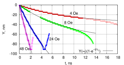
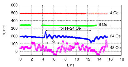
Figure 3: Top: The transverse vortex coordinate $Y(t)$ for several values of the applied field $H$. Deviations from the expected behavior (10) in weak fields are due to stray field from the strip ends. Bottom: The width of the wall $\Delta(t)$. Curves for different fields are shifted vertically by 150 nm for clarity. The initial width in all cases was $\Delta(0)=190$ nm.

The framework presented here is sufficiently simple and flexible to include additional modes and the effects of spin torque. It can also handle other scenarios observed in numerical simulations wherein the absorbed vortex is re-emitted with the opposite chirality Lee et al. or not re-emitted at all Thiaville and Nakatani (2006) or the vortex core flips while the vortex is still in the bulk Van Waeyenberge et al. (2006); Tretiakov and Tchernyshyov (2007). Antivortex walls Thiaville and Nakatani (2006); Kunz (2006); Lee et al. can be handled in a similar way, provided one develops a similarly detailed model to compute the energy and damping coefficients.

The authors thank G. S. D. Beach, C.-L. Chien, K. Yu. Guslienko, S. Komineas, A. Kunz, and F. Q. Zhu for helpful discussions and M. O. Robbins for sharing computational resources. This work was supported in part by NSF Grant No. DMR-0520491, by the JHU Theoretical Interdisciplinary Physics and Astronomy Center, and by the Dutch Science Foundation NWO/FOM.

References

- Atkinson et al. (2003) D. Atkinson et al., Nature Mat. 2, 85 (2003).
- Thiaville and Nakatani (2006) A. Thiaville and Y. Nakatani, in Spin Dynamics in Confined Magnetic Structures III (Springer, 2006).
- Hubert and Schäfer (1998) A. Hubert and R. Schäfer, Magnetic Domains (Springer, Berlin, 1998).
- DeSimone et al. (2006) A. DeSimone, R. V. Kohn, S. Mueller, and F. Otto, in The Science of Hysteresis, edited by G. Bertotti and I. Mayergoyz (Elsevier, 2006), vol. 2, chap. 4.
- McMichael and Donahue (1997) R. D. McMichael and M. J. Donahue, IEEE Trans. Magn. 33, 4167 (1997).
- Landau and Lifshitz (1935) L. D. Landau and E. M. Lifshitz, Phys. Z. Sowjetunion 8, 53 (1935).
- Gilbert (2004) T. L. Gilbert, IEEE Trans. Mag. 40, 3443 (2004).
- Schryer and Walker (1974) N. L. Schryer and L. R. Walker, J. Appl. Phys. 45, 5406 (1974).
- Thiele (1973) A. A. Thiele, Phys. Rev. Lett. 30, 230 (1973).
- Youk et al. (2005) H. Youk et al., J. Appl. Phys. 99, 08B101 (2005).
- Tchernyshyov and Chern (2005) O. Tchernyshyov and G.-W. Chern, Phys. Rev. Lett. 95, 197204 (2005).
- Wachowiak et al. (2002) A. Wachowiak et al., Science 298, 577 (2002).
- Belavin and Polyakov (1975) A. A. Belavin and A. M. Polyakov, Pis’ma ZheETF 22, 245 (1975), [JETP Lett. 22, 245 (1975)].
- Tretiakov and Tchernyshyov (2007) O. A. Tretiakov and O. Tchernyshyov, Phys. Rev. B 75, 012408 (2007).
- Guslienko et al. (2002) K. Y. Guslienko et al., J. Appl. Phys. 91, 8037 (2002).
- Shibata et al. (2006) J. Shibata et al., Phys. Rev. B 73, 020403 (2006).
- (17) J.-Y. Lee et al., eprint arXiv.org:0706.2542v1.
- Hayashi et al. (2006) M. Hayashi et al., Nat. Phys. 3, 21 (2006).
- (19) D. Clarke et al. (unpublished).
- Beach et al. (2005) G. S. D. Beach et al., Nature Mat. 4, 741 (2005).
- Donahue and Porter (1999) M. J. Donahue and D. G. Porter, Tech. Rep. NISTIR 6376, National Institute of Standards and Technology, Gaithersburg, MD (1999), http://math.nist.gov/oommf.
- Van Waeyenberge et al. (2006) B. Van Waeyenberge et al., Nature (London) 444, 461 (2006).
- Kunz (2006) A. Kunz, IEEE Trans. Mag. 42, 3219 (2006).